1 Stochastic Dynamic Optimization of Forest Industry Company Management INFORMS International...
98
1 Stochastic Dynamic Optimization of Forest Industry Company Management INFORMS International Meeting 2007 Puerto Rico Peter Lohmander Professor SLU Umea, SE-901 83, Sweden, http:// www.Lohmander.com Version 2007-06-21
-
Upload
elvis-atherley -
Category
Documents
-
view
215 -
download
0
Transcript of 1 Stochastic Dynamic Optimization of Forest Industry Company Management INFORMS International...

1
Stochastic Dynamic Optimization of Forest Industry Company Management
INFORMS International Meeting 2007 Puerto Rico
Peter LohmanderProfessor
SLU Umea, SE-901 83, Sweden, http://www.Lohmander.com
Version 2007-06-21

2
Abstract
• Forest industry production, capacity and harvest levels are optimized.
• Adaptive full system optimization is necessary for consistent results.
• The stochastic dynamic programming problem of a complete forest industry company is solved. The raw material stock level and the main product prices are state variables. In each state and at each stage, a linear programming profit maximization problem of the forest company is solved. Parameters from the Swedish forest industry are used as illustration.

3
Question
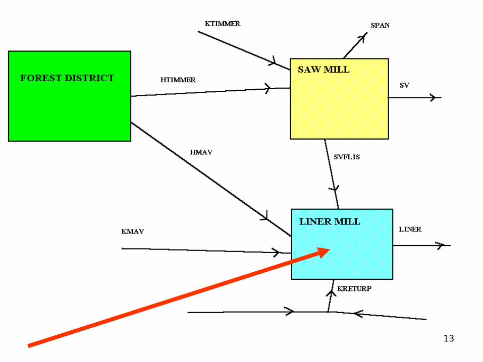
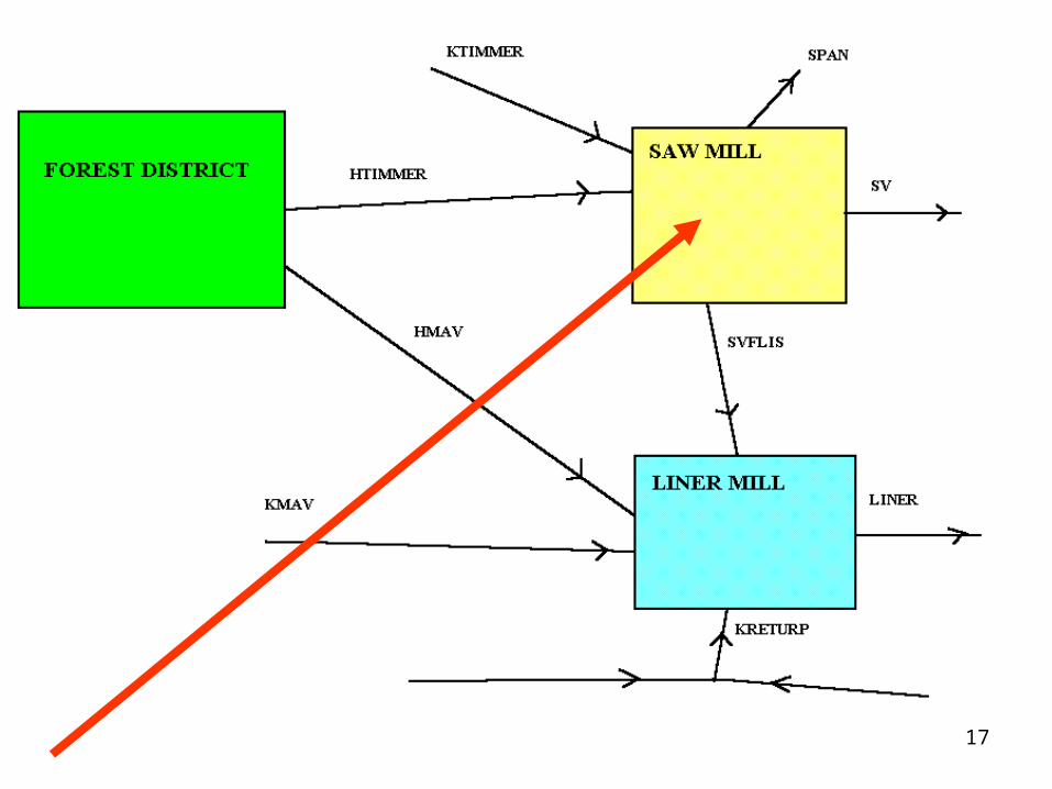
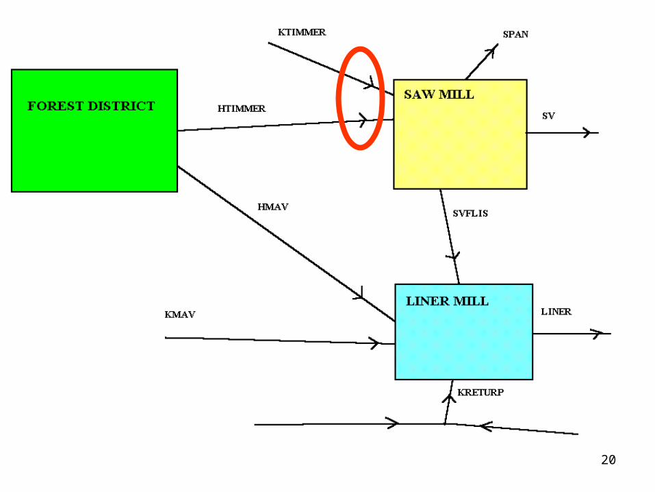
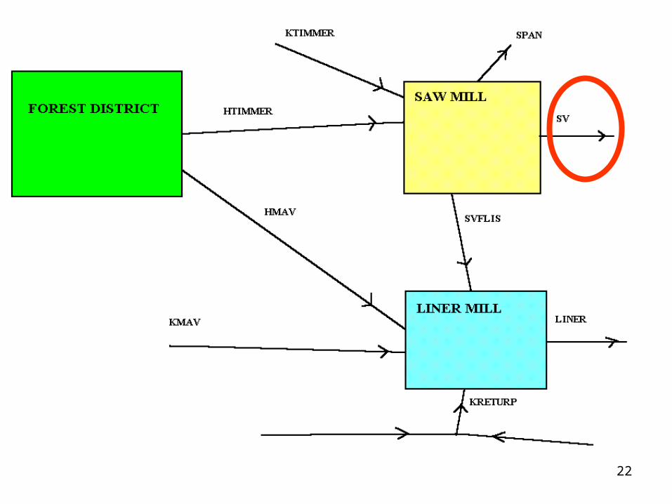
How should these activities in a typical forest industry company be optimized and coordinated in the presence of stochastic markets?
*Pulp, paper and liner production and sales,
*Sawn wood production and sales,
*Raw material procurement and sales,
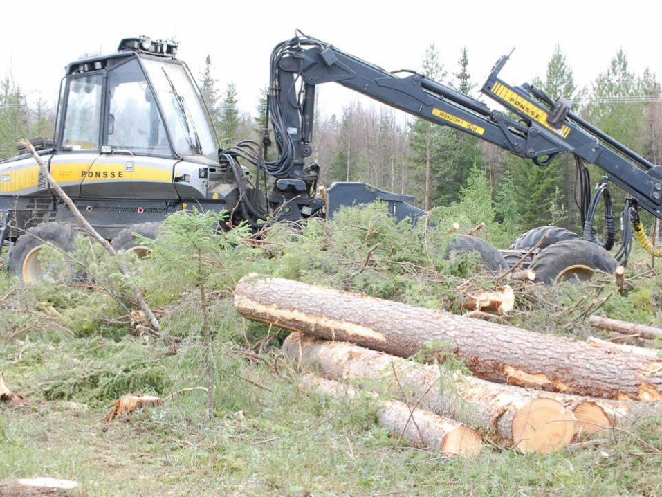
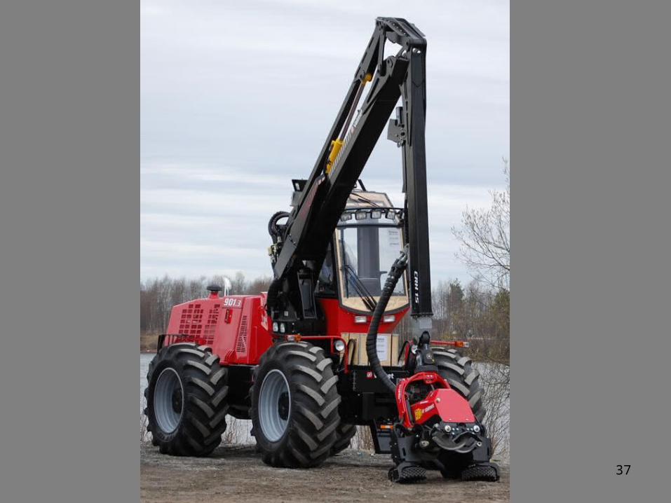
*Harvest operations
*Transport
4
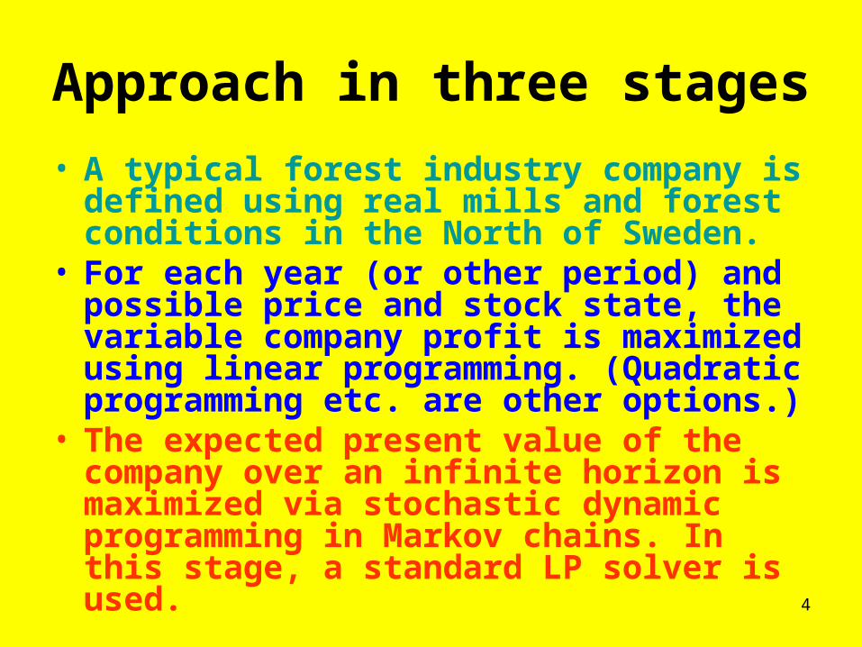
Approach in three stages
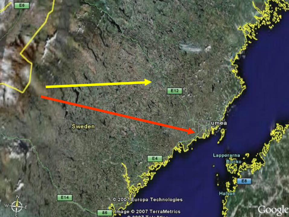
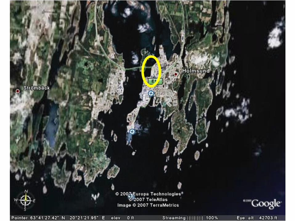
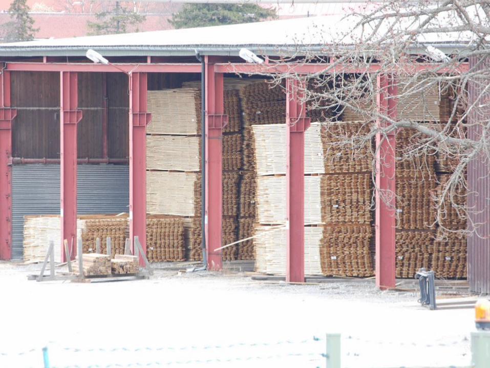
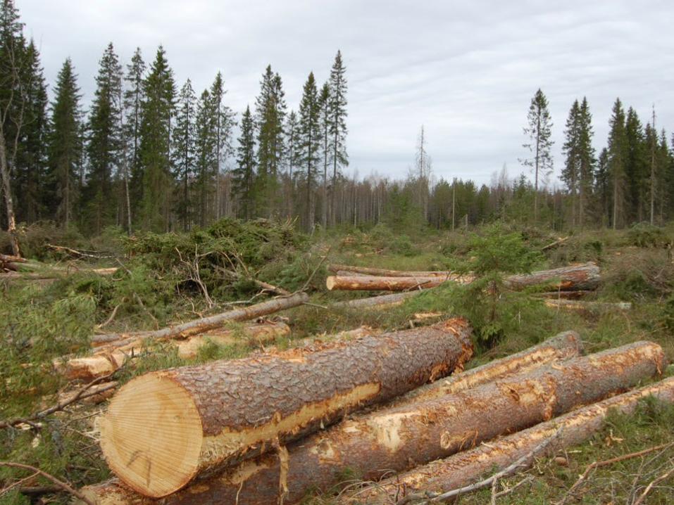
• A typical forest industry company is defined using real mills and forest conditions in the North of Sweden.
• For each year (or other period) and possible price and stock state, the variable company profit is maximized using linear programming. (Quadratic programming etc. are other options.)
• The expected present value of the company over an infinite horizon is maximized via stochastic dynamic programming in Markov chains. In this stage, a standard LP solver is used.

5

6
7

8

9

10

11

12
13

14

15

16
17
18

19
20

21
22
23

24

25

26

27

28
29

30
31

32

33

34

35

36
37

38

39

40

41

42
Optimization of the variable profit during a year:
Linear programming code
Background:
http://www.lohmander.com/SkogIndEk1/SI1.html

43
! SMB2;! Peter Lohmander 2003-10-15;
Max = TProf;TProf = - InkK - IntKostn + ForsI;InkK = PKTi*KTimmer + PKMav*KMav + PKFlis*KFlis + PReturpL*KReturpl + PReturpI*KReturpI; IntKostn = AvvK*Avv + TPKostTI*ETimmer + TPKostMA*EMav + CSV*ProdSV + CLiner*ProdLin;ForsI = PSV*ProdSV + PLiner*ProdLin + PSTi*STimmer + PSMav*SMav + PSFlis*SFlis;
!Market prices of raw material and raw material constraints;PKTi = 380;PSTi = 330;PKMav = 200;PSMav = 120;PKFlis = 250;PSFlis = 150;PReturpL = 50;PReturpI = 730;[LRetP] KReturpL <= 100;

44
!SMBs forest and harvesting;AvvK = 70;AvvKap = 570;TimAndel = .5;[KapAvv] Avv <= AvvKap;
!Roundwood transport costs;TPKostTI = 60;TPKostMa = 70; !SMBs saw mill;PSV = 1500;CSV = 300;SVKap = 80;TTimmer = ETimmer + KTimmer;ProdSV = .5*TTimmer;ProdFl = .8*ProdSV;ProdSp = .2*ProdSV;[KapSV] ProdSV <= SVKap;

45
!SMBs raw material balance;EMav = (1-TimAndel)* Avv - SMav;ETimmer = Timandel*Avv - STimmer;EFlis = ProdFl - SFlis;
!SMBs liner mill;PLiner = 4900;CLiner = 1200;LinerKap = 400;TRetP = KReturpL + KReturpI;TFiber = EMav + EFlis + KMav + KFlis; ProdLin = .25*TFiber + .95*TRetP;[FFiberK] TFiber/TRetP >= 4;[KapLiner] ProdLin <= LinerKap;end

46
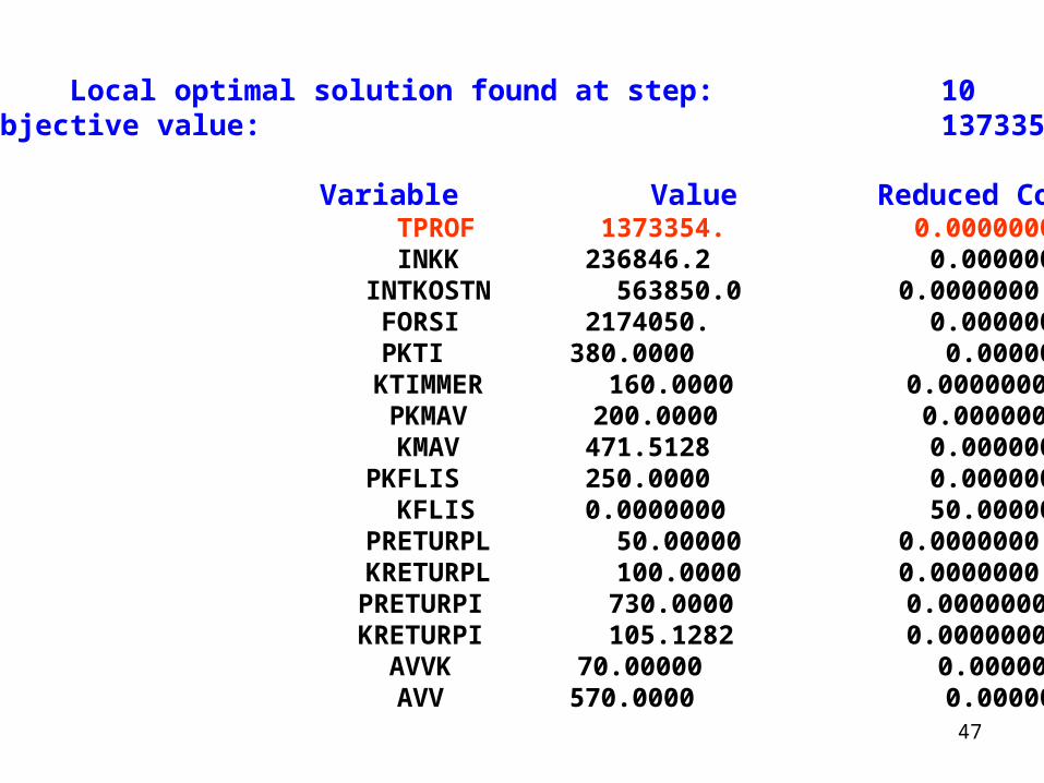
Optimization of the variable profit during a year:
Optimal results
47
Local optimal solution found at step: 10 Objective value: 1373354.
Variable Value Reduced Cost TPROF 1373354. 0.0000000 INKK 236846.2 0.0000000 INTKOSTN 563850.0 0.0000000 FORSI 2174050. 0.0000000 PKTI 380.0000 0.0000000 KTIMMER 160.0000 0.0000000 PKMAV 200.0000 0.0000000 KMAV 471.5128 0.0000000 PKFLIS 250.0000 0.0000000 KFLIS 0.0000000 50.00000
PRETURPL 50.00000 0.0000000 KRETURPL 100.0000 0.0000000 PRETURPI 730.0000 0.0000000 KRETURPI 105.1282 0.0000000 AVVK 70.00000 0.0000000 AVV 570.0000 0.0000000

48
TPKOSTTI 60.00000 0.0000000 ETIMMER 0.0000000 10.00000
TPKOSTMA 70.00000 0.0000000 EMAV 285.0000 0.0000000 CSV 300.0000 0.0000000
PRODSV 80.00000 0.0000000 CLINER 1200.000 0.0000000 PRODLIN 400.0000 0.0000000
PSV 1500.000 0.0000000 PLINER 4900.000 0.0000000 PSTI 330.0000 0.0000000
STIMMER 285.0000 0.0000000 PSMAV 120.0000 0.0000000 SMAV 0.0000000 10.00000 PSFLIS 150.0000 0.0000000 SFLIS 0.0000000 50.00000
AVVKAP 570.0000 0.0000000 TIMANDEL 0.5000000 0.0000000
SVKAP 80.00000 0.0000000
49
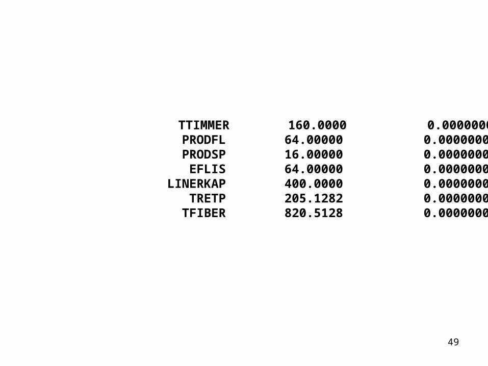
TTIMMER 160.0000 0.0000000 PRODFL 64.00000 0.0000000 PRODSP 16.00000 0.0000000 EFLIS 64.00000 0.0000000
LINERKAP 400.0000 0.0000000 TRETP 205.1282 0.0000000 TFIBER 820.5128 0.0000000

50
Row Slack or Surplus Dual PriceLRETP 0.0000000 680.0000KAPAVV 0.0000000 160.0000KAPSV 0.0000000 600.0000FFIBERK 0.6043397E-09 -788.9547KAPLINER 0.0000000 2915.385

51
”Single period results”
In the ”single period optimization model”, you should always harvest all
available stands and produce at full capacity utilization in the saw mill and the liner mill.
52
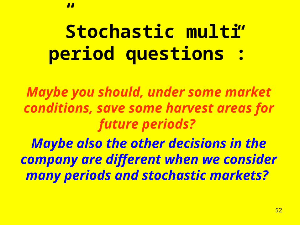
”Stochastic multi period questions”:
Maybe you should, under some market conditions, save some harvest areas for
future periods?
Maybe also the other decisions in the company are different when we consider many periods and stochastic markets?

53
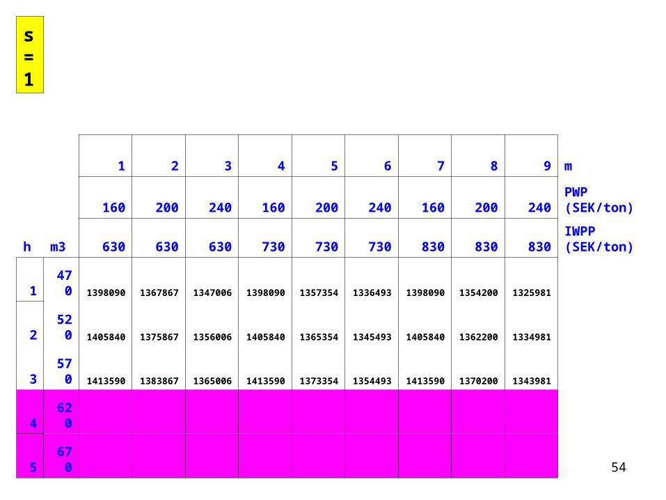
Optimal variable profit (KSEK/Year) as a function of * stock level * harvest level * price of external pulpwood (PWP)* price of imported waste paper (IWPP):
54
s = 1
1 2 3 4 5 6 7 8 9 m
160 200 240 160 200 240 160 200 240PWP (SEK/ton)
h m3 630 630 630 730 730 730 830 830 830IWPP (SEK/ton)
1 470 1398090 1367867 1347006 1398090 1357354 1336493 1398090 1354200 1325981
2 520 1405840 1375867 1356006 1405840 1365354 1345493 1405840 1362200 1334981
3 570 1413590 1383867 1365006 1413590 1373354 1354493 1413590 1370200 1343981
4 620
5 670
55
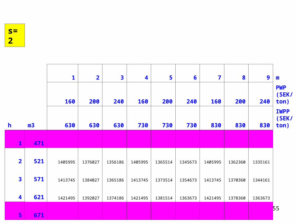
s=2
1 2 3 4 5 6 7 8 9 m
160 200 240 160 200 240 160 200 240
PWP (SEK/ton)
h m3 630 630 630 730 730 730 830 830 830
IWPP (SEK/ton)
1 471
2 521 1405995 1376027 1356186 1405995 1365514 1345673 1405995 1362360 1335161
3 571 1413745 1384027 1365186 1413745 1373514 1354673 1413745 1370360 1344161
4 621 1421495 1392027 1374186 1421495 1381514 1363673 1421495 1378360 1363673
5 671

56
s=3
1 2 3 4 5 6 7 8 9 m
160 200 240 160 200 240 160 200 240
PWP (SEK/ton)
h m3 630 630 630 730 730 730 830 830 830
IWPP (SEK/ton)
1 472
2 522
3 572 1413900 1384187 1365366 1413900 1373674 1354853 1413900 1370520 1344341
4 622 1421650 1392187 1374366 1421650 1381674 1363853 1421650 1378520 1353341
5 672 1429400 1400187 1383366 1429400 1389674 1372853 1429400 1386520 1362341

57
Optimization of the expected present value of the company
during over an infinite horizon:
Linear programming in a Markov chain

58
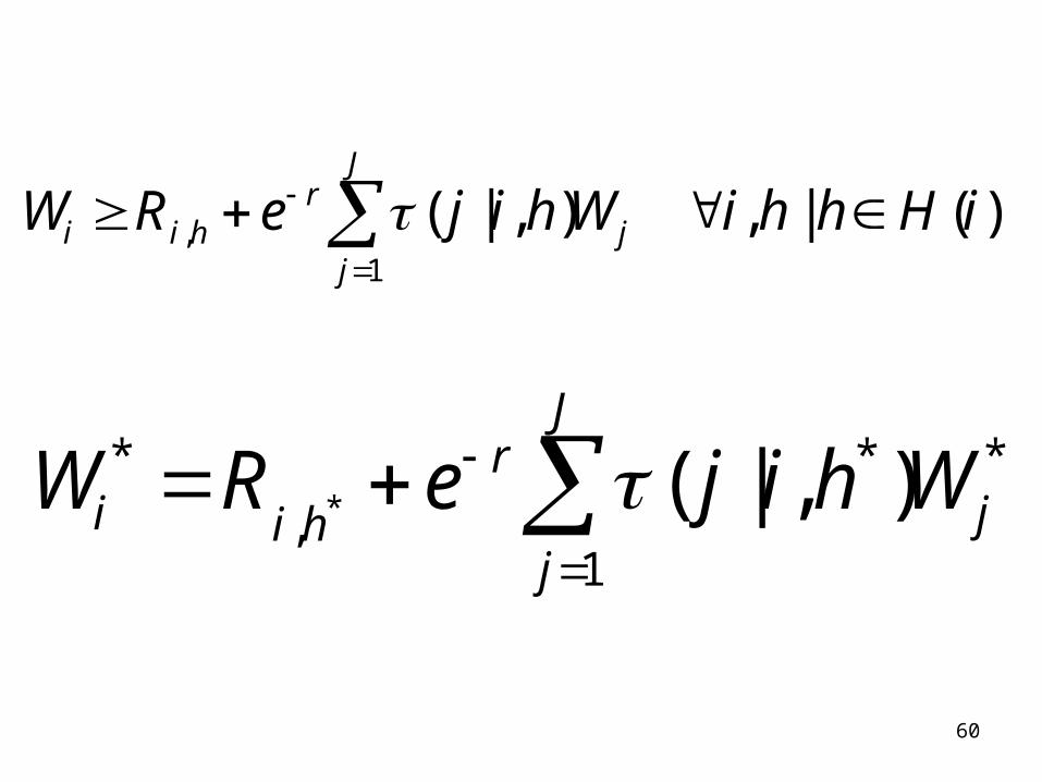
The optimization problem at a general level
We want to maximize the expected present value of the profit, all revenues minus costs, over an infinite horizon.
This is solved via stochastic dynamic programming. Compare Howard (1960),
Wagner (1975), Ross (1983) and Winston (2004).

59
* *
1
( , ) ( , , ) ( | , , ) ( , 1)max
( )
Jr
j
W i t R i t h e j i t h W j thh H i
60
,1
( | , ) , | ( )J
ri i h j
j
W R e j i h W i h h H i
*
* * *
,1
( | , )J
ri ji h
j
W R e j i h W
61
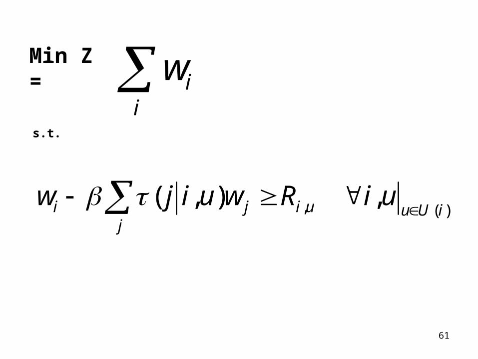
Min Z =
ii
w s.t.
, ( )( , ) ,i j i u u U i
j
w j i u w R i u

62
1
( )i
Z w i

63
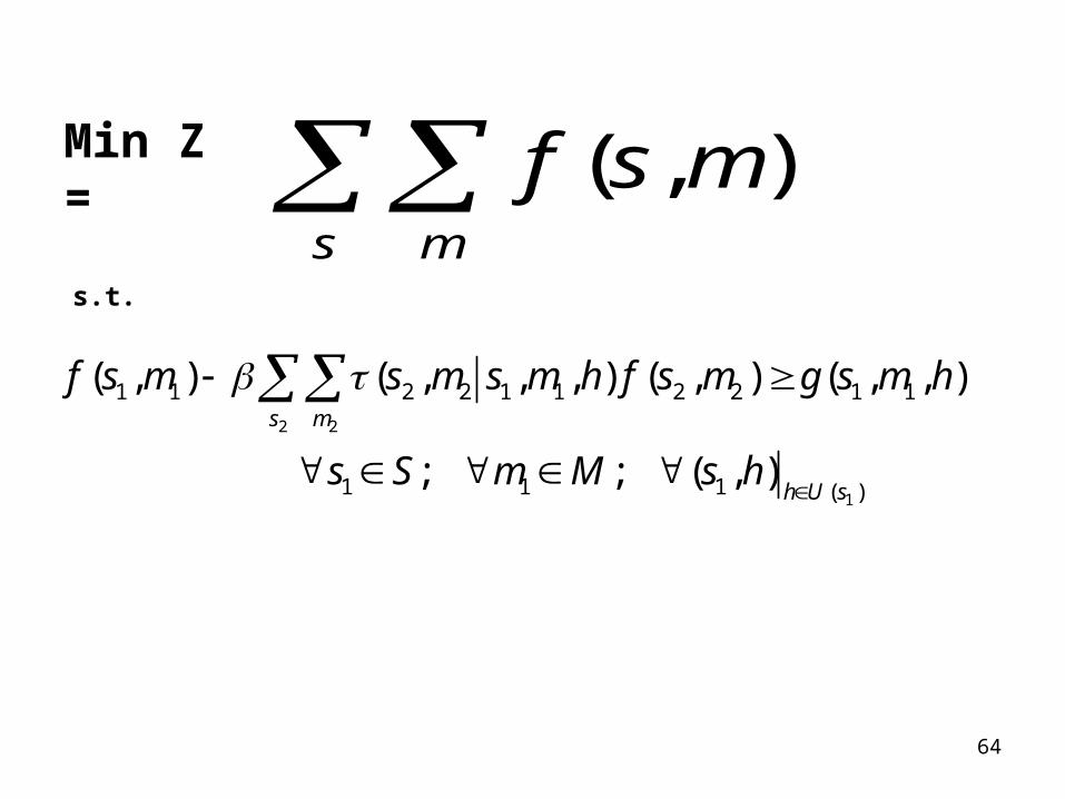
min ( , )s m
Z f s m
64
Min Z =
s.t.
2 2
1
1 1 2 2 1 1 2 2 1 1
1 1 1 ( )
( , ) ( , , , ) ( , ) ( , , )
; ; ( , )
s m
h U s
f s m s m s m h f s m g s m h
s S m M s h
( , )s m
f s m
65
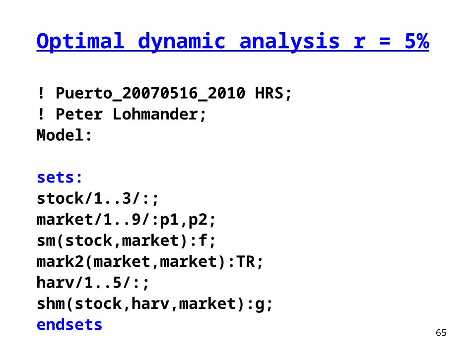
Optimal dynamic analysis r = 5%
! Puerto_20070516_2010 HRS;! Peter Lohmander;Model:
sets:stock/1..3/:;market/1..9/:p1,p2;sm(stock,market):f;mark2(market,market):TR;harv/1..5/:;shm(stock,harv,market):g;endsets

66
b = 1/1.05; Z = @sum( sm(i,j):f(i,j));min = Z;@for(stock(s): @for(market(m): @for(harv(h)| (s+3-h) #GE#1 #AND# (s+3-h) #LE# 3 :[Dec] f(s,m) >= g(s,h,m) + b*@sum(market(n):TR(m,n)*f(s+3-h,n)) )));

67
@for(mark2(m,n)| n #NE# 5 :
TR(m,n) = .05);
@for(mark2(m,n)| n #EQ# 5 :
TR(m,n) = .6);

68
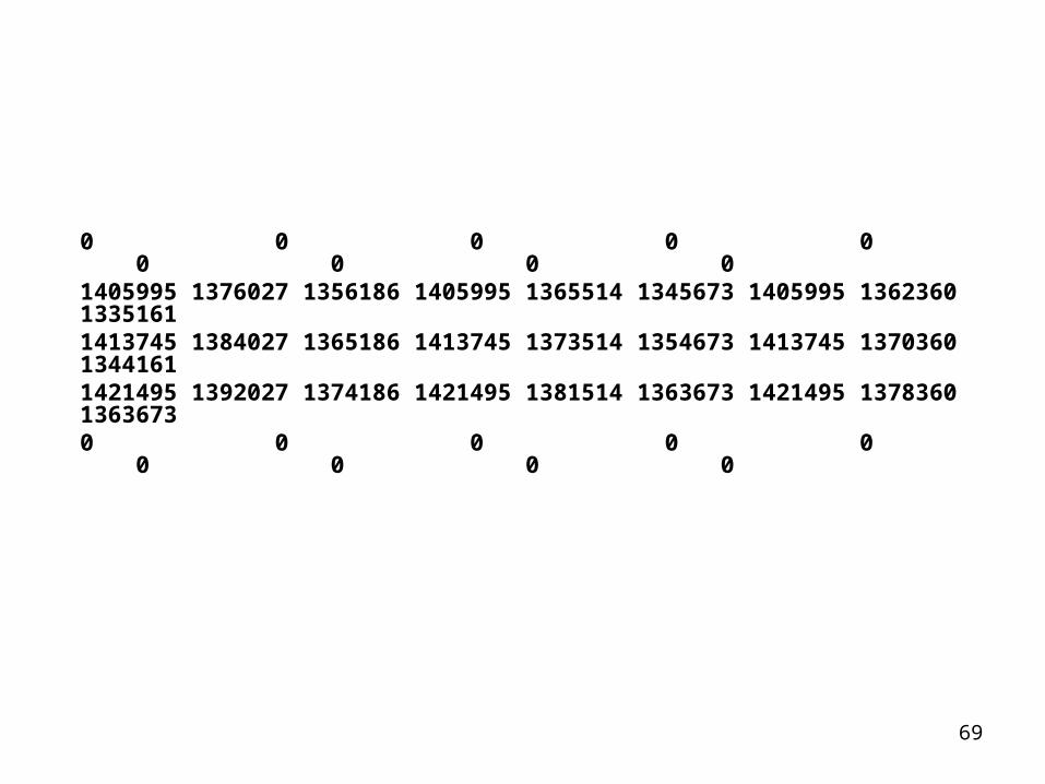
data:
g =
1398090 1367867 1347006 1398090 1357354 1336493 1398090 1354200 1325981
1405840 1375867 1356006 1405840 1365354 1345493 1405840 1362200 1334981
1413590 1383867 1365006 1413590 1373354 1354493 1413590 1370200 1343981
0 0 0 0 0 0 0 0 0
0 0 0 0 0 0 0 0 0
69
0 0 0 0 0 0 0 0 01405995 1376027 1356186 1405995 1365514 1345673 1405995 1362360 13351611413745 1384027 1365186 1413745 1373514 1354673 1413745 1370360 13441611421495 1392027 1374186 1421495 1381514 1363673 1421495 1378360 13636730 0 0 0 0 0 0 0 0

70
0 0 0 0 0 0 0 0 00 0 0 0 0 0 0 0 01413900 1384187 1365366 1413900 1373674 1354853 1413900 1370520 13443411421650 1392187 1374366 1421650 1381674 1363853 1421650 1378520 13533411429400 1400187 1383366 1429400 1389674 1372853 1429400 1386520 1362341 ;
p1 = 1 2 3 1 2 3 1 2 3;p2 = 1 1 1 2 2 2 3 3 3;
enddataend

71
Global optimal solution found at step: 94
Objective value: 0.7812784E+09

72
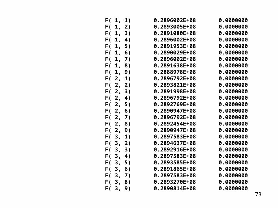
Variable Value Reduced Cost B 0.9523810 0.0000000 Z 0.7812784E+09 0.0000000
73
F( 1, 1) 0.2896002E+08 0.0000000 F( 1, 2) 0.2893005E+08 0.0000000 F( 1, 3) 0.2891080E+08 0.0000000 F( 1, 4) 0.2896002E+08 0.0000000 F( 1, 5) 0.2891953E+08 0.0000000 F( 1, 6) 0.2890029E+08 0.0000000 F( 1, 7) 0.2896002E+08 0.0000000 F( 1, 8) 0.2891638E+08 0.0000000 F( 1, 9) 0.2888978E+08 0.0000000 F( 2, 1) 0.2896792E+08 0.0000000 F( 2, 2) 0.2893821E+08 0.0000000 F( 2, 3) 0.2891998E+08 0.0000000 F( 2, 4) 0.2896792E+08 0.0000000 F( 2, 5) 0.2892769E+08 0.0000000 F( 2, 6) 0.2890947E+08 0.0000000 F( 2, 7) 0.2896792E+08 0.0000000 F( 2, 8) 0.2892454E+08 0.0000000 F( 2, 9) 0.2890947E+08 0.0000000 F( 3, 1) 0.2897583E+08 0.0000000 F( 3, 2) 0.2894637E+08 0.0000000 F( 3, 3) 0.2892916E+08 0.0000000 F( 3, 4) 0.2897583E+08 0.0000000 F( 3, 5) 0.2893585E+08 0.0000000 F( 3, 6) 0.2891865E+08 0.0000000 F( 3, 7) 0.2897583E+08 0.0000000 F( 3, 8) 0.2893270E+08 0.0000000 F( 3, 9) 0.2890814E+08 0.0000000

74
F( 1, 5) 0.2891953E+08 0.0000000

75
F( 1, 5) 0.2891953E+08 0.0000000F( 2, 5) 0.2892769E+08 0.0000000F( 3, 5) 0.2893585E+08 0.0000000
76
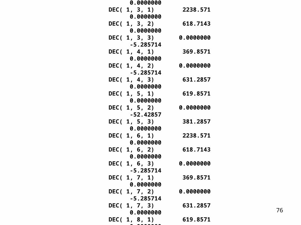
DEC( 1, 1, 1) 369.8571 0.0000000 DEC( 1, 1, 2) 0.0000000 -5.285714 DEC( 1, 1, 3) 631.2857 0.0000000 DEC( 1, 2, 1) 619.8571 0.0000000 DEC( 1, 2, 2) 0.0000000 -5.285714 DEC( 1, 2, 3) 381.2857 0.0000000 DEC( 1, 3, 1) 2238.571 0.0000000 DEC( 1, 3, 2) 618.7143 0.0000000 DEC( 1, 3, 3) 0.0000000 -5.285714 DEC( 1, 4, 1) 369.8571 0.0000000 DEC( 1, 4, 2) 0.0000000 -5.285714 DEC( 1, 4, 3) 631.2857 0.0000000 DEC( 1, 5, 1) 619.8571 0.0000000 DEC( 1, 5, 2) 0.0000000 -52.42857 DEC( 1, 5, 3) 381.2857 0.0000000 DEC( 1, 6, 1) 2238.571 0.0000000 DEC( 1, 6, 2) 618.7143 0.0000000 DEC( 1, 6, 3) 0.0000000 -5.285714 DEC( 1, 7, 1) 369.8571 0.0000000 DEC( 1, 7, 2) 0.0000000 -5.285714 DEC( 1, 7, 3) 631.2857 0.0000000 DEC( 1, 8, 1) 619.8571 0.0000000 DEC( 1, 8, 2) 0.0000000 -5.285714 DEC( 1, 8, 3) 381.2857 0.0000000 DEC( 1, 9, 1) 2238.571 0.0000000 DEC( 1, 9, 2) 618.7143 0.0000000 DEC( 1, 9, 3) 0.0000000 -5.285714

77
DEC( 1, 5, 1) 619.8571 0.0000000 DEC( 1, 5, 2) 0.0000000 -52.42857 DEC( 1, 5, 3) 381.2857 0.0000000

78
DEC( 2, 1, 2) 369.8571 0.0000000 DEC( 2, 1, 3) 0.0000000 -23.71428 DEC( 2, 1, 4) 631.2857 0.0000000 DEC( 2, 2, 2) 619.8571 0.0000000 DEC( 2, 2, 3) 0.0000000 -23.71428 DEC( 2, 2, 4) 381.2857 0.0000000 DEC( 2, 3, 2) 2238.571 0.0000000 DEC( 2, 3, 3) 618.7143 0.0000000 DEC( 2, 3, 4) 0.0000000 -23.71428 DEC( 2, 4, 2) 369.8571 0.0000000 DEC( 2, 4, 3) 0.0000000 -23.71428 DEC( 2, 4, 4) 631.2857 0.0000000 DEC( 2, 5, 2) 619.8571 0.0000000 DEC( 2, 5, 3) 0.0000000 -273.5714 DEC( 2, 5, 4) 381.2857 0.0000000 DEC( 2, 6, 2) 2238.571 0.0000000 DEC( 2, 6, 3) 618.7143 0.0000000 DEC( 2, 6, 4) 0.0000000 -23.71428 DEC( 2, 7, 2) 369.8571 0.0000000 DEC( 2, 7, 3) 0.0000000 -23.71428 DEC( 2, 7, 4) 631.2857 0.0000000 DEC( 2, 8, 2) 619.8571 0.0000000 DEC( 2, 8, 3) 0.0000000 -23.71428 DEC( 2, 8, 4) 381.2857 0.0000000 DEC( 2, 9, 2) 12750.57 0.0000000 DEC( 2, 9, 3) 11130.71 0.0000000 DEC( 2, 9, 4) 0.0000000 -23.71428
79
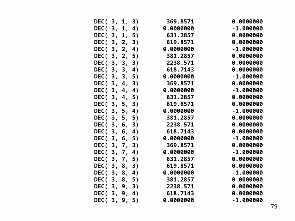
DEC( 3, 1, 3) 369.8571 0.0000000 DEC( 3, 1, 4) 0.0000000 -1.000000 DEC( 3, 1, 5) 631.2857 0.0000000 DEC( 3, 2, 3) 619.8571 0.0000000 DEC( 3, 2, 4) 0.0000000 -1.000000 DEC( 3, 2, 5) 381.2857 0.0000000 DEC( 3, 3, 3) 2238.571 0.0000000 DEC( 3, 3, 4) 618.7143 0.0000000 DEC( 3, 3, 5) 0.0000000 -1.000000 DEC( 3, 4, 3) 369.8571 0.0000000 DEC( 3, 4, 4) 0.0000000 -1.000000 DEC( 3, 4, 5) 631.2857 0.0000000 DEC( 3, 5, 3) 619.8571 0.0000000 DEC( 3, 5, 4) 0.0000000 -1.000000 DEC( 3, 5, 5) 381.2857 0.0000000 DEC( 3, 6, 3) 2238.571 0.0000000 DEC( 3, 6, 4) 618.7143 0.0000000 DEC( 3, 6, 5) 0.0000000 -1.000000 DEC( 3, 7, 3) 369.8571 0.0000000 DEC( 3, 7, 4) 0.0000000 -1.000000 DEC( 3, 7, 5) 631.2857 0.0000000 DEC( 3, 8, 3) 619.8571 0.0000000 DEC( 3, 8, 4) 0.0000000 -1.000000 DEC( 3, 8, 5) 381.2857 0.0000000 DEC( 3, 9, 3) 2238.571 0.0000000 DEC( 3, 9, 4) 618.7143 0.0000000 DEC( 3, 9, 5) 0.0000000 -1.000000
80
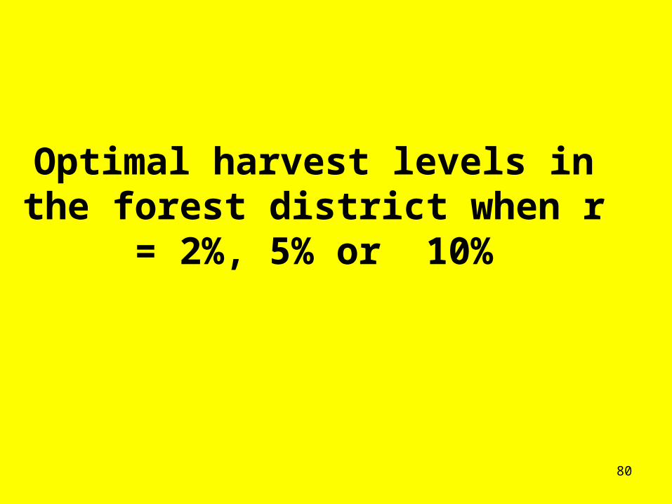
Optimal harvest levels in the forest district when r = 2%, 5% or
10%

81
S = Entering stock level S=1 (570 000 m3 or less may be harvested this year)
PWP = 160 PWP = 200 PWP = 240
IWPP = 830 520 000 m3 520 000 m3 570 000 m3
IWPP = 730 520 000 m3 520 000 m3 570 000 m3
IWPP = 630 520 000 m3 520 000 m3 570 000 m3
Optimal harvest levels in the forest district when r = 2%, 5% or 10%

82
Optimal harvest levels in the forest district when r = 2%, 5% or 10%
S=2 (621 000 m3 or less may be harvested this year)
PWP = 160 PWP = 200 PWP = 240
IWPP = 830 571 000 m3 571 000 m3 621 000 m3
IWPP = 730 571 000 m3 571 000 m3 621 000 m3
IWPP = 630 571 000 m3 571 000 m3 621 000 m3

83
Optimal harvest levels in the forest district when r = 2%, 5% or 10%
S=3 (672 000 m3 or less may be harvested this year)
PWP = 160 PWP = 200 PWP = 240
IWPP = 830 622 000 m3 622 000 m3 672 000 m3
IWPP = 730 622 000 m3 622 000 m3 672 000 m3
IWPP = 630 622 000 m3 622 000 m3 672 000 m3

84
Optimal harvest levels in the forest district when r = 2%, 5% or
10%:
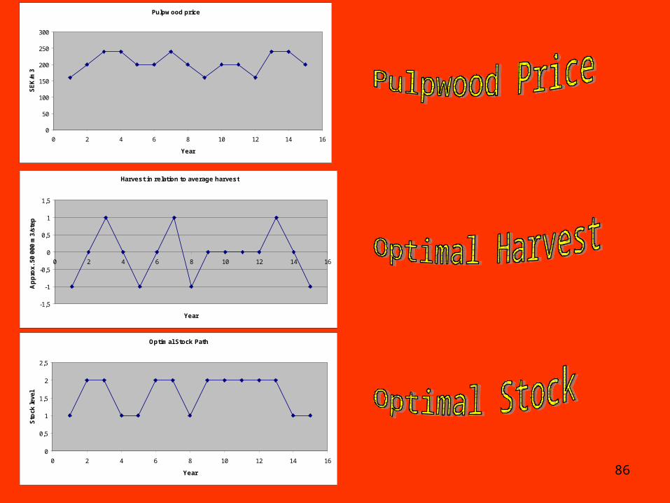
Harvest approx. 50 000 cubic metres less than the maximum possible in case the pulp wood price is not at the highest level. Harvest as much as possible if
the pulp wood price is at the highest level.
85
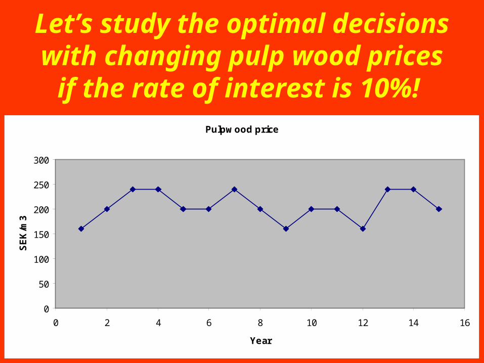
Pulpwood price
0
50
100
150
200
250
300
0 2 4 6 8 10 12 14 16
Year
SE
K/m
3Let’s study the optimal decisions with changing pulp wood prices
if the rate of interest is 10%!
86
Pulpwood price
0
50
100
150
200
250
300
0 2 4 6 8 10 12 14 16
Year
SE
K/m
3
Harvest in relation to average harvest
-1,5
-1
-0,5
0
0,5
1
1,5
0 2 4 6 8 10 12 14 16
Year
Ap
pro
x. 5
0 00
0 m
3/st
ep
Optimal Stock Path
0
0,5
1
1,5
2
2,5
0 2 4 6 8 10 12 14 16
Year
Sto
ck le
vel

87
Optimal harvest levels in the forest district when r = 15% (or
higher)

88
S = Entering stock level S=1 (570 000 m3 or less may be harvested this year)
Optimal harvest levels in the forest district when r = 15%
PWP = 160 PWP = 200 PWP = 240
IWPP = 830 570 000 m3 570 000 m3 570 000 m3
IWPP = 730 570 000 m3 570 000 m3 570 000 m3
IWPP = 630 570 000 m3 570 000 m3 570 000 m3
89
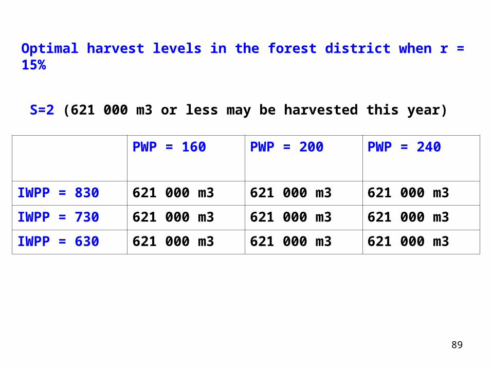
Optimal harvest levels in the forest district when r = 15%
S=2 (621 000 m3 or less may be harvested this year)
PWP = 160 PWP = 200 PWP = 240
IWPP = 830 621 000 m3 621 000 m3 621 000 m3
IWPP = 730 621 000 m3 621 000 m3 621 000 m3
IWPP = 630 621 000 m3 621 000 m3 621 000 m3

90
Optimal harvest levels in the forest district when r = 15%
S=3 (672 000 m3 or less may be harvested this year)
PWP = 160 PWP = 200 PWP = 240
IWPP = 830 672 000 m3 672 000 m3 672 000 m3
IWPP = 730 672 000 m3 672 000 m3 672 000 m3
IWPP = 630 672 000 m3 672 000 m3 672 000 m3

91
Optimal harvest levels in the forest district when r = 15% (or
higher):
Harvest as much as possible for all possible pulp wood prices!

92
General results• With this approach, all relevant decisions in
the company can be consistently optimized.• For instance, we find how the optimal
harvest level is affected by the present price in the pulpwood market, the transition probability matrix of prices, the rate of interest, the volume of harvestable stands and all other company relevant conditions such as capacities in the sawmill, the liner mill, transport costs for different assortements on different roads etc..
93
Observation #1All the sub problems (the
optimization problems within each time period) may be solved with
continuous or discrete variables via linear programming, quadratic programming or some other
optimization method, taking all relevant constraints into
consideration.

94
Observation #2In the ”master problem” (the Markov chain problem over an infinite horizon), the state space is discrete. With standard software,
this still makes it possible to use high resolution in the interesting dimensions.
For instance, with ten possible stock levels, we may use four exogenous market prices
(with ten possible levels in each dimension) and still have no more than 100 000
variables. Such a problem can easily be solved.
95
Observation #3This forest sector model can easily be
modified and we can instantly calculate how the expected economic value of the
company and the optimal decisions change.
For instance, we may introduce ”possible”
bioenergy power plants and new types of pulp and paper mills and instantly derive
the optimal results.

96
Abstract
• Forest industry production, capacity and harvest levels are optimized.
• Adaptive full system optimization is necessary for consistent results.
• The stochastic dynamic programming problem of a complete forest industry company is solved. The raw material stock level and the main product prices are state variables. In each state and at each stage, a linear programming profit maximization problem of the forest company is solved. Parameters from the Swedish forest industry are used as illustration.

97

98
Contact: Peter Lohmander
Professor
SLU, Dept. of Forest Economics
SE-901 83 Umea, Sweden
e-mail:
Personal home page:
http://www.Lohmander.com