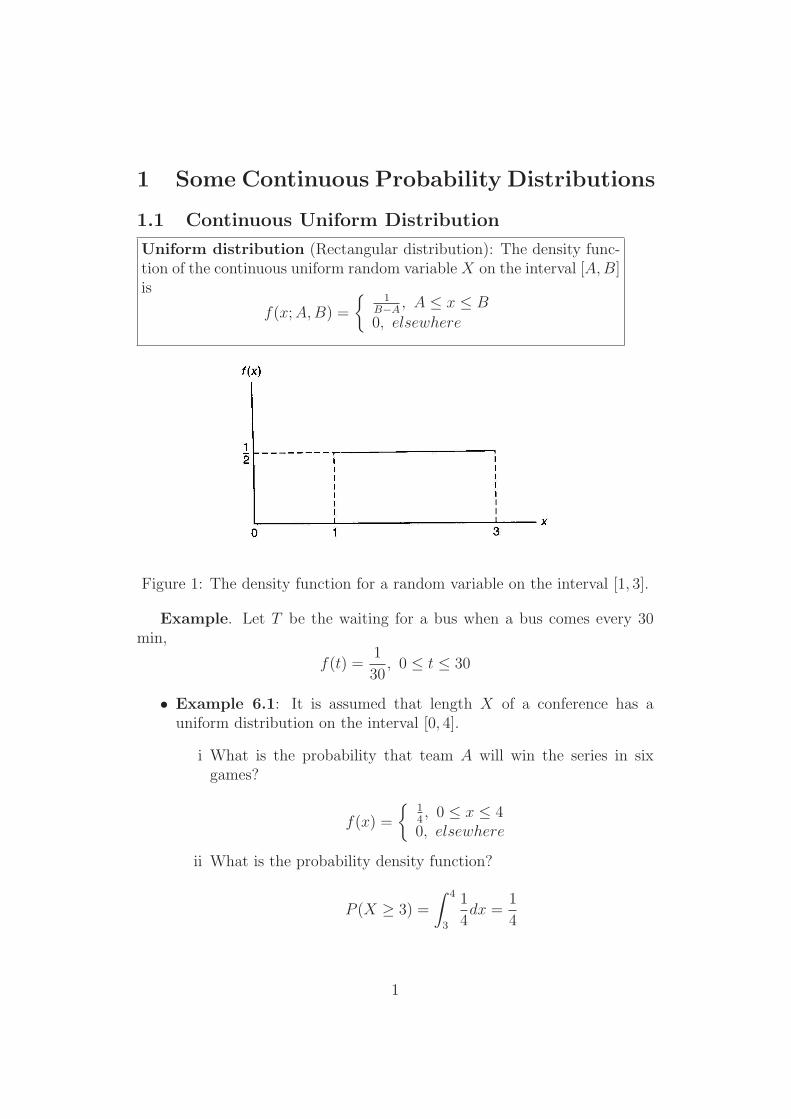
1 Some Continuous Probability Distributions

1.1 Continuous Uniform Distribution

Uniform distribution (Rectangular distribution): The density func-tion of the continuous uniform random variable X on the interval [A,B]is

f(x; A,B) =

{

1B−A

, A ≤ x ≤ B

0, elsewhere

Figure 1: The density function for a random variable on the interval [1, 3].

Example. Let T be the waiting for a bus when a bus comes every 30min,

f(t) =1

30, 0 ≤ t ≤ 30

• Example 6.1: It is assumed that length X of a conference has auniform distribution on the interval [0, 4].

i What is the probability that team A will win the series in sixgames?

f(x) =

{

14, 0 ≤ x ≤ 4

0, elsewhere

ii What is the probability density function?

P (X ≥ 3) =

∫ 4

3

1

4dx =

1

4

1

• Theorem 6.1:The mean and variance of the uniform distribution are

µ =A + B

2, σ2 =

(B − A)2

12

• Mean is at the center of the range as we would expect.

1.2 Normal Distribution

• The most important continuous probability distribution in the entirefield of statistics is the normal distribution.

• The normal curve describes approximately many phenomena thatoccur in nature, industry and research (human height, measurementerrors, stock market!, etc.).

• In 1733, Abraham DeMoivre developed the mathematical equation ofthe normal curve.

• The normal distribution is often referred to as the Gaussian distribu-

tion, in honour of Karl Friedrich Gauss (1777-1855), who also derivedits equation from a study of errors in repeated measurements of thesame quantity.

• The term normal distribution is a historical accident because there isnothing particularly normal about the normal distribution and nor isthere anything abnormal about other distribution.

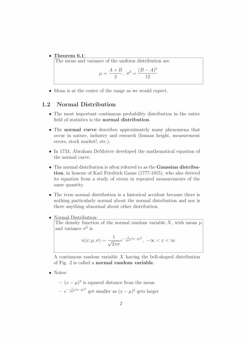
• Normal Distribution:The density function of the normal random variable X, with mean µ

and variance σ2 is

n(x; µ, σ) =1√2πσ

e−1

2σ2(x−µ)2 , −∞ < x < ∞

A continuous random variable X having the bell-shaped distributionof Fig. 2 is called a normal random variable.

• Notes:

– (x − µ)2 is squared distance from the mean

– e−1

2σ2(x−µ)2 get smaller as (x − µ)2 gets larger

2

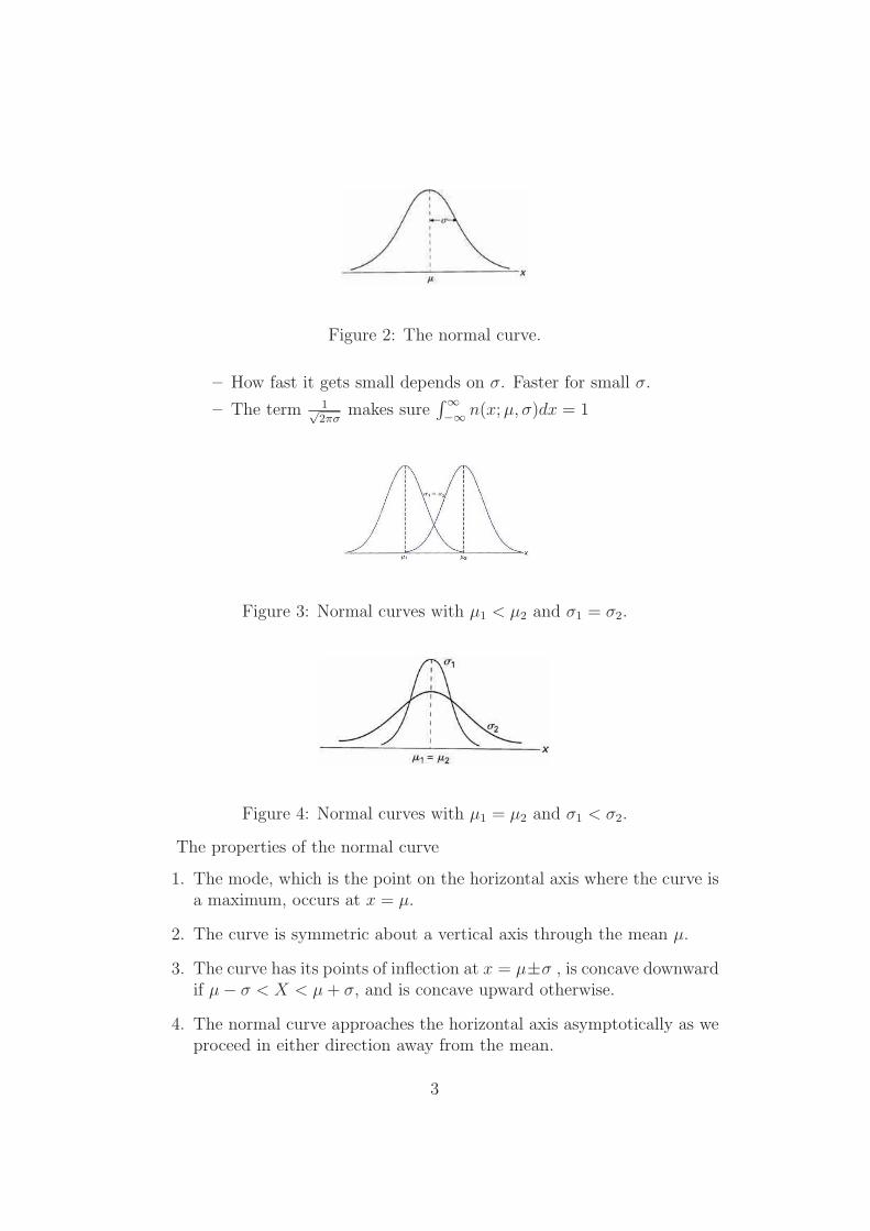
Figure 2: The normal curve.

– How fast it gets small depends on σ. Faster for small σ.

– The term 1√2πσ

makes sure∫ ∞

−∞n(x; µ, σ)dx = 1

Figure 3: Normal curves with µ1 < µ2 and σ1 = σ2.

Figure 4: Normal curves with µ1 = µ2 and σ1 < σ2.

The properties of the normal curve

1. The mode, which is the point on the horizontal axis where the curve isa maximum, occurs at x = µ.

2. The curve is symmetric about a vertical axis through the mean µ.

3. The curve has its points of inflection at x = µ±σ , is concave downwardif µ − σ < X < µ + σ, and is concave upward otherwise.

4. The normal curve approaches the horizontal axis asymptotically as weproceed in either direction away from the mean.

3

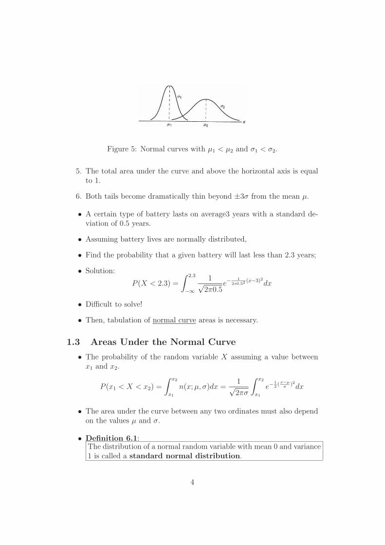
Figure 5: Normal curves with µ1 < µ2 and σ1 < σ2.

5. The total area under the curve and above the horizontal axis is equalto 1.

6. Both tails become dramatically thin beyond ±3σ from the mean µ.

• A certain type of battery lasts on average3 years with a standard de-viation of 0.5 years.

• Assuming battery lives are normally distributed,

• Find the probability that a given battery will last less than 2.3 years;

• Solution:

P (X < 2.3) =

∫ 2.3

−∞

1√2π0.5

e−1

2∗0.52(x−3)2dx

• Difficult to solve!

• Then, tabulation of normal curve areas is necessary.

1.3 Areas Under the Normal Curve

• The probability of the random variable X assuming a value betweenx1 and x2.

P (x1 < X < x2) =

∫ x2

x1

n(x; µ, σ)dx =1√2πσ

∫ x2

x1

e−1

2(x−µ

σ)2dx

• The area under the curve between any two ordinates must also dependon the values µ and σ.

• Definition 6.1:The distribution of a normal random variable with mean 0 and variance1 is called a standard normal distribution.

4

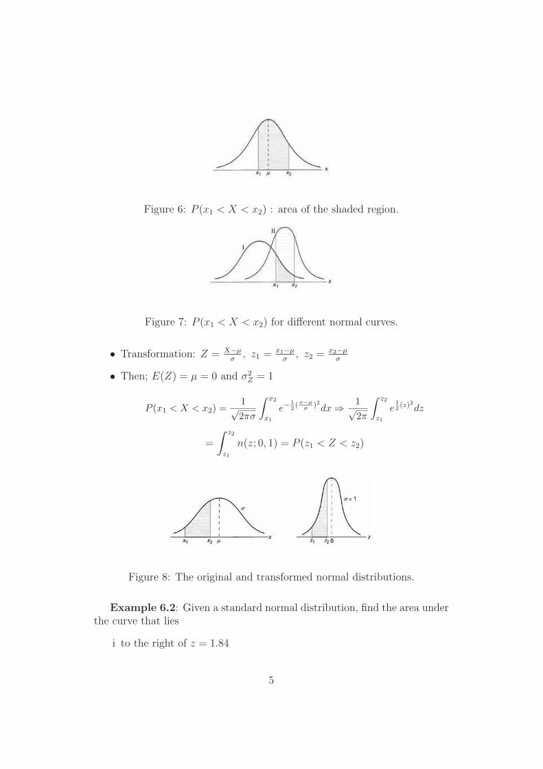
Figure 6: P (x1 < X < x2) : area of the shaded region.

Figure 7: P (x1 < X < x2) for different normal curves.

• Transformation: Z = X−µ

σ, z1 = x1−µ

σ, z2 = x2−µ

σ

• Then; E(Z) = µ = 0 and σ2Z = 1

P (x1 < X < x2) =1√2πσ

∫ x2

x1

e−1

2(x−µ

σ)2dx ⇒

1√2π

∫ z2

z1

e1

2(z)2dz

=

∫ z2

z1

n(z; 0, 1) = P (z1 < Z < z2)

Figure 8: The original and transformed normal distributions.

Example 6.2: Given a standard normal distribution, find the area underthe curve that lies

i to the right of z = 1.84

5

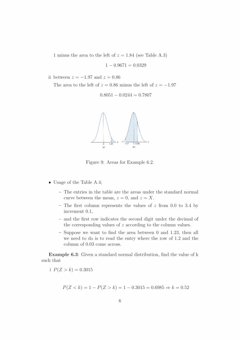
1 minus the area to the left of z = 1.84 (see Table A.3)

1 − 0.9671 = 0.0329

ii between z = −1.97 and z = 0.86

The area to the left of z = 0.86 minus the left of z = −1.97

0.8051 − 0.0244 = 0.7807

Figure 9: Areas for Example 6.2.

• Usage of the Table A.4;

– The entries in the table are the areas under the standard normalcurve between the mean, z = 0, and z = X.

– The first column represents the values of z from 0.0 to 3.4 byincrement 0.1,

– and the first row indicates the second digit under the decimal ofthe corresponding values of z according to the column values.

– Suppose we want to find the area between 0 and 1.23, then allwe need to do is to read the entry where the row of 1.2 and thecolumn of 0.03 come across.

Example 6.3: Given a standard normal distribution, find the value of ksuch that

i P (Z > k) = 0.3015

P (Z < k) = 1 − P (Z > k) = 1 − 0.3015 = 0.6985 ⇒ k = 0.52

6

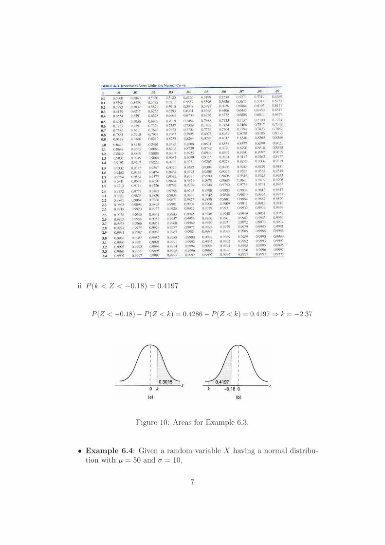
ii P (k < Z < −0.18) = 0.4197

P (Z < −0.18) − P (Z < k) = 0.4286 − P (Z < k) = 0.4197 ⇒ k = −2.37

Figure 10: Areas for Example 6.3.

• Example 6.4: Given a random variable X having a normal distribu-tion with µ = 50 and σ = 10,

7

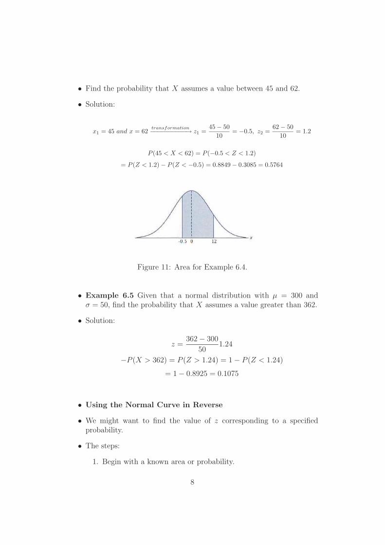
• Find the probability that X assumes a value between 45 and 62.

• Solution:

x1 = 45 and x = 62transformation−−−−−−−−−−→ z1 =

45 − 50

10= −0.5, z2 =

62 − 50

10= 1.2

P (45 < X < 62) = P (−0.5 < Z < 1.2)

= P (Z < 1.2) − P (Z < −0.5) = 0.8849 − 0.3085 = 0.5764

Figure 11: Area for Example 6.4.

• Example 6.5 Given that a normal distribution with µ = 300 andσ = 50, find the probability that X assumes a value greater than 362.

• Solution:

z =362 − 300

501.24

−P (X > 362) = P (Z > 1.24) = 1 − P (Z < 1.24)

= 1 − 0.8925 = 0.1075

• Using the Normal Curve in Reverse

• We might want to find the value of z corresponding to a specifiedprobability.

• The steps:

1. Begin with a known area or probability.

8

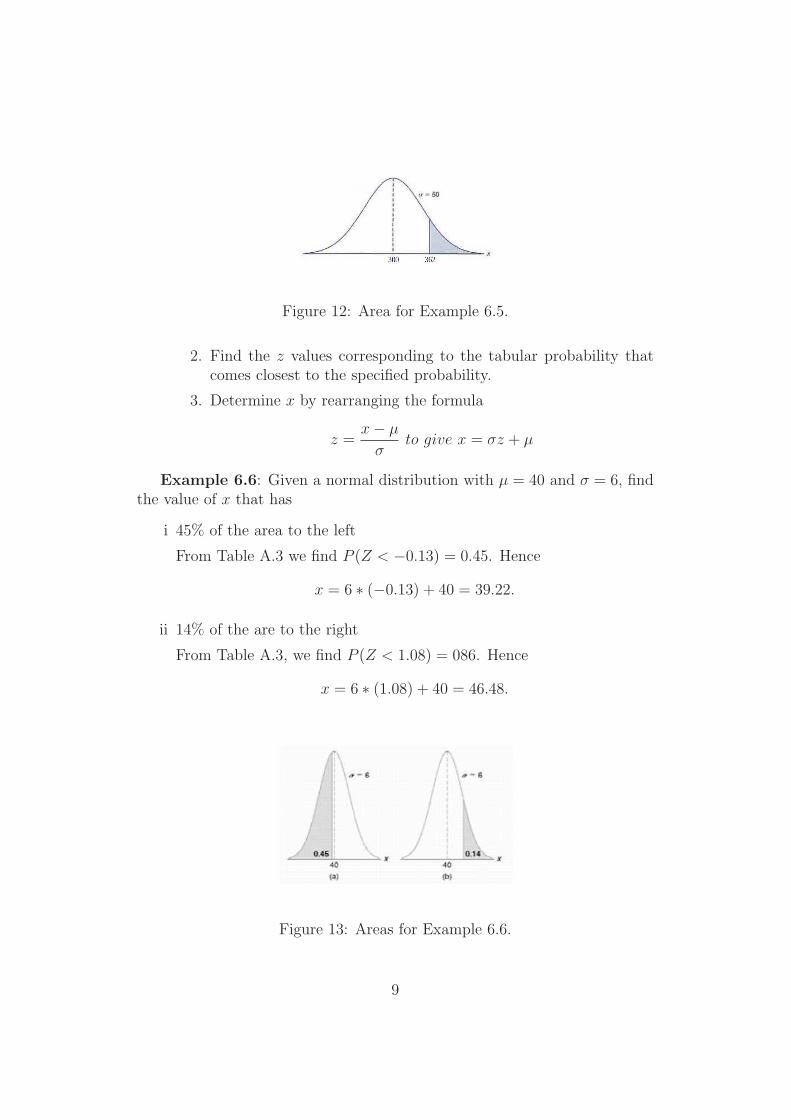
Figure 12: Area for Example 6.5.

2. Find the z values corresponding to the tabular probability thatcomes closest to the specified probability.

3. Determine x by rearranging the formula

z =x − µ

σto give x = σz + µ

Example 6.6: Given a normal distribution with µ = 40 and σ = 6, findthe value of x that has

i 45% of the area to the left

From Table A.3 we find P (Z < −0.13) = 0.45. Hence

x = 6 ∗ (−0.13) + 40 = 39.22.

ii 14% of the are to the right

From Table A.3, we find P (Z < 1.08) = 086. Hence

x = 6 ∗ (1.08) + 40 = 46.48.

Figure 13: Areas for Example 6.6.

9

1.4 Applications of the Normal Distribution

• Some of the many problems for which the normal distribution is appli-cable are treated in the following examples.

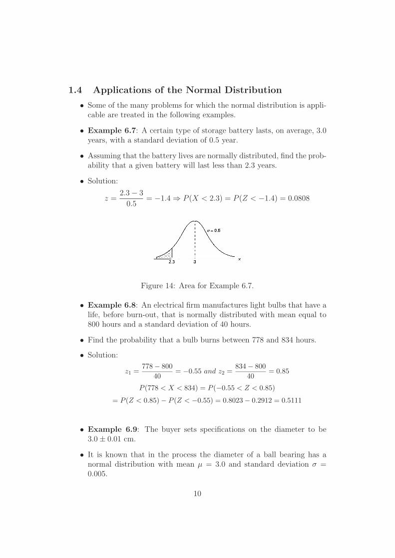
• Example 6.7: A certain type of storage battery lasts, on average, 3.0years, with a standard deviation of 0.5 year.

• Assuming that the battery lives are normally distributed, find the prob-ability that a given battery will last less than 2.3 years.

• Solution:

z =2.3 − 3

0.5= −1.4 ⇒ P (X < 2.3) = P (Z < −1.4) = 0.0808

Figure 14: Area for Example 6.7.

• Example 6.8: An electrical firm manufactures light bulbs that have alife, before burn-out, that is normally distributed with mean equal to800 hours and a standard deviation of 40 hours.

• Find the probability that a bulb burns between 778 and 834 hours.

• Solution:

z1 =778 − 800

40= −0.55 and z2 =

834 − 800

40= 0.85

P (778 < X < 834) = P (−0.55 < Z < 0.85)

= P (Z < 0.85) − P (Z < −0.55) = 0.8023 − 0.2912 = 0.5111

• Example 6.9: The buyer sets specifications on the diameter to be3.0 ± 0.01 cm.

• It is known that in the process the diameter of a ball bearing has anormal distribution with mean µ = 3.0 and standard deviation σ =0.005.

10

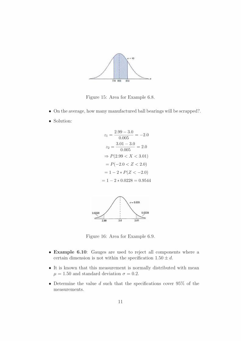
Figure 15: Area for Example 6.8.

• On the average, how many manufactured ball bearings will be scrapped?.

• Solution:

z1 =2.99 − 3.0

0.005= −2.0

z2 =3.01 − 3.0

0.005= 2.0

⇒ P (2.99 < X < 3.01)

= P (−2.0 < Z < 2.0)

= 1 − 2 ∗ P (Z < −2.0)

= 1 − 2 ∗ 0.0228 = 0.9544

Figure 16: Area for Example 6.9.

• Example 6.10: Gauges are used to reject all components where acertain dimension is not within the specification 1.50 ± d.

• It is known that this measurement is normally distributed with meanµ = 1.50 and standard deviation σ = 0.2.

• Determine the value d such that the specifications cover 95% of themeasurements.

11

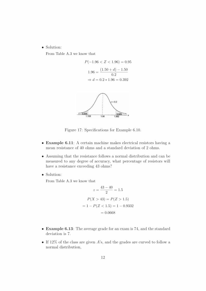
• Solution:

From Table A.3 we know that

P (−1.96 < Z < 1.96) = 0.95

1.96 =(1.50 + d) − 1.50

0.2

⇒ d = 0.2 ∗ 1.96 = 0.392

Figure 17: Specifications for Example 6.10.

• Example 6.11: A certain machine makes electrical resistors having amean resistance of 40 ohms and a standard deviation of 2 ohms.

• Assuming that the resistance follows a normal distribution and can bemeasured to any degree of accuracy, what percentage of resistors willhave a resistance exceeding 43 ohms?

• Solution:

From Table A.3 we know that

z =43 − 40

2= 1.5

P (X > 43) = P (Z > 1.5)

= 1 − P (Z < 1.5) = 1 − 0.9332

= 0.0668

• Example 6.13: The average grade for an exam is 74, and the standarddeviation is 7.

• If 12% of the class are given A’s, and the grades are curved to follow anormal distribution,

12

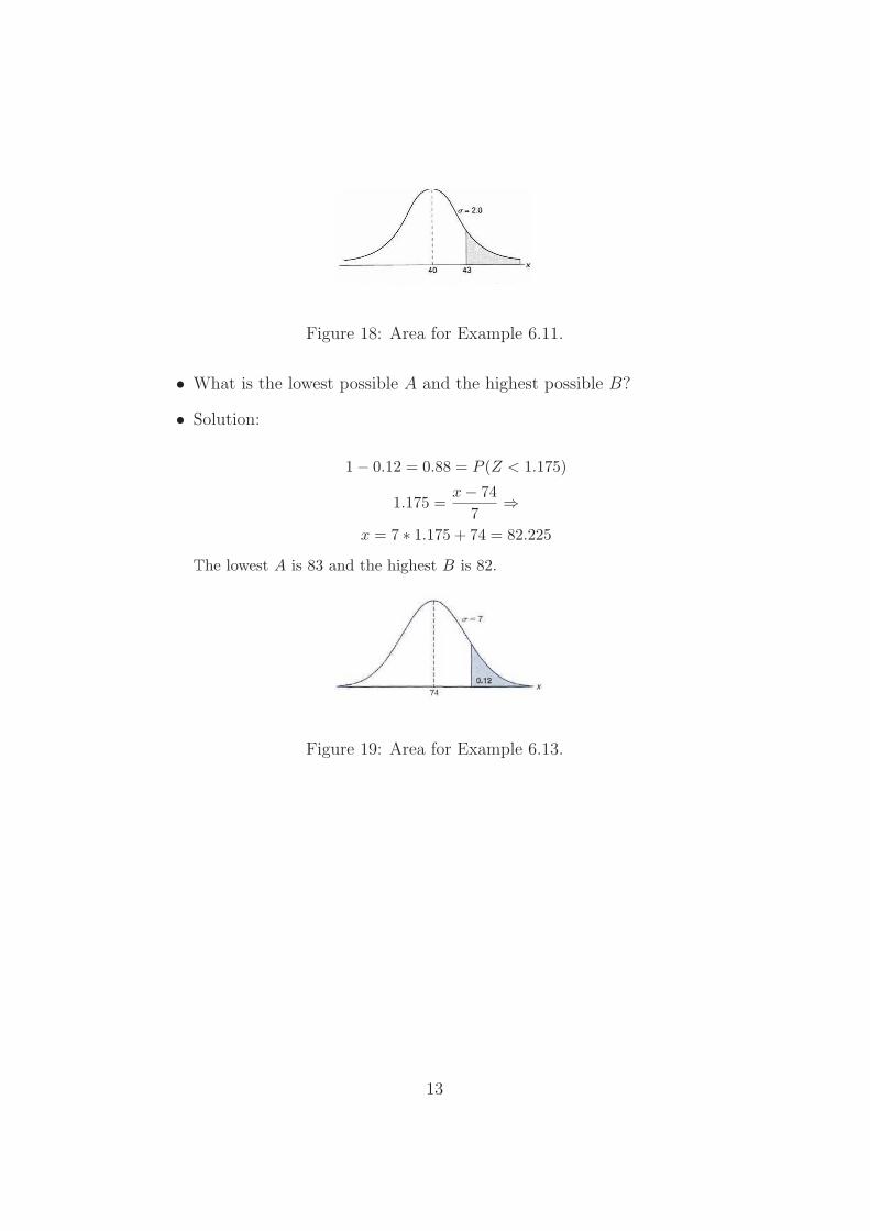
Figure 18: Area for Example 6.11.

• What is the lowest possible A and the highest possible B?

• Solution:

1 − 0.12 = 0.88 = P (Z < 1.175)

1.175 =x − 74

7⇒

x = 7 ∗ 1.175 + 74 = 82.225

The lowest A is 83 and the highest B is 82.

Figure 19: Area for Example 6.13.

13