5/3/01 Sudeshna Sarkar, CSE, IIT Kharagpur1 Structures Lecture 21 5.3.2001.
Upload
kathryn-blankenshipCategory
view
216download
1
1
Sequence Learning
Sudeshna Sarkar
14 Aug 2008
2
Alternative graphical models for part of speech tagging
3
Different Models for POS tagging
HMM
Maximum Entropy Markov Models
Conditional Random Fields

4
Hidden Markov Model (HMM) : Generative Modeling
Source Model PY
Noisy Channel PXY
y x
i
ii yyPP )|()( 1y i
ii yxPP )|()|( yx

5
Dependency (1st order)
kY1kY
kX
)|( kk YXP
)|( 1kk YYP
1kX
)|( 11 kk YXP
2kX
)|( 22 kk YXP
2kY)|( 21 kk YYP
1kY
1kX
)|( 1 kk YYP
)|( 11 kk YXP
6
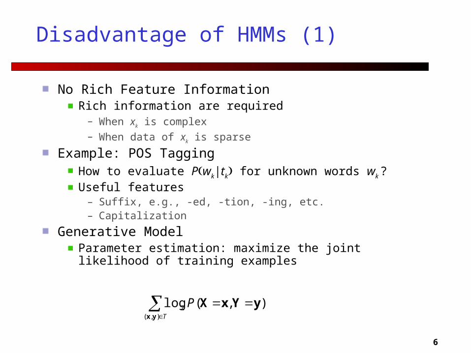
Disadvantage of HMMs (1)
No Rich Feature InformationRich information are required
– When xk is complex– When data of xk is sparse
Example: POS TaggingHow to evaluate Pwk|tk for unknown words wk ?Useful features
– Suffix, e.g., -ed, -tion, -ing, etc.– Capitalization
Generative ModelParameter estimation: maximize the joint likelihood of training examples
T
P),(
2 ),(logyx
yYxX
7
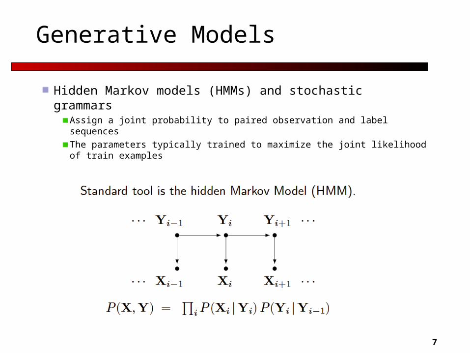
Generative Models
Hidden Markov models (HMMs) and stochastic grammarsAssign a joint probability to paired observation and label sequences
The parameters typically trained to maximize the joint likelihood of train examples
8
Generative Models (cont’d)
Difficulties and disadvantagesNeed to enumerate all possible observation sequences
Not practical to represent multiple interacting features or long-range dependencies of the observations
Very strict independence assumptions on the observations
9
Making use of rich domain features
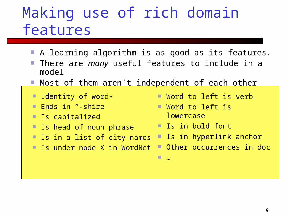
A learning algorithm is as good as its features.There are many useful features to include in a modelMost of them aren’t independent of each other
Identity of word
Ends in “-shire”
Is capitalized
Is head of noun phrase
Is in a list of city names
Is under node X in WordNet
Word to left is verb
Word to left is lowercase
Is in bold font
Is in hyperlink anchor
Other occurrences in doc
…
10
Problems with Richer Representationand a Generative Model
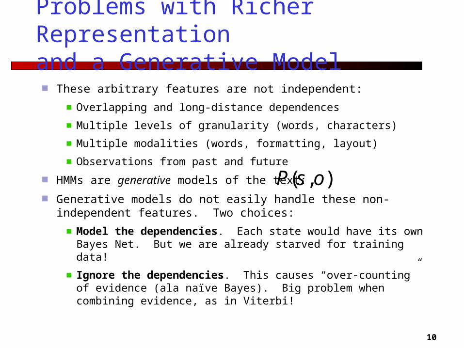
These arbitrary features are not independent:
Overlapping and long-distance dependences
Multiple levels of granularity (words, characters)
Multiple modalities (words, formatting, layout)
Observations from past and future
HMMs are generative models of the text:
Generative models do not easily handle these non-independent features. Two choices:
Model the dependencies. Each state would have its own Bayes Net. But we are already starved for training data!
Ignore the dependencies. This causes “over-counting” of evidence (ala naïve Bayes). Big problem when combining evidence, as in Viterbi!
),( osP
11
Discriminative Models
We would prefer a conditional model:P(y|x) instead of P(y,x):
Can examine features, but not responsible for generating them.
Don’t have to explicitly model their dependencies.
Don’t “waste modeling effort” trying to generate what we are given at test time anyway.
Provide the ability to handle many arbitrary features.
12
Locally Normalized Conditional Sequence Model
St -1
St
Ot
St+1
Ot +1
Ot -1
...
...
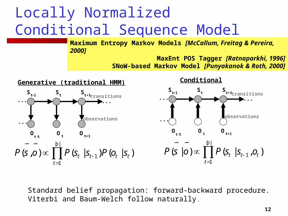
Generative (traditional HMM)
||
11 )|()|(),(
o
ttttt soPssPosP
...transitions
observations
St -1
St
Ot
St+1
Ot +1
Ot -1
...
...
Conditional
...transitions
observations
||
11 ),|()|(
o
tttt ossPosP
Standard belief propagation: forward-backward procedure.Viterbi and Baum-Welch follow naturally.
Maximum Entropy Markov Models [McCallum, Freitag & Pereira, 2000]MaxEnt POS Tagger [Ratnaparkhi, 1996]
SNoW-based Markov Model [Punyakanok & Roth, 2000]
13
Locally Normalized Conditional Sequence Model
St -1
St
Ot
St+1
Ot +1
Ot -1
...
...
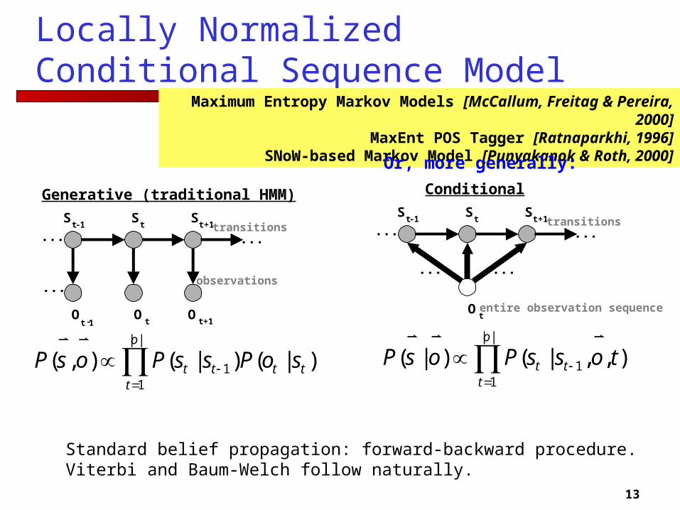
Generative (traditional HMM)
||
11 )|()|(),(
o
ttttt soPssPosP
...transitions
observations
St -1
St
Ot
St+1
...
...
Conditional
...transitions
entire observation sequence
||
11 ),,|()|(
o
ttt tossPosP
Standard belief propagation: forward-backward procedure.Viterbi and Baum-Welch follow naturally.
Maximum Entropy Markov Models [McCallum, Freitag & Pereira, 2000]MaxEnt POS Tagger [Ratnaparkhi, 1996]
SNoW-based Markov Model [Punyakanok & Roth, 2000]
Or, more generally:
...
14
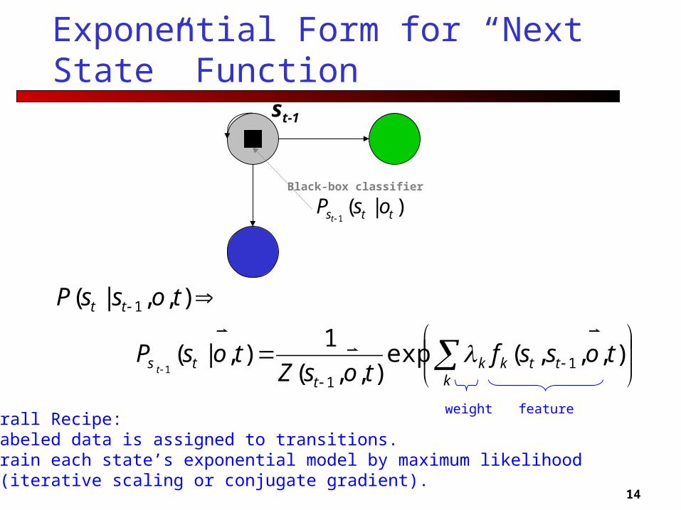
Exponential Form for “Next State” Function
k
ttkkt
ts
tt
tossftosZ
tosP
tossP
t),,,(exp
),,(
1),|(
),,|(
11
1
1
Overall Recipe:- Labeled data is assigned to transitions.- Train each state’s exponential model by maximum likelihood (iterative scaling or conjugate gradient).
weight feature
)|(1 tts osP
t
Black-box classifier
st-1
15
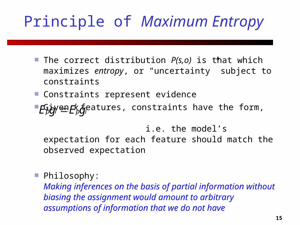
Principle of Maximum Entropy
The correct distribution P(s,o) is that which maximizes entropy, or “uncertainty” subject to constraints
Constraints represent evidence
Given k features, constraints have the form, i.e. the model’s expectation for each feature should match the observed expectation
Philosophy: Making inferences on the basis of partial information without biasing the assignment would amount to arbitrary assumptions of information that we do not have
p i p iE g E g
16
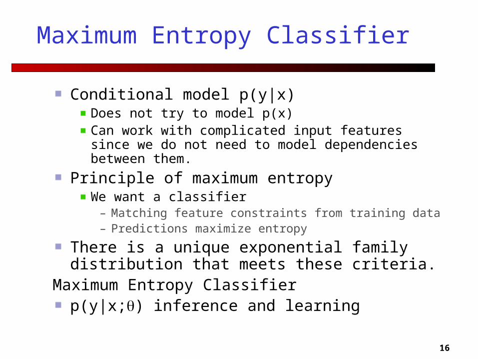
Maximum Entropy Classifier
Conditional model p(y|x)Does not try to model p(x)Can work with complicated input features since we do not need to model dependencies between them.
Principle of maximum entropyWe want a classifier
– Matching feature constraints from training data– Predictions maximize entropy
There is a unique exponential family distribution that meets these criteria.
Maximum Entropy Classifierp(y|x;) inference and learning
17
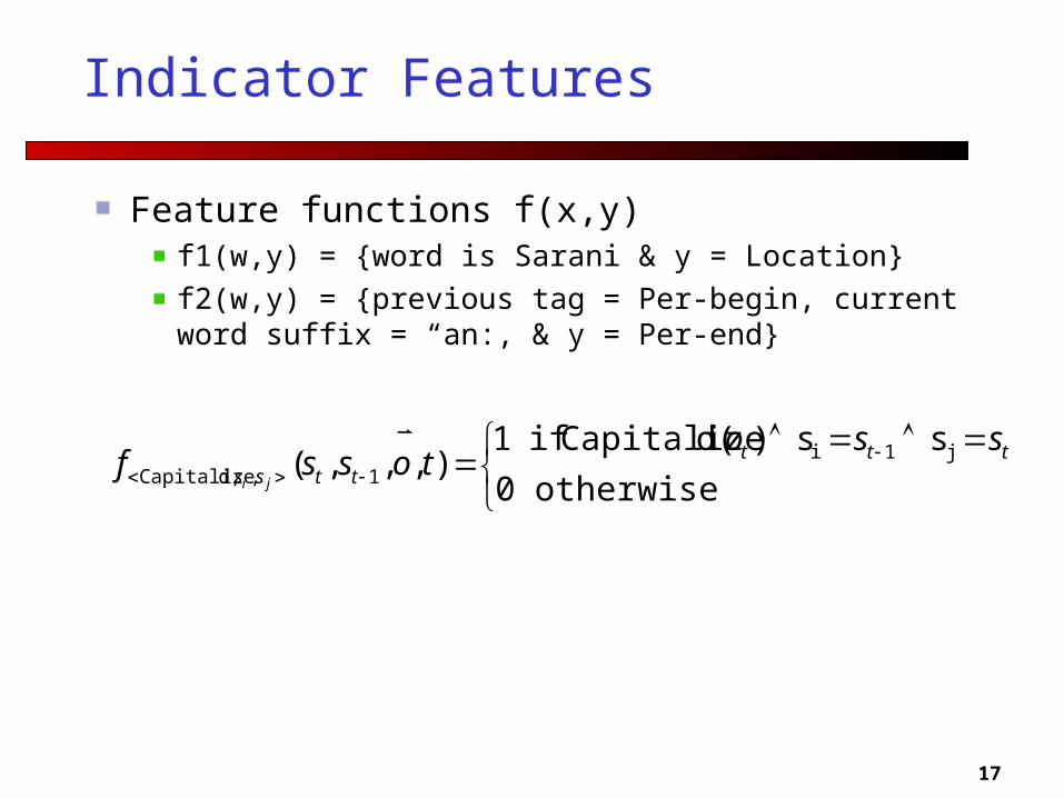
Indicator Features
Feature functions f(x,y)f1(w,y) = {word is Sarani & y = Location}
f2(w,y) = {previous tag = Per-begin, current word suffix = “an:, & y = Per-end}
otherwise 0
s s )d(Capitalize if 1),,,( j1i
1,d,Capitalizettt
ttss
ssotossf
ji

18
Problems with MaxEnt classifier
It makes decisions at each point independently

19
MEMM
Use a series of maximum entropy classifiers that know the previous labelDefine a Viterbi model of inference
P(y|x) = t Pyt-1 (yt|x)Finding the most likely label sequence given an input sequence and learningCombines the advantages of HMM and maximum entropy.But there is a problem.

20
Maximum Entropy Markov Model
n
iiii xsspxspxsp
2111 ),|()|()|(
Label bias problem: the probability transitions leaving any given state must sum to one
21
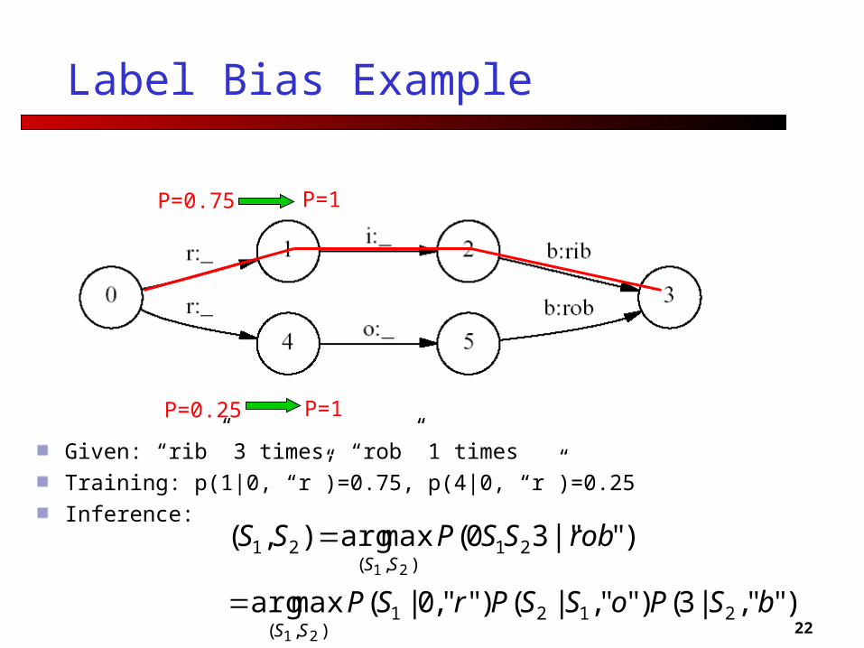
In some state space configurations, MEMMs essentially completely ignore the inputs
Example of label bias problem
This is not a problem for HMMs, because the input is generated by the model.
22
P=0.75
P=0.25
P=1
P=1
Label Bias Example
Given: “rib” 3 times, “rob” 1 times
Training: p(1|0, “r”)=0.75, p(4|0, “r”)=0.25
Inference:
)"",|3()"",|()"",0|(maxarg
)"|"30(maxarg),(
2121),(
21),(
21
21
21
bSPoSSPrSP
robSSPSS
SS
SS
23
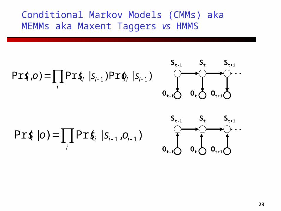
Conditional Markov Models (CMMs) aka MEMMs aka Maxent Taggers vs HMMS
St-1 St
Ot
St+1
Ot+1Ot-1
... i
iiii sossos )|Pr()|Pr(),Pr( 11
St-1 St
Ot
St+1
Ot+1Ot-1
...
i
iii ossos ),|Pr()|Pr( 11
24
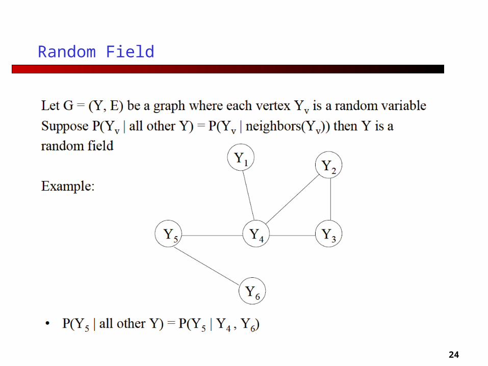
Random Field
25
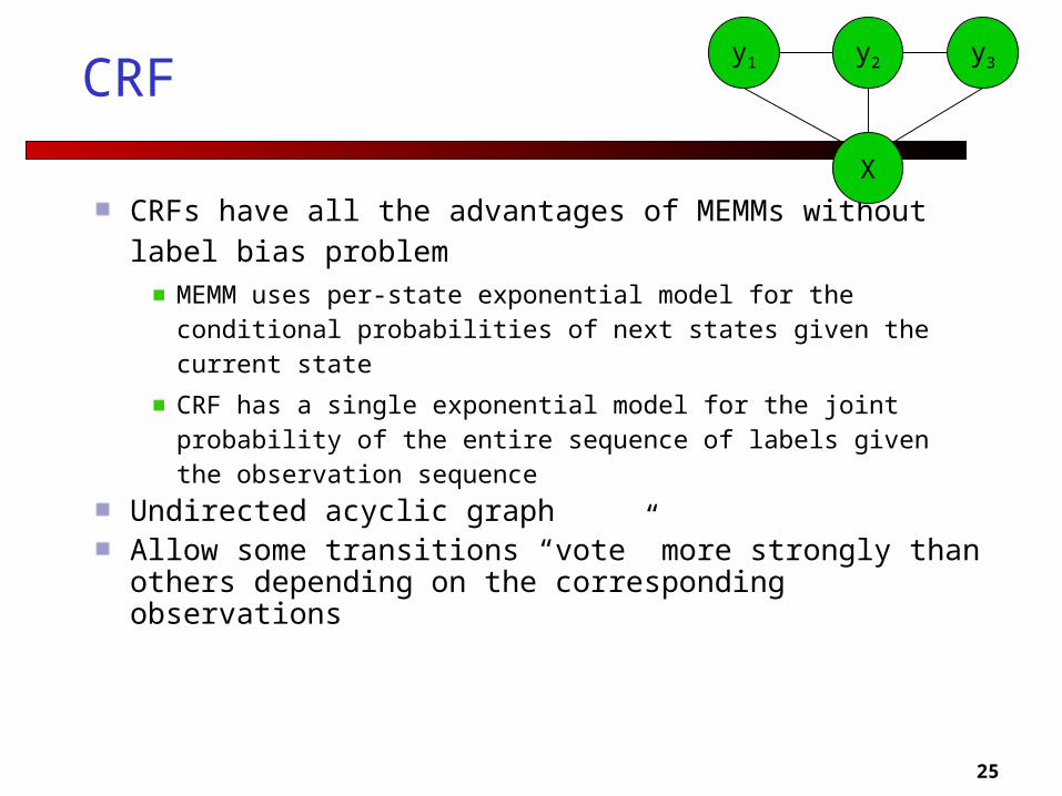
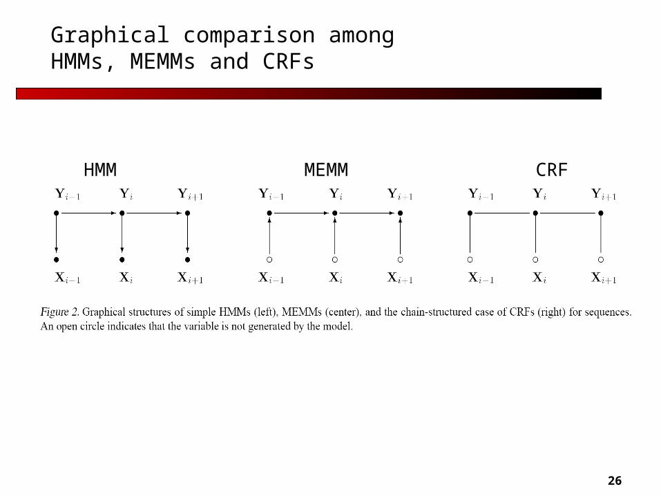
CRF
CRFs have all the advantages of MEMMs without label bias problem
MEMM uses per-state exponential model for the conditional probabilities of next states given the current state
CRF has a single exponential model for the joint probability of the entire sequence of labels given the observation sequence
Undirected acyclic graphAllow some transitions “vote” more strongly than others depending on the corresponding observations
X
y1 y2 y3
26
Graphical comparison among HMMs, MEMMs and CRFs
HMM MEMM CRF
27
Machine Learning a Panacea?
A machine learning method is as good as the feature set it uses
Shift focus from linguistic processing to feature set design
28
Features to use in IE
Features are task dependent
Good feature identification needs a good knowledge of the domain combined with automatic methods of feature selection.
29
Feature Examples
Extraction of protein and their interactions from biomedical literature (Mooney)
For each token, they take the following as features:
– Current token
– Last 2 tokens and next 2 tokens
– Output of dictionary-based tagger for these 5 tokens
– Suffix for each of the 5 tokens (last 1, 2, and 3 characters)
– Class labels for last 2 tokens
Two potentially oncogenic cyclins , cyclin A and cyclin D1 , share common properties of subunit configuration , tyrosine phosphorylation and physical association with the Rb protein
30
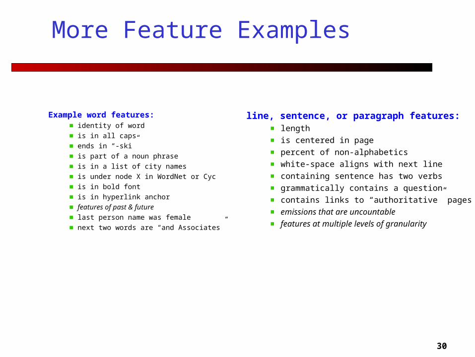
More Feature Examples
line, sentence, or paragraph features:length
is centered in page
percent of non-alphabetics
white-space aligns with next line
containing sentence has two verbs
grammatically contains a question
contains links to “authoritative” pages
emissions that are uncountable
features at multiple levels of granularity
Example word features:identity of word
is in all caps
ends in “-ski”
is part of a noun phrase
is in a list of city names
is under node X in WordNet or Cyc
is in bold font
is in hyperlink anchor
features of past & future
last person name was female
next two words are “and Associates”
31
Indicator Features
They’re a little different from the typical supervised ML approach
Limited to binary values– Think of a feature as being on or off rather than as a feature with a
value
Feature values are relative to an object/class pair rather than being a function of the object alone.Typically have lots and lots of features (100s of 1000s of features is quite common.)
32
Feature Templates
Next word
A feature template – gives rise to |V|x|T| binary features
Curse of Dimensionality
Overfitting
33
Feature Selection vs Extraction
Feature selection: Choosing k<d important features, ignoring the remaining d – k
Subset selection algorithms
Feature extraction: Project the
original xi , i =1,...,d dimensions to
new k<d dimensions, zj , j =1,...,k
Principal components analysis (PCA), linear discriminant analysis (LDA), factor analysis (FA)
34
Feature Reduction
Example domain: NER in Hindi (Sujan Saha)
Feature Value Selection
Feature Value Clustering
ACL 2008: Kumar Saha; Pabitra Mitra; Sudeshna SarkarWord Clustering and Word Selection Based Feature Reduction for MaxEnt Based Hindi NER

35
36
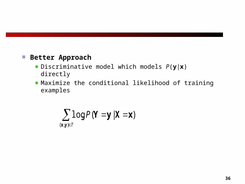
Better ApproachDiscriminative model which models P(y|x) directly
Maximize the conditional likelihood of training examples
T
P),(
2 )|(logyx
xXyY
37
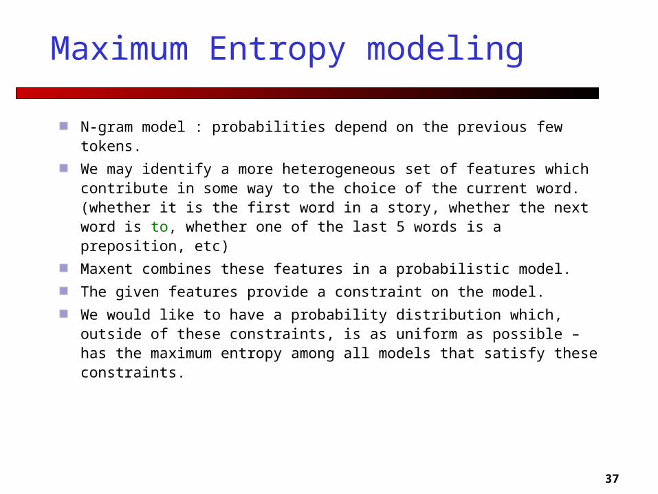
Maximum Entropy modeling
N-gram model : probabilities depend on the previous few tokens.
We may identify a more heterogeneous set of features which contribute in some way to the choice of the current word. (whether it is the first word in a story, whether the next word is to, whether one of the last 5 words is a preposition, etc)
Maxent combines these features in a probabilistic model.
The given features provide a constraint on the model.
We would like to have a probability distribution which, outside of these constraints, is as uniform as possible – has the maximum entropy among all models that satisfy these constraints.
38
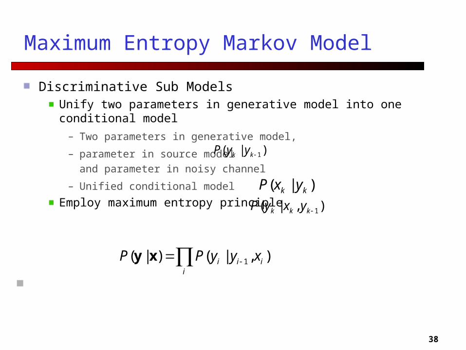
Maximum Entropy Markov Model
Discriminative Sub ModelsUnify two parameters in generative model into one conditional model
– Two parameters in generative model,
– parameter in source model and parameter in noisy
channel
– Unified conditional model
Employ maximum entropy principle
)|( 1kk yyP
)|( kk yxP ),|( 1kkk yxyP
i
iii xyyPP ),|()|( 1xy
Maximum Entropy Markov Model

39
General Maximum Entropy Principle
Model
Model distribution PY|X with a set of features fffl defined on X and Y
IdeaCollect information of features from training data
Principle
– Model what is known
– Assume nothing else
Flattest distribution
Distribution with the maximum Entropy
40
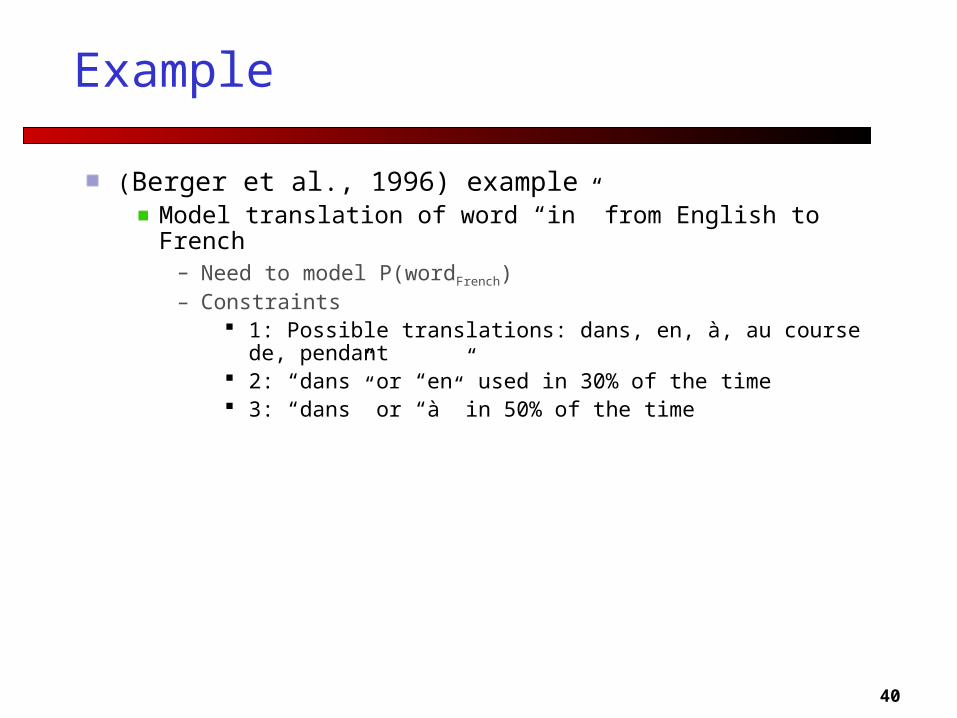
Example
(Berger et al., 1996) exampleModel translation of word “in” from English to French
– Need to model P(wordFrench)– Constraints
1: Possible translations: dans, en, à, au course de, pendant 2: “dans” or “en” used in 30% of the time 3: “dans” or “à” in 50% of the time
41
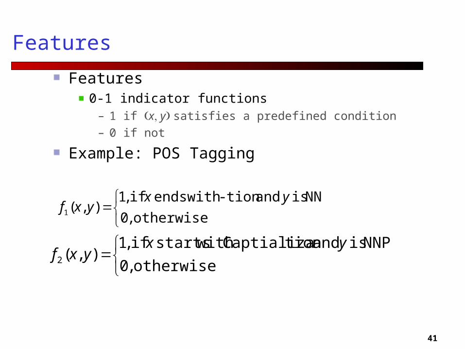
Features
Features0-1 indicator functions
– 1 if x y satisfies a predefined condition
– 0 if not
Example: POS Tagging
otherwise
NN is and tion- with ends if
,0
,1),(1
yxyxf
otherwise ,0
NNP is andtion Captializa with starts if ,1),(2
yxyxf
42
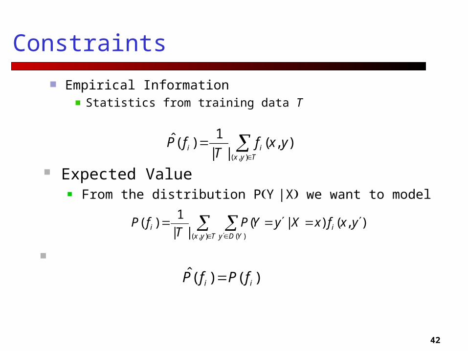
Constraints
Empirical InformationStatistics from training data T
Tyx
ii yxfT
fP),(
),(||
1)(ˆ
Constraints)()(ˆ
ii fPfP
Tyx YDy
ii yxfxXyYPT
fP),( )(
),()|(||
1)(
Expected Value From the distribution PY|X we want to model
43
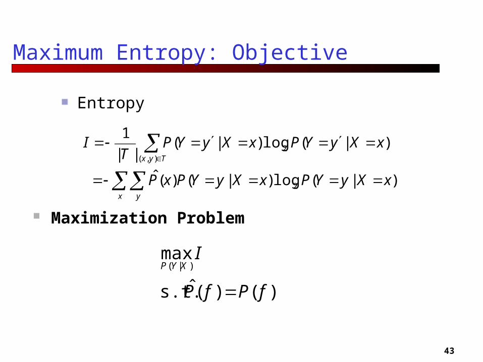
Maximum Entropy: Objective
Entropy
x y
Tyx
xXyYPxXyYPxP
xXyYPxXyYPT
I
)|(log)|()(ˆ
)|(log)|(||
1
2
),(2
)()(ˆ s.t.
max)|(
fPfP
IXYP
Maximization Problem
44
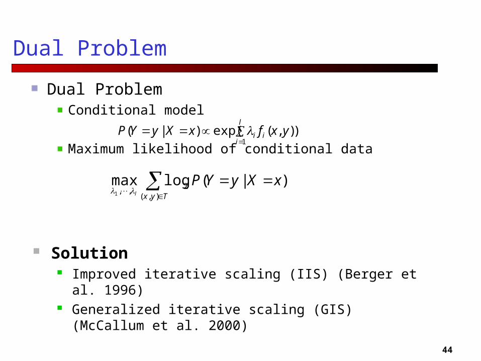
Dual Problem
Dual Problem Conditional model
Maximum likelihood of conditional data)),(exp()|(
1
l
iii yxfxXyYP
Solution Improved iterative scaling (IIS) (Berger et al. 1996) Generalized iterative scaling (GIS) (McCallum et al.
2000)
Tyx
xXyYPl ),(
2,,
)|(logmax1
45
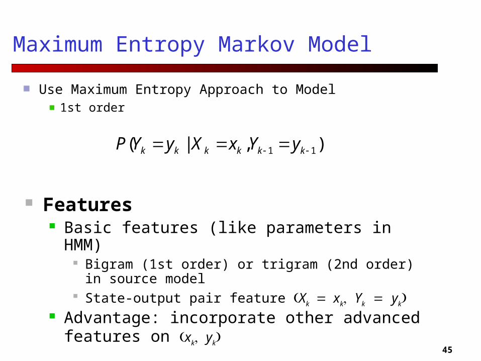
Maximum Entropy Markov Model
Use Maximum Entropy Approach to Model1st order
),|( 11 kkkkkk yYxXyYP
Features Basic features (like parameters in HMM)
Bigram (1st order) or trigram (2nd order) in source model
State-output pair feature Xkxk Yk yk Advantage: incorporate other advanced
features on xk yk
46
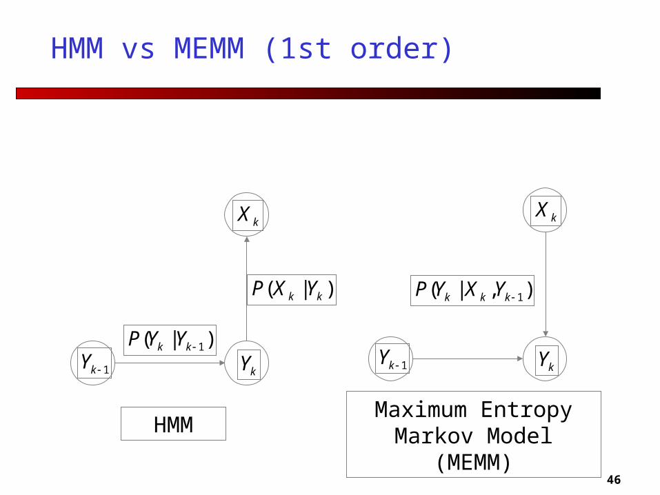
HMM vs MEMM (1st order)
kY1kY
kX
)|( 1kk YYP
)|( kk YXP
HMMMaximum Entropy
Markov Model (MEMM)
kY1kY
kX
),|( 1kkk YXYP
47
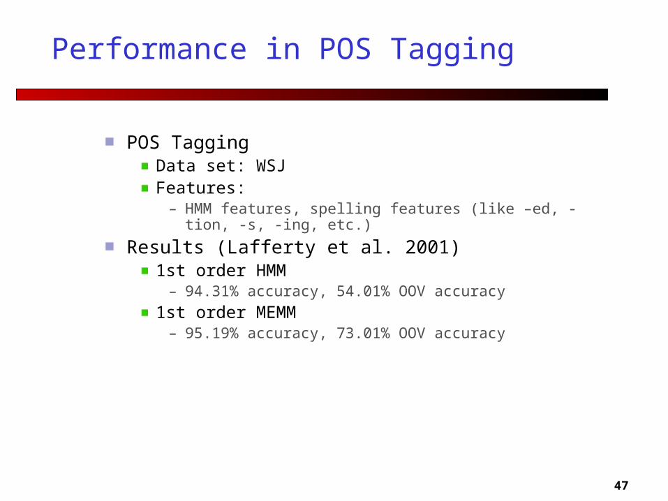
Performance in POS Tagging
POS TaggingData set: WSJFeatures:
– HMM features, spelling features (like –ed, -tion, -s, -ing, etc.)
Results (Lafferty et al. 2001)1st order HMM
– 94.31% accuracy, 54.01% OOV accuracy
1st order MEMM– 95.19% accuracy, 73.01% OOV accuracy
48
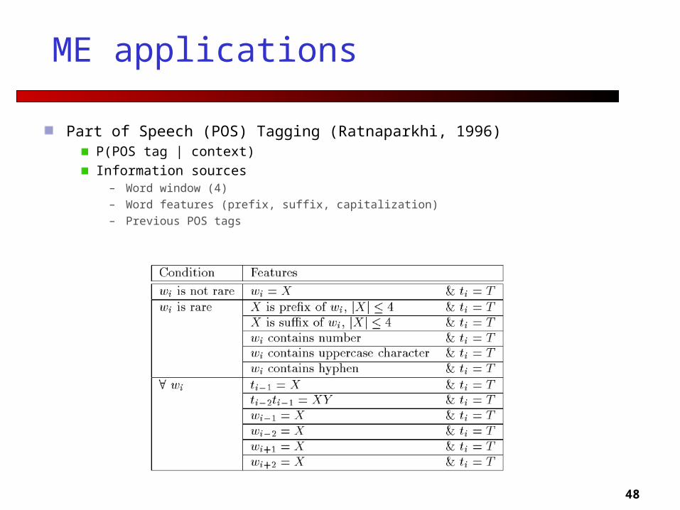
ME applications
Part of Speech (POS) Tagging (Ratnaparkhi, 1996)P(POS tag | context)
Information sources– Word window (4)– Word features (prefix, suffix, capitalization)– Previous POS tags
49
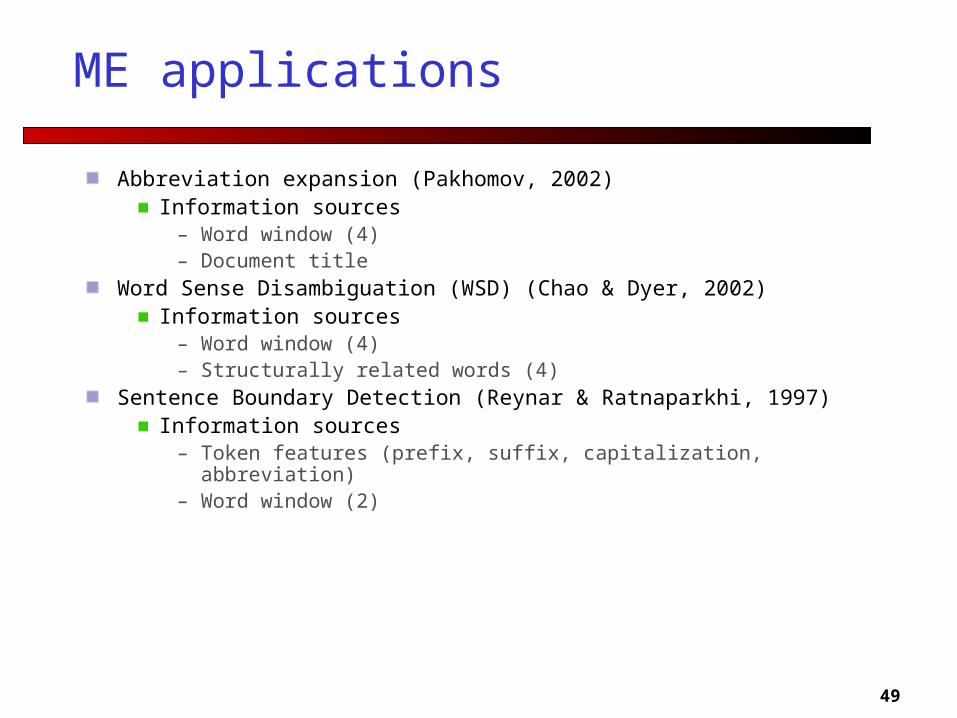
ME applications
Abbreviation expansion (Pakhomov, 2002)Information sources
– Word window (4)– Document title
Word Sense Disambiguation (WSD) (Chao & Dyer, 2002)Information sources
– Word window (4)– Structurally related words (4)
Sentence Boundary Detection (Reynar & Ratnaparkhi, 1997)Information sources
– Token features (prefix, suffix, capitalization, abbreviation)– Word window (2)
50
Solution
Global OptimizationOptimize parameters in a global model simultaneously, not in sub models separately
AlternativesConditional random fields
Application of perceptron algorithm
51
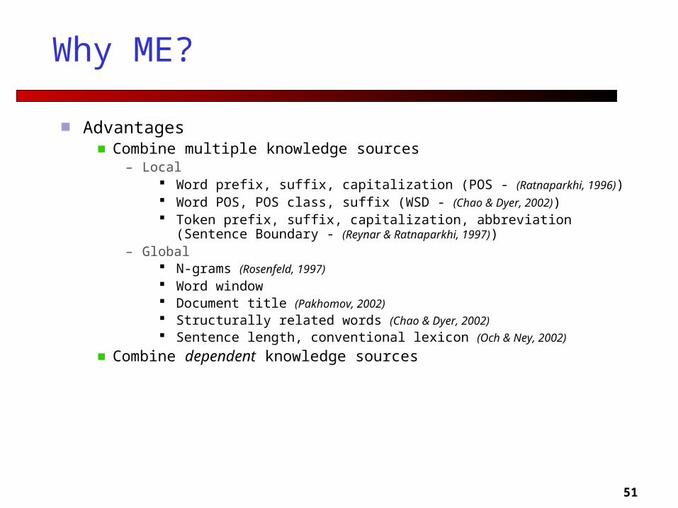
Why ME?
AdvantagesCombine multiple knowledge sources
– Local Word prefix, suffix, capitalization (POS - (Ratnaparkhi, 1996)) Word POS, POS class, suffix (WSD - (Chao & Dyer, 2002)) Token prefix, suffix, capitalization, abbreviation (Sentence Boundary -
(Reynar & Ratnaparkhi, 1997))– Global
N-grams (Rosenfeld, 1997) Word window Document title (Pakhomov, 2002) Structurally related words (Chao & Dyer, 2002) Sentence length, conventional lexicon (Och & Ney, 2002)
Combine dependent knowledge sources
52
Why ME?
AdvantagesAdd additional knowledge sources
Implicit smoothing
DisadvantagesComputational
– Expected value at each iteration
– Normalizing constant
Overfitting– Feature selection
Cutoffs Basic Feature Selection (Berger et al., 1996)
53
Conditional Models
Conditional probability P(label sequence y | observation sequence x) rather than joint probability P(y, x)
Specify the probability of possible label sequences given an observation sequence
Allow arbitrary, non-independent features on the observation sequence X
The probability of a transition between labels may depend on past and future observations
Relax strong independence assumptions in generative models
54
Discriminative ModelsMaximum Entropy Markov Models (MEMMs)
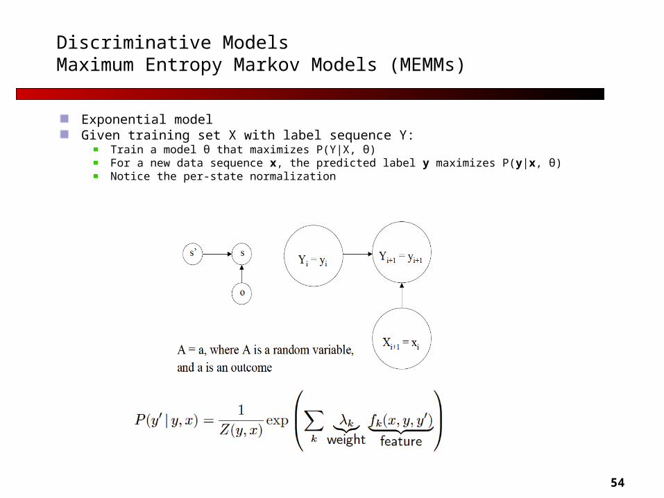
Exponential modelGiven training set X with label sequence Y:
Train a model θ that maximizes P(Y|X, θ)For a new data sequence x, the predicted label y maximizes P(y|x, θ)Notice the per-state normalization

55
MEMMs (cont’d)
MEMMs have all the advantages of Conditional Models
Per-state normalization: all the mass that arrives at a state must be distributed among the possible successor states (“conservation of score mass”)
Subject to Label Bias Problem
Bias toward states with fewer outgoing transitions
56
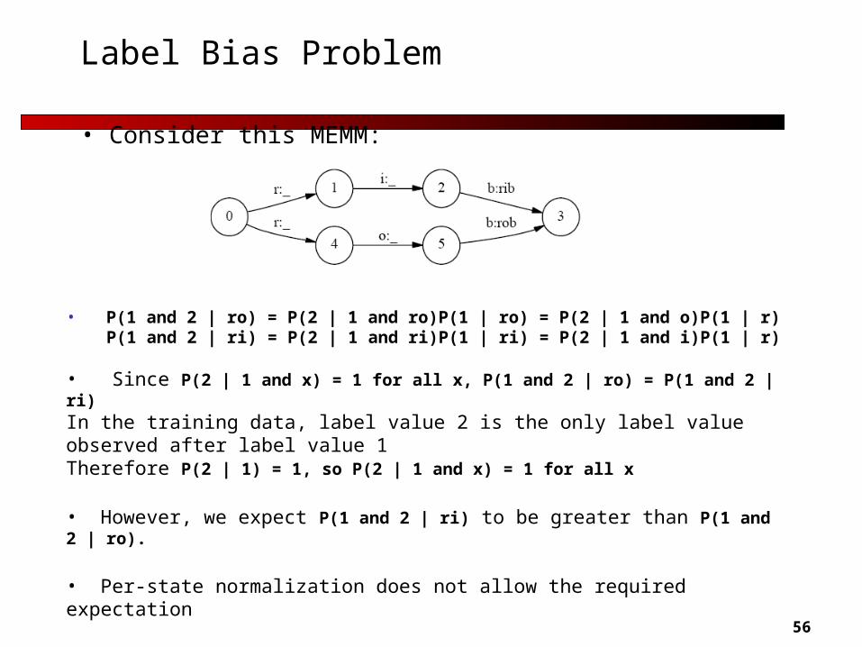
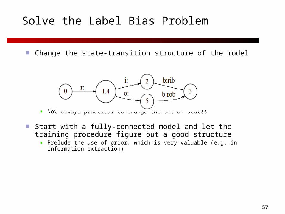
Label Bias Problem
• P(1 and 2 | ro) = P(2 | 1 and ro)P(1 | ro) = P(2 | 1 and o)P(1 | r) P(1 and 2 | ri) = P(2 | 1 and ri)P(1 | ri) = P(2 | 1 and i)P(1 | r)
• Since P(2 | 1 and x) = 1 for all x, P(1 and 2 | ro) = P(1 and 2 | ri)In the training data, label value 2 is the only label value observed after label value 1Therefore P(2 | 1) = 1, so P(2 | 1 and x) = 1 for all x
• However, we expect P(1 and 2 | ri) to be greater than P(1 and 2 | ro).
• Per-state normalization does not allow the required expectation
• Consider this MEMM:
57
Solve the Label Bias Problem
Change the state-transition structure of the model
Not always practical to change the set of states
Start with a fully-connected model and let the training procedure figure out a good structure
Prelude the use of prior, which is very valuable (e.g. in information extraction)

58
Random Field
59
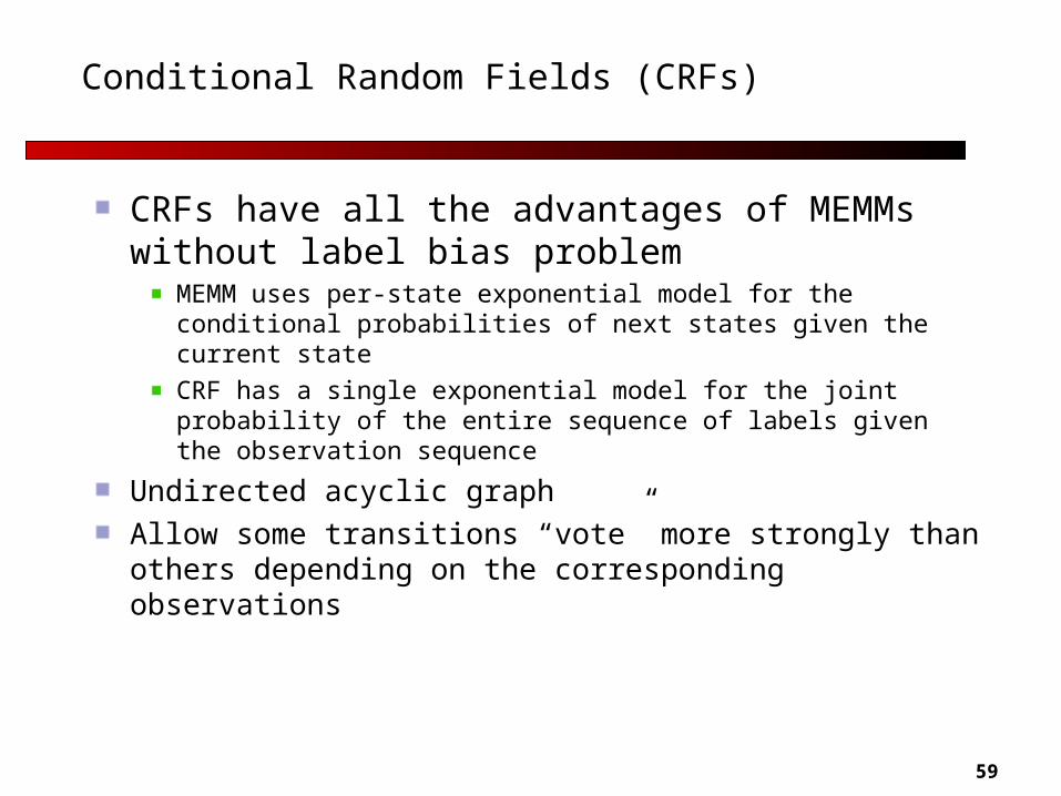
Conditional Random Fields (CRFs)
CRFs have all the advantages of MEMMs without label bias problem
MEMM uses per-state exponential model for the conditional probabilities of next states given the current state
CRF has a single exponential model for the joint probability of the entire sequence of labels given the observation sequence
Undirected acyclic graph
Allow some transitions “vote” more strongly than others depending on the corresponding observations
60
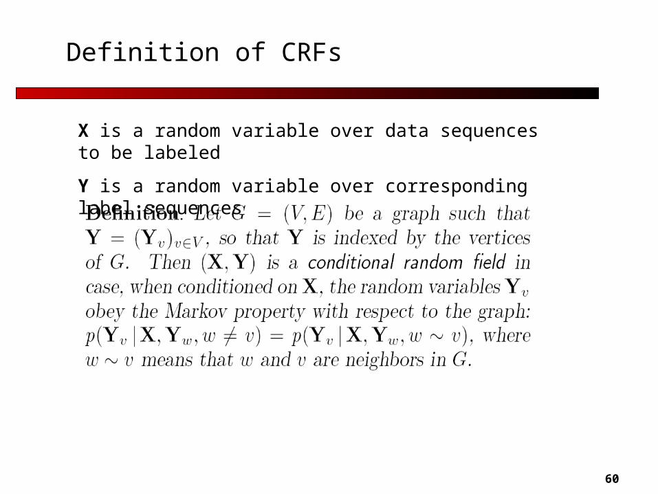
Definition of CRFs
X is a random variable over data sequences to be labeled
Y is a random variable over corresponding label sequences
61
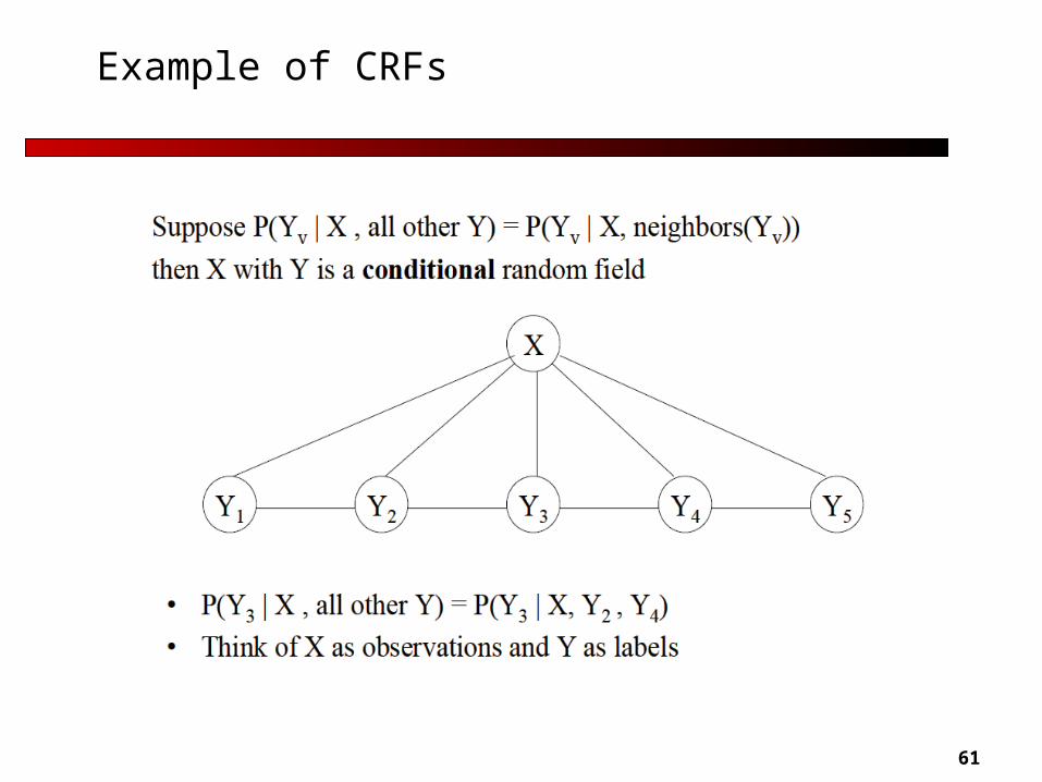
Example of CRFs
62
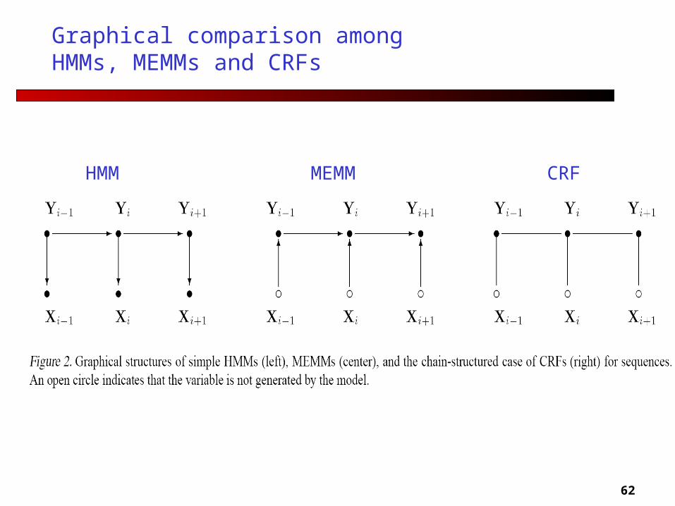
Graphical comparison among HMMs, MEMMs and CRFs
HMM MEMM CRF
63
Conditional Distribution
1 2 1 2( , , , ; , , , ); andn n k k
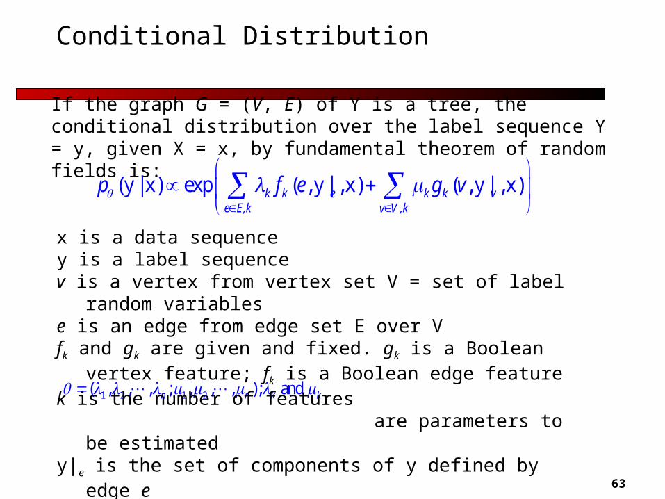
x is a data sequencey is a label sequence v is a vertex from vertex set V = set of label random variablese is an edge from edge set E over Vfk and gk are given and fixed. gk is a Boolean vertex feature; fk is a
Boolean edge featurek is the number of features
are parameters to be estimated
y|e is the set of components of y defined by edge ey|v is the set of components of y defined by vertex v
If the graph G = (V, E) of Y is a tree, the conditional distribution over the label sequence Y = y, given X = x, by fundamental theorem of random fields is:
(y | x) exp ( , y | , x) ( , y | , x)
k k e k k v
e E,k v V ,k
p f e g v
64
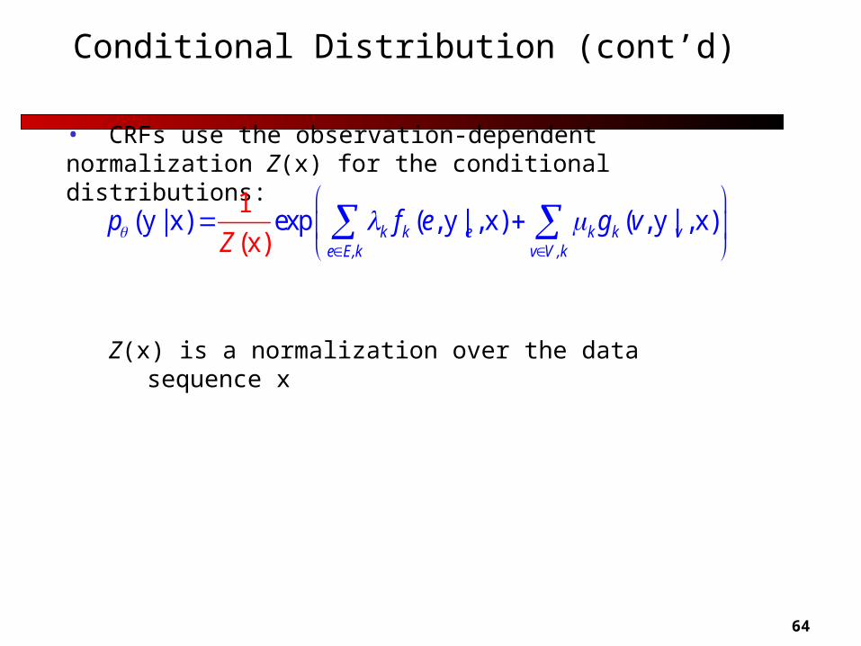
Conditional Distribution (cont’d)
• CRFs use the observation-dependent normalization Z(x) for the conditional distributions:
Z(x) is a normalization over the data sequence x
(y | x) exp ( , y | , x) ( , y |1
(x), x)
k k e k k v
e E,k v V ,k
p f e g vZ
65
Parameter Estimation for CRFs
The paper provided iterative scaling algorithms
It turns out to be very inefficient
Prof. Dietterich’s group applied Gradient Descendent Algorithm, which is quite efficient
66
Training of CRFs (From Prof. Dietterich)
log ( | )( , y | , x) ( , y | , x) log (x)
k k e k k ve E,k v V ,k
p y xf e g v Z
log ( | ) ( , y | , x) ( , y | , x) log (x)k k e k k ve E,k v V ,k
p y x f e g v Z
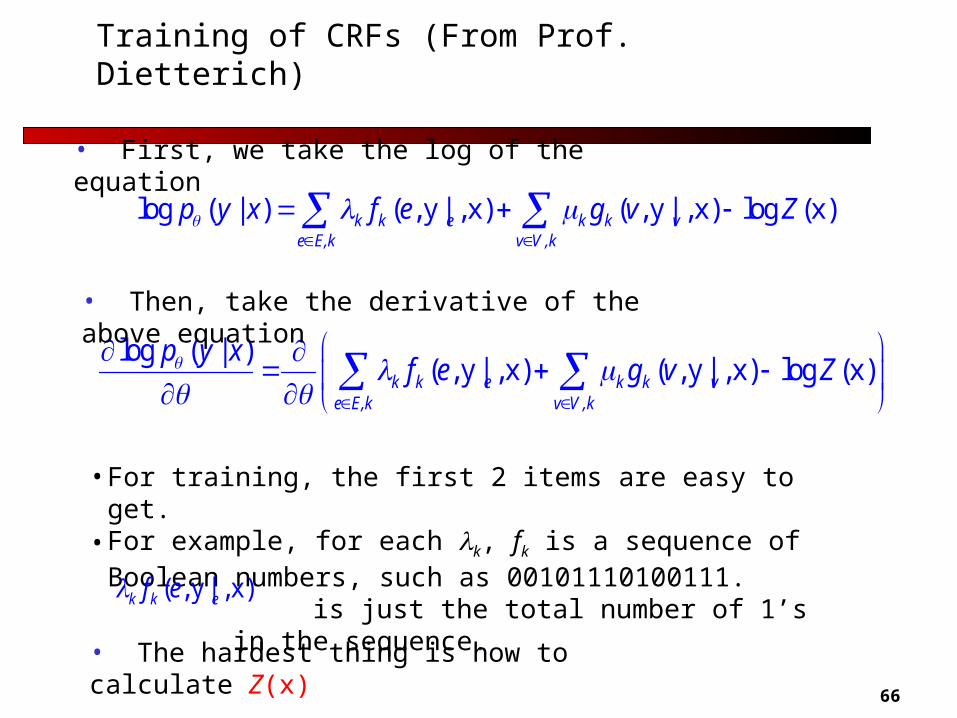
• First, we take the log of the equation
• Then, take the derivative of the above equation
• For training, the first 2 items are easy to get. • For example, for each k, fk is a sequence of Boolean numbers, such
as 00101110100111. is just the total number of 1’s in the sequence.( , y | , x)k k ef e
• The hardest thing is how to calculate Z(x)
67
Training of CRFs (From Prof. Dietterich) (cont’d)
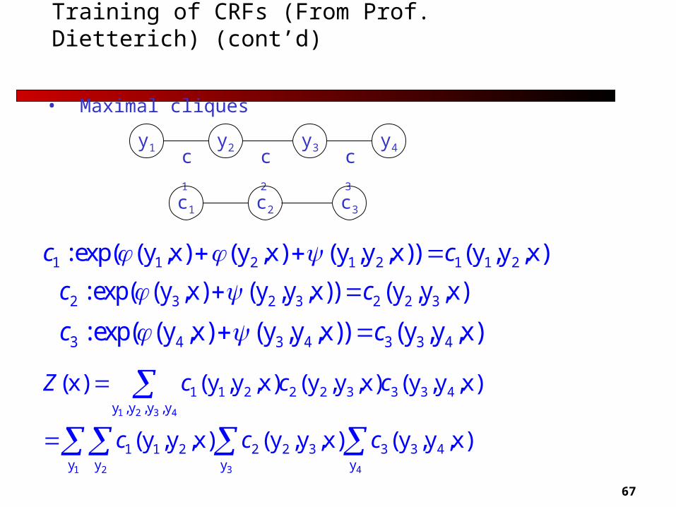
• Maximal cliques
y1 y2 y3 y4c1 c2 c3
c1 c2 c3
1 2 3 4
1 2 3 4
1 1 2 2 2 3 3 3 4y ,y ,y ,y
1 1 2 2 2 3 3 3 4y y y y
(x) (y ,y ,x) (y ,y ,x) (y ,y ,x)
(y ,y ,x) (y ,y ,x) (y ,y ,x)
Z c c c
c c c
3 4 3 4 3 3 4: exp( (y ,x) (y ,y ,x)) (y ,y ,x)c c
1 1 2 1 2 1 1 2: exp( (y ,x) (y ,x) (y ,y ,x)) (y ,y ,x)c c
2 3 2 3 2 2 3: exp( (y ,x) (y ,y ,x)) (y ,y ,x)c c

68
POS tagging Experiments
69
POS tagging Experiments (cont’d)
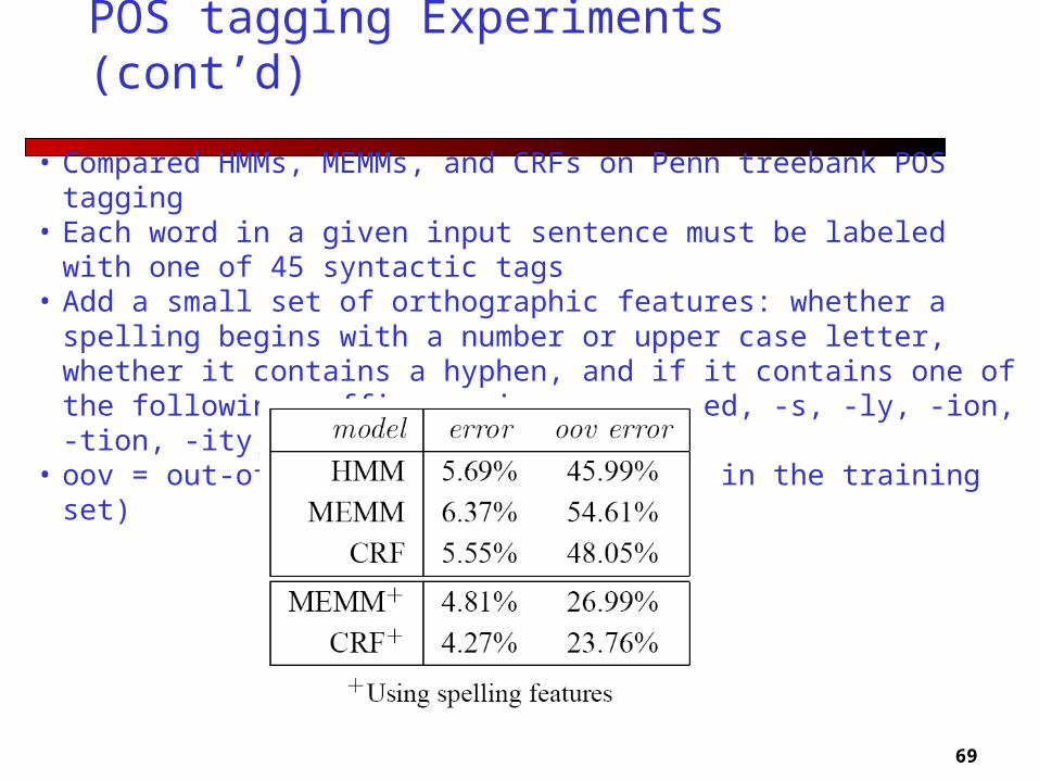
• Compared HMMs, MEMMs, and CRFs on Penn treebank POS tagging• Each word in a given input sentence must be labeled with one of 45 syntactic tags• Add a small set of orthographic features: whether a spelling begins with a number
or upper case letter, whether it contains a hyphen, and if it contains one of the following suffixes: -ing, -ogy, -ed, -s, -ly, -ion, -tion, -ity, -ies
• oov = out-of-vocabulary (not observed in the training set)
70
Summary
Discriminative models are prone to the label bias problem
CRFs provide the benefits of discriminative models
CRFs solve the label bias problem well, and demonstrate good performance