1-s2.0-S0143974X10002749-main

7/30/2019 1-s2.0-S0143974X10002749-main

http://slidepdf.com/reader/full/1-s20-s0143974x10002749-main 1/8

Journal of Constructional Steel Research 67 (2011) 585–592

Contents lists available at ScienceDirect

Journal of Constructional Steel Research

journal homepage: www.elsevier.com/locate/jcsr

Nonlinear inelastic analysis of space frames

Huu-Tai Thai, Seung-Eock Kim ∗

Department of Civil and Environmental Engineering, Sejong University, 98 Gunja Dong Gwangjin Gu, Seoul 143-747, Republic of Korea

a r t i c l e i n f o

Article history:

Received 20 September 2010

Accepted 4 December 2010

Keywords:

Nonlinear analysis

Stability function

Space frame

Geometric nonlinearity

Material nonlinearity

a b s t r a c t

In this paper, a fiber beam–column element which considers both geometric and material nonlinearitiesis presented. The geometric nonlinearities are captured using stability functions obtained from the

exact stability solution of a beam–column subjected to axial force and bending moments. The materialnonlinearities are included by tracing the uniaxial stress–strain relationship of each fiber on the crosssections. The nonlinear equilibrium equations are solved using an incremental iterative scheme based on

the generalized displacement control method. Usingonly one element per member in structure modeling,the nonlinearresponsespredictedby the proposed element compare wellwith thosegiven by commercial

finite element packages and other available results. Numerical examples are presented to verify theaccuracy and efficiency of the proposed element.

© 2010 Elsevier Ltd. All rights reserved.

1. Introduction

In the past few decades, there have been numerous studiesto improve the accuracy of the beam–column element for thenonlinear analysis of steel frames. In general, the nonlinear

response of steel frames can be predicted by using either thefinite element method or the beam–column approach. The finiteelement approach is often based on a stiffness or displacementformulation in which cubic and linear interpolation functions areused forthe transverse andaxialdisplacements, respectively[1–5].Since this method is based commonly on an assumed cubicpolynomial variation of transverse displacement alongthe elementlength, it is unable to capture accurately the effect of axial forceacting through the lateral displacement of the element (P –δeffect) when one element per member is used [6]. Hence, itoverestimates the strength of a member under significant axialforce. Although the accuracy of this method can be improvedby using several elements per member in the modeling, it isgenerally recognized to be computationally intensive because of

a very refined discretisation of the structures. The beam–columnapproach is based on the stabilityfunctionswhich arederived fromthe exact stability function of a beam–column subjected to axialforce and bending moments [7–12]. This approach can captureaccurately the P –δ effect of a beam–column member by using onlyone or two elements per member in the modeling, hence, to savecomputational time.

In parallel with the above developments, different beam–column models have been proposed to represent inelastic material

∗ Corresponding author. Tel.: +82 2 3408 3291; fax: +82 2 3408 3332.

E-mail addresses: [email protected](H.-T. Thai), [email protected](S.-E. Kim).

behavior. These models can be grouped into two categories:

lumped plasticity [9,10,13] model and distributed plasticity model

[5,14–18]. In the lumped plasticity model, the inelastic behavior

of material is assumed to be concentrated at point hinges that are

usually located at the ends of the member. The force–deformation

relation at these hinges is based on force resultants. The advantage

of this model is that it is simple in formulation as well as

implementation. However, the disadvantage of this model is that

theforce–deformation relation at thehingesis notalways available

and accurate for every section. In the distributed plasticity model,

the inelastic behavior of material is distributed along the member

length since the element behavior is monitored through numerical

integration of constitutive behavior at a finite number of control

sections. The nonlinear constitutive behavior at these sections

is derived using one of the following methods: (1) moment–

curvature relations; (2) force and deformation resultants; and

(3) uniaxial stress–strain relations of fibers on the cross sections.

Although fiber model is the most computationallyintensiveamong

others, it represents the inelastic behavior of material more

accurately and rationally than concentrated plasticity model.

This paper proposes a fiber beam–column element for the

nonlinear inelastic analysis of space steel frames. The spread of

plasticity over the cross section and along the member length is

captured by tracing the uniaxial stress–strain relations of each

fiber on the cross sections located at the selected integration

points along the member length. The Gauss–Lobatto integration

rule is adopted herein for evaluating numerically element stiffness

matrix instead of the classical Gauss integration rule because

it always includes the end sections of the integration field.

Since inelastic behavior in beam elements often concentrates at

the ends of the member, monitoring the end sections of the

element results in improved accuracy and numerical stability [19].

0143-974X/$ – see front matter © 2010 Elsevier Ltd. All rights reserved.doi:10.1016/j.jcsr.2010.12.003

http://dx.doi.org/10.1016/j.jcsr.2010.12.003

http://www.elsevier.com/locate/jcsr


mailto:[email protected]









7/30/2019 1-s2.0-S0143974X10002749-main


586 H.-T. Thai, S.-E. Kim / Journal of Constructional Steel Research 67 (2011) 585–592

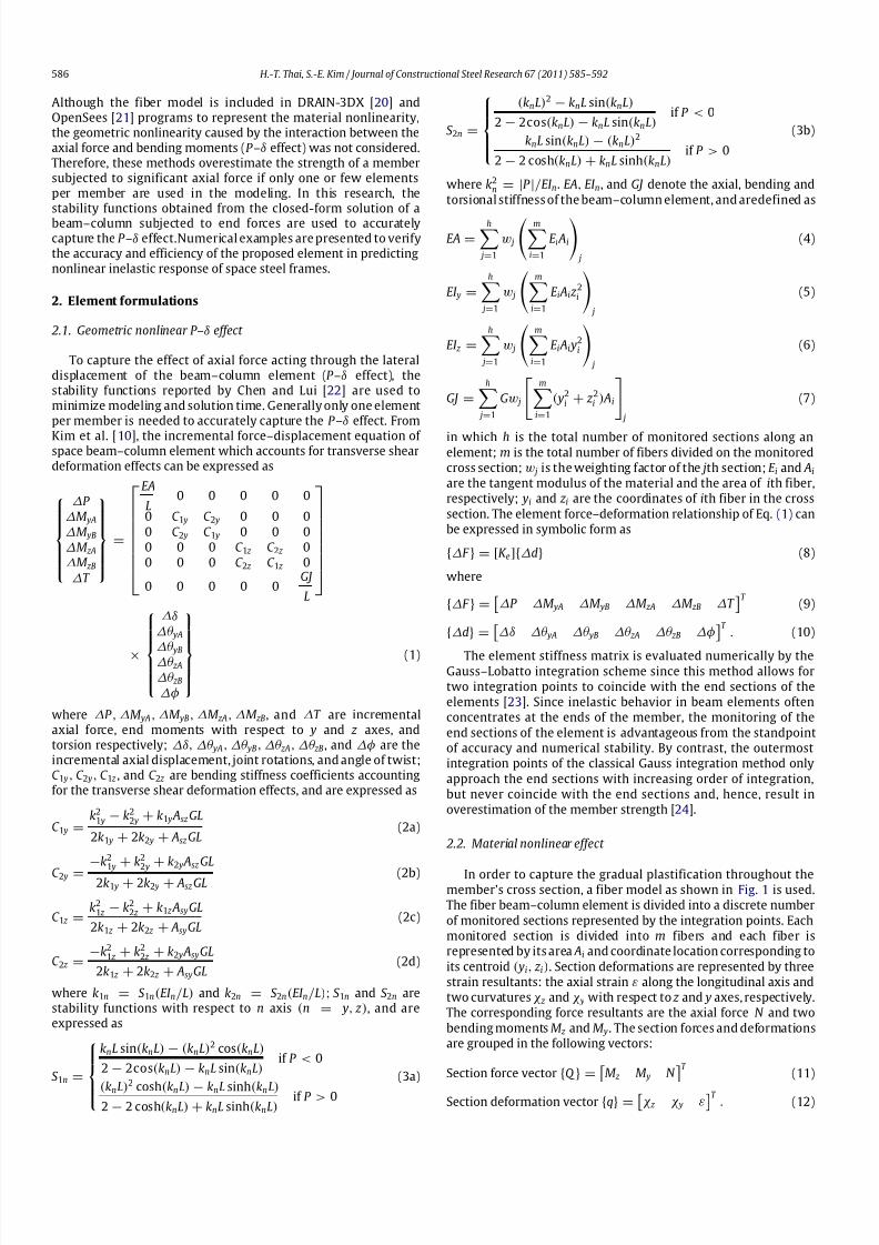
Although the fiber model is included in DRAIN-3DX [20] andOpenSees [21] programs to represent the material nonlinearity,the geometric nonlinearity caused by the interaction between theaxial force and bending moments (P –δ effect) was not considered.Therefore, these methods overestimate the strength of a membersubjected to significant axial force if only one or few elementsper member are used in the modeling. In this research, thestability functions obtained from the closed-form solution of abeam–column subjected to end forces are used to accuratelycapture the P –δ effect.Numerical examples are presented to verifythe accuracy and efficiency of the proposed element in predictingnonlinear inelastic response of space steel frames.

2. Element formulations

2.1. Geometric nonlinear P–δ effect

To capture the effect of axial force acting through the lateraldisplacement of the beam–column element (P –δ effect), thestability functions reported by Chen and Lui [22] are used tominimize modeling and solution time. Generally only one elementper member is needed to accurately capture the P –δ effect. From

Kim et al. [10], the incremental force–displacement equation of space beam–column element which accounts for transverse sheardeformation effects can be expressed as

∆P

∆M yA

∆M yB

∆M zA

∆M zB

∆T

=

EA

L0 0 0 0 0

0 C 1 y C 2 y 0 0 0

0 C 2 y C 1 y 0 0 00 0 0 C 1 z C 2 z 00 0 0 C 2 z C 1 z 0

0 0 0 0 0GJ

L

×

∆δ∆θ yA

∆θ yB∆θ zA

∆θ zB

∆φ

(1)

where ∆P , ∆M yA, ∆M yB, ∆M zA, ∆M zB, and ∆T are incrementalaxial force, end moments with respect to y and z axes, andtorsion respectively; ∆δ, ∆θ yA, ∆θ yB, ∆θ zA, ∆θ zB, and ∆φ are theincremental axial displacement, joint rotations, and angle of twist;C 1 y, C 2 y, C 1 z , and C 2 z are bending stiffness coefficients accountingfor the transverse shear deformation effects, and are expressed as

C 1 y =k2

1 y − k22 y + k1 y Asz GL

2k1 y + 2k2 y + Asz GL(2a)

C 2 y =

−k21 y + k2

2 y + k2 y Asz GL

2k1 y + 2k2 y + Asz GL (2b)

C 1 z =k2

1 z − k22 z + k1 z AsyGL

2k1 z + 2k2 z + AsyGL(2c)

C 2 z =−k2

1 z + k22 z + k2 y AsyGL

2k1 z + 2k2 z + AsyGL(2d)

where k1n = S 1n(EI n/L) and k2n = S 2n(EI n/L); S 1n and S 2n arestability functions with respect to n axis (n = y, z ), and areexpressed as

S 1n =

knL sin(knL) − (knL)2 cos(knL)

2 − 2cos(knL) − knL sin(knL)if P < 0

(knL)2

cosh(knL) − knL sinh(knL)2 − 2 cosh(knL) + knL sinh(knL)

if P > 0

(3a)

S 2n =

(knL)2 − knL sin(knL)

2 − 2cos(knL) − knL sin(knL)if P < 0

knL sin(knL) − (knL)2

2 − 2 cosh(knL) + knL sinh(knL)if P > 0

(3b)

where k2n = |P |/EI n. EA, EI n, and GJ denote the axial, bending and

torsional stiffness of the beam–column element, and aredefined as

EA =

h− j=1

w j

m−

i=1

E i Ai

j

(4)

EI y =

h− j=1

w j

m−

i=1

E i Ai z 2i

j

(5)

EI z =

h− j=1

w j

m−

i=1

E i Ai y2i

j

(6)

GJ =

h− j=1

Gw j

m−

i=1

( y2i + z 2i ) Ai

j

(7)

in which h is the total number of monitored sections along anelement; m is the total number of fibers divided on the monitoredcross section; w j is the weighting factor of the jth section; E i and Ai

are the tangent modulus of the material and the area of ith fiber,respectively; yi and z i are the coordinates of ith fiber in the cross

section. The element force–deformation relationship of Eq. (1) canbe expressed in symbolic form as

{∆F } = [K e]{∆d} (8)

where

{∆F } =

∆P ∆M yA ∆M yB ∆M zA ∆M zB ∆T T

(9)

{∆d} = ∆δ ∆θ yA ∆θ yB ∆θ zA ∆θ zB ∆φT

. (10)

The element stiffness matrix is evaluated numerically by theGauss–Lobatto integration scheme since this method allows fortwo integration points to coincide with the end sections of theelements [23]. Since inelastic behavior in beam elements oftenconcentrates at the ends of the member, the monitoring of the

end sections of the element is advantageous from the standpointof accuracy and numerical stability. By contrast, the outermostintegration points of the classical Gauss integration method only

approach the end sections with increasing order of integration,but never coincide with the end sections and, hence, result inoverestimation of the member strength [24].

2.2. Material nonlinear effect

In order to capture the gradual plastification throughout themember’s cross section, a fiber model as shown in Fig. 1 is used.The fiber beam–column element is divided into a discrete number

of monitored sections represented by the integration points. Eachmonitored section is divided into m fibers and each fiber isrepresented by its area Ai and coordinate location corresponding to

its centroid ( yi, z i). Section deformations are represented by threestrain resultants: the axial strain ε along the longitudinal axis andtwo curvatures χ z and χ y with respect to z and y axes, respectively.The corresponding force resultants are the axial force N and two

bending moments M z and M y. The section forces and deformationsare grouped in the following vectors:

Section force vector {Q } = M z M y N T

(11)

Section deformation vector {q} =

χ z χ y εT

. (12)

7/30/2019 1-s2.0-S0143974X10002749-main


H.-T. Thai, S.-E. Kim / Journal of Constructional Steel Research 67 (2011) 585–592 587

Fig. 1. Fiber concept.

The incremental section force vector at each integration points is

determined based on the incremental element force vector {∆F }as

{∆Q } = [B( x)] {∆F } (13)

where [B( x)] is the force interpolation function matrix given as

[B( x)] =

−δ y( x) 0 0 ( x/L − 1) x/L 0−δ z ( x) ( x/L − 1) x/L 0 0 0

1 0 0 0 0 0

(14)

where δ y( x) and δ z ( x) are the lateral displacements for the local y

and z axes, respectively. Since the curvature can be approximated

by thesecondderivative of the lateral displacement, δ y( x) and δ z ( x)

are obtained from solving the differential equations as [22]

δ y( x) = −M zA

EI z k2

z

[sin(k z x)

tan(k z L)− cos(k z x) −

x

L+ 1

]

−M zB

EI z k2 z

[sin(k z x)

sin(k z L)−

x

L

](15)

δ z ( x) =M yA

EI yk2 y

[sin(k y x)

tan(k yL)− cos(k y x) −

x

L+ 1

]

+M yB

EI yk2 y

[sin(k y x)

sin(k yL)−

x

L

]. (16)

The section deformation vector is determined based on the section

force vector as

{∆q} = [ksec]−1{∆Q } (17)

where [ksec] is the section stiffness matrix given as

[ksec] =

m−i=1

E i Ai y2i

m−i=1

E i Ai yi z i

m−i=1

E i Ai(− yi)

m−i=1

E i Ai yi z i

m−i=1

E i Ai z 2i

m−i=1

E i Ai z i

m−i=1

E i Ai(− yi)

m−i=1

E i Ai z i

m−i=1

E i Ai

. (18)

Followingthe hypothesis that plane sections remainplane andnor-mal to the longitudinal axis, the incremental uniaxial fiber strain

vector is computed based on the incremental section deformationvector as

{∆e} = [l]{∆q} (19)

where [l] is the linear geometric matrix given as follows

[l] =

− y1 z 1 1− y2 z 2 1

· · · · · · · · ·− ym z m 1

. (20)

Once the incremental fiber strain is evaluated, the incrementalfiber stress is computed based on the stress–strain relationship of material model. The tangent modulus of each fiber is updated fromthe incremental fiber stress and incremental fiber strain as

E i =∆σ i

∆ei

. (21)

Eq. (21) leads to updating of the element stiffness matrix [K e] inEq. (8) and section stiffness matrix [ksec] in Eq. (18) during theiteration process. Based on the new tangent modulus of Eq. (21),the location of the section centroid is also updated during theincremental load steps to take into account the distribution of section plasticity. The section resisting forces are computed by

summation of the axial force and biaxial bending moment contri-butions of all fibers as

{Q R} =

M z

M yN

=

m−i=1

σ i Ai(− yi)

m−i=1

σ i Ai z i

m−i=1

σ i Ai

. (22)

2.3. Element stiffness matrix accounting for P –∆ effect

The P –∆ effect is the effect of axial force P acting through the

relative transverse displacement of the member ends ∆. This effectcan be considered by using the geometric stiffness matrix [K g ] as

[K g ]12×12 =

[[K s] −[K s]

−[K s]T [K s]

](23)

where

[K s] =

0 a −b 0 0 0a c 0 0 0 0

−b 0 c 0 0 00 0 0 0 0 00 0 0 0 0 00 0 0 0 0 0

(24)

and

a = M zA + M zB

L2, b = M yA + M yB

L2, c = P

L. (25)

The displacement of a beam–column element can be decomposedinto two parts: the element deformation and rigid displacement.The element deformation increment {∆d} in Eq. (10) can beobtained from the element displacement increment {∆D} as

{∆d} = [T ]6×12{∆D} (26)

where

[T ]6×12

=

−1 0 0 0 0 0 1 0 0 0 0 0

0 0 −1/L 0 1 0 0 0 1/L 0 0 0

0 0 −1/L 0 0 0 0 0 1/L 0 1 0

0 1/L 0 0 0 1 0 −1/L 0 0 0 0

0 1/L 0 0 0 0 0 −1/L 0 0 0 10 0 0 1 0 0 0 0 0 −1 0 0

. (27)

7/30/2019 1-s2.0-S0143974X10002749-main



Thetangent stiffnessmatrix of a beam–column element is obtained

as follows

[K ]12×12 = [T ]T 6×12[K e]6×6[T ]6×12 + [K g ]12×12. (28)

3. Nonlinear solution procedure

This section presents a numerical method for solving thenonlinear equations. Among several numerical methods, the

GDC method proposed by Yang and Shieh [25] appears to beone of the most robust and effective methods for solving thenonlinear problems with multiple critical points because of itsgeneral numerical stability and efficiency. The incremental form

of equilibrium equation can be rewritten for the jth iteration of theith incremental step as

[K i j−1]{∆Di j} = λi

j{P̂ } + {Ri j−1} (29)

where [K i j−1] is the tangent stiffness matrix, {∆Di j} is the

displacement increment vector, {P̂ } is the reference load vector,{Ri

j−1} is the unbalanced force vector, and λi j is the load increment

parameter.

Eq. (29) can be decomposed into the following equations

[K i j−1]{∆D̂i j} = {P̂ } (30)

[K i j−1]{∆D̄i j} = {Ri

j−1} (31)

{∆Di j} = λi

j{∆D̂i j} + {∆D̄i

j}. (32)

The load increment parameter λi j is unknown. It is determinedfrom

a constraint condition. For the first iterative step ( j = 1), the loadincrement parameter λi

j is determined based on the Generalized

Stiffness Parameter (GSP ) as

λi1 = λ1

1

|GSP | (33)

where λ11 is an initial value of a load increment parameter, and the

GSP is defined as

GSP ={∆D̂1

1}T {∆D̂11}

{∆D̂i−11 }T {∆D̂i

1}. (34)

For the following iteration ( j ≥ 2), the load increment parameterλi

j is computed as

λi j = −

{∆D̂i−11 }T {∆D̄i

j}

{∆D̂i−11 }T {∆D̂i

j}(35)

where {∆D̂i−11 } is the displacement increment generated by the

reference load {P̂ } at the first iteration of the previous (i − 1)

incremental step, and {∆D̂i j} and {∆D̄i

j} denote the displacement

increments generated by the reference load and unbalanced forcevectors, respectively, at the jth iterationof the ith incremental step,

as defined in Eqs. (30) and (31).The following is a step-by-step summary of solution algorithm

focused on the element state determination process of a singleiteration.

1. Solve the global equation and update the element displace-ment increment {∆D}.

2. Compute the element deformation increment {∆d} using

Eq. (26).3. Compute the element force increment {∆F } using Eq. (8) based

on the element stiffness matrix [K e]6×6 of the previous step.4. Compute the section force increment {∆Q } using Eq. (13).5. Compute the section stiffness {ksec} using Eq. (18).

6. Compute the section deformation increment {∆q} usingEq. (17).

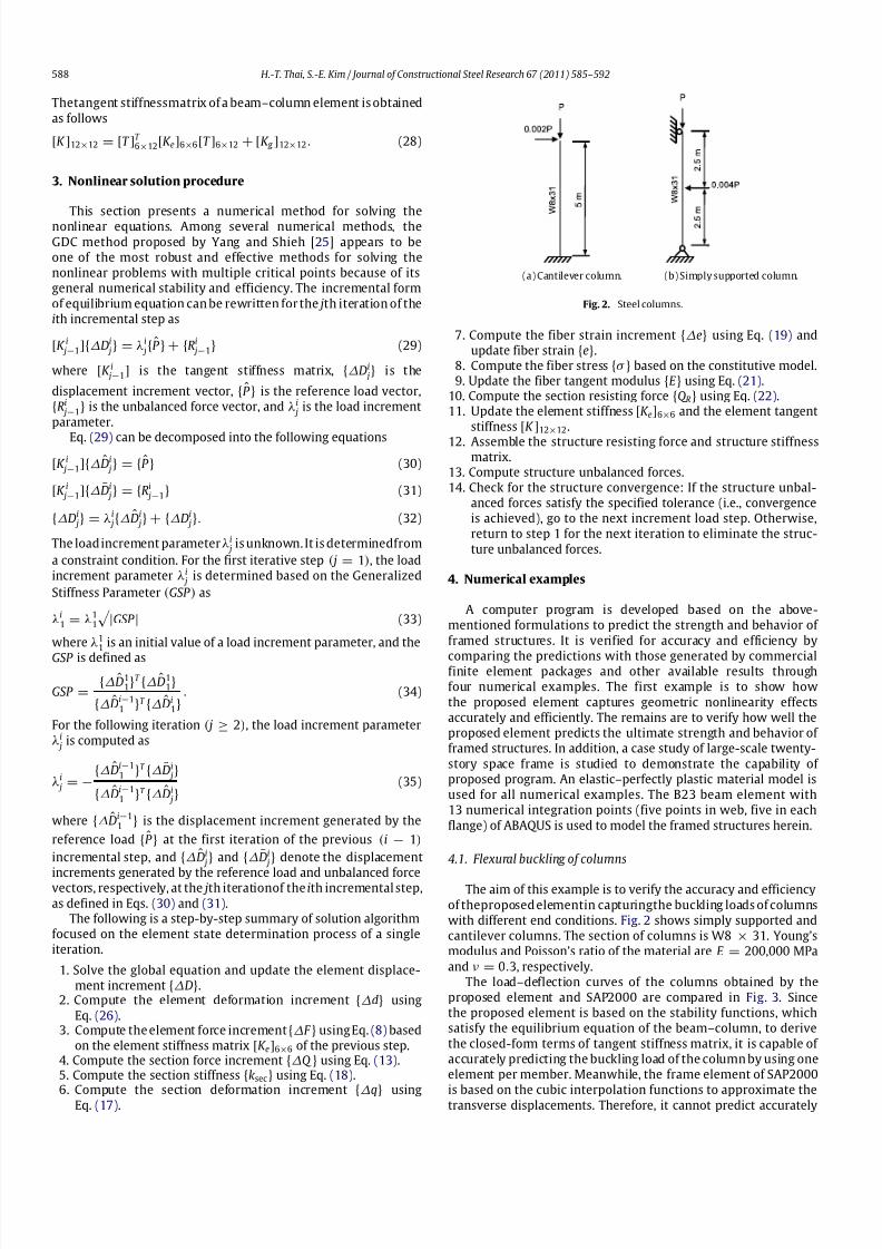
(a) Cantilever column. (b) Simply supported column.

Fig. 2. Steel columns.

7. Compute the fiber strain increment {∆e} using Eq. (19) andupdate fiber strain {e}.

8. Compute the fiber stress {σ } based on the constitutive model.9. Update the fiber tangent modulus {E } using Eq. (21).

10. Compute the section resisting force {Q R} using Eq. (22).11. Update the element stiffness [K e]6×6 and the element tangent

stiffness [K ]12×12.

12. Assemble the structure resisting force and structure stiffnessmatrix.

13. Compute structure unbalanced forces.14. Check for the structure convergence: If the structure unbal-

anced forces satisfy the specified tolerance (i.e., convergenceis achieved), go to the next increment load step. Otherwise,return to step 1 for the next iteration to eliminate the struc-

ture unbalanced forces.

4. Numerical examples

A computer program is developed based on the above-mentioned formulations to predict the strength and behavior of

framed structures. It is verified for accuracy and efficiency by

comparing the predictions with those generated by commercialfinite element packages and other available results throughfour numerical examples. The first example is to show how

the proposed element captures geometric nonlinearity effectsaccurately and efficiently. The remains are to verify how well theproposed element predicts the ultimate strength and behavior of framed structures. In addition, a case study of large-scale twenty-

story space frame is studied to demonstrate the capability of proposed program. An elastic–perfectly plastic material model isused for all numerical examples. The B23 beam element with13 numerical integration points (five points in web, five in each

flange) of ABAQUS is used to model the framed structures herein.

4.1. Flexural buckling of columns

The aim of this example is to verify the accuracy and efficiency

of theproposed elementin capturingthe buckling loads of columnswith different end conditions. Fig. 2 shows simply supported andcantilever columns. The section of columns is W8 × 31. Young’smodulus and Poisson’s ratio of the material are E = 200,000 MPa

and ν = 0.3, respectively.The load–deflection curves of the columns obtained by the

proposed element and SAP2000 are compared in Fig. 3. Sincethe proposed element is based on the stability functions, whichsatisfy the equilibrium equation of the beam–column, to derive

the closed-form terms of tangent stiffness matrix, it is capable of accurately predicting the buckling load of the column by using oneelement per member. Meanwhile, the frame element of SAP2000

is based on the cubic interpolation functions to approximate thetransverse displacements. Therefore, it cannot predict accurately

7/30/2019 1-s2.0-S0143974X10002749-main


H.-T. Thai, S.-E. Kim / Journal of Constructional Steel Research 67 (2011) 585–592 589

(a) Cantilever column. (b) Simply supported column.

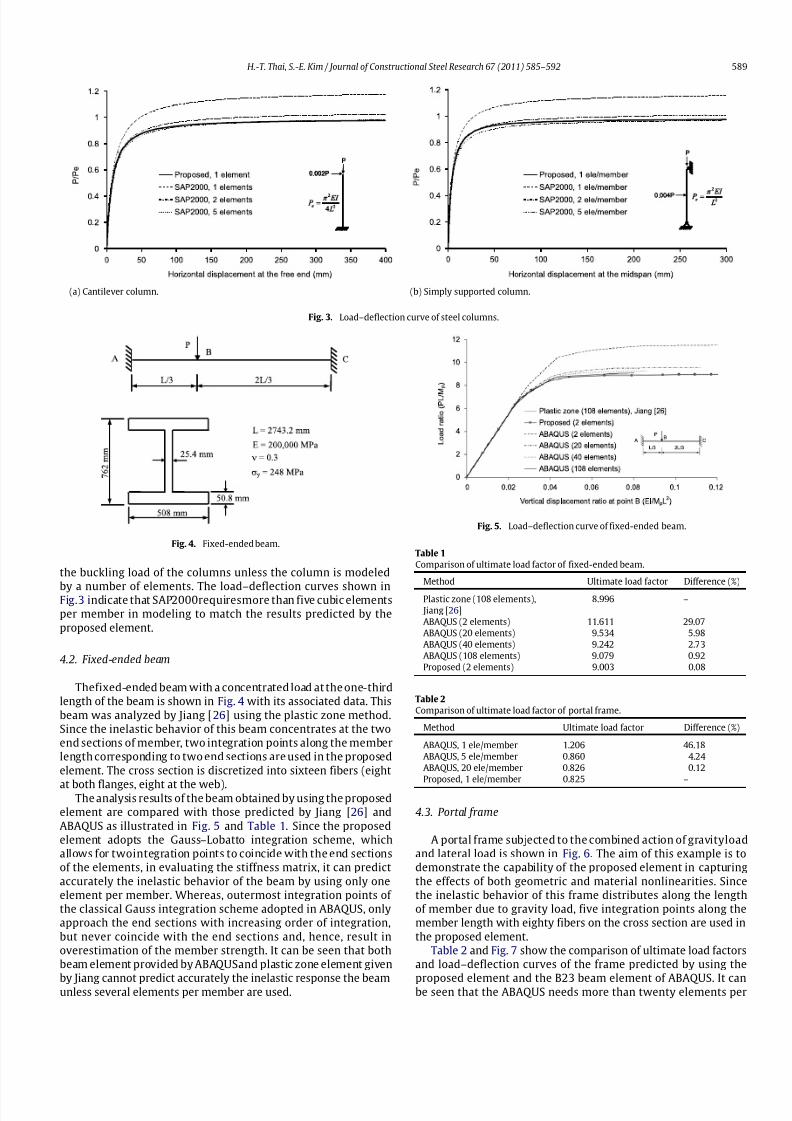
Fig. 3. Load–deflection curve of steel columns.

Fig. 4. Fixed-ended beam.

the buckling load of the columns unless the column is modeled

by a number of elements. The load–deflection curves shown inFig.3 indicate that SAP2000requiresmore than five cubic elementsper member in modeling to match the results predicted by the

proposed element.

4.2. Fixed-ended beam

Thefixed-ended beam with a concentrated load at the one-thirdlength of the beam is shown in Fig. 4 with its associated data. This

beam was analyzed by Jiang [26] using the plastic zone method.Since the inelastic behavior of this beam concentrates at the twoend sections of member, two integration points along the memberlength corresponding to two end sections are used in the proposed

element. The cross section is discretized into sixteen fibers (eight

at both flanges, eight at the web).The analysis results of the beam obtained by using the proposed

element are compared with those predicted by Jiang [26] and

ABAQUS as illustrated in Fig. 5 and Table 1. Since the proposedelement adopts the Gauss–Lobatto integration scheme, whichallows for twointegration points to coincide with the end sectionsof the elements, in evaluating the stiffness matrix, it can predict

accurately the inelastic behavior of the beam by using only oneelement per member. Whereas, outermost integration points of the classical Gauss integration scheme adopted in ABAQUS, onlyapproach the end sections with increasing order of integration,

but never coincide with the end sections and, hence, result inoverestimation of the member strength. It can be seen that bothbeam element provided by ABAQUSand plastic zone element given

by Jiang cannot predict accurately the inelastic response the beamunless several elements per member are used.

Fig. 5. Load–deflection curve of fixed-ended beam.

Table 1

Comparison of ultimate load factor of fixed-ended beam.

Method Ultimate load factor Difference (%)

Plastic zone (108 elements),

Jiang [26]

8.996 –

ABAQUS (2 elements) 11.611 29.07




Proposed (2 elements) 9.003 0.08

Table 2

Comparison of ultimate load factor of portal frame.

Method Ultimate load factor Difference (%)

ABAQUS, 1 ele/member 1.206 46.18



Proposed, 1 ele/member 0.825 –

4.3. Portal frame

A portal frame subjected to the combined action of gravityloadand lateral load is shown in Fig. 6. The aim of this example is todemonstrate the capability of the proposed element in capturing

the effects of both geometric and material nonlinearities. Sincethe inelastic behavior of this frame distributes along the lengthof member due to gravity load, five integration points along themember length with eighty fibers on the cross section are used in

the proposed element.Table 2 and Fig. 7 show the comparison of ultimate load factors

and load–deflection curves of the frame predicted by using the

proposed element and the B23 beam element of ABAQUS. It canbe seen that the ABAQUS needs more than twenty elements per

7/30/2019 1-s2.0-S0143974X10002749-main



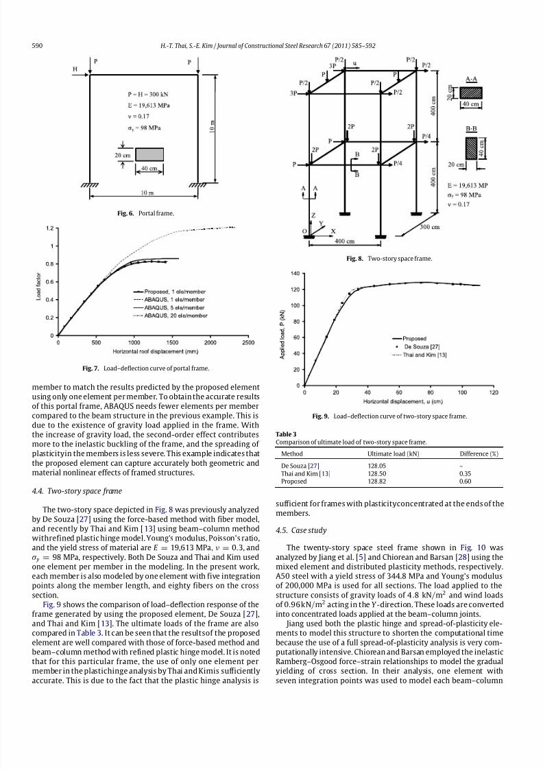
Fig. 6. Portal frame.

Fig. 7. Load–deflection curve of portal frame.

member to match the results predicted by the proposed elementusing only one element per member. To obtain the accurate results

of this portal frame, ABAQUS needs fewer elements per membercompared to the beam structure in the previous example. This is

due to the existence of gravity load applied in the frame. Withthe increase of gravity load, the second-order effect contributesmore to the inelastic buckling of the frame, and the spreading of plasticityin the members is less severe. This example indicates that

the proposed element can capture accurately both geometric andmaterial nonlinear effects of framed structures.

4.4. Two-story space frame

The two-story space depicted in Fig. 8 was previously analyzed

by De Souza [27] using the force-based method with fiber model,and recently by Thai and Kim [13] using beam–column method

withrefined plastic hinge model. Young’s modulus, Poisson’s ratio,and the yield stress of material are E = 19,613 MPa, ν = 0.3, andσ y = 98 MPa, respectively. Both De Souza and Thai and Kim usedone element per member in the modeling. In the present work,each member is also modeled by one element with five integrationpoints along the member length, and eighty fibers on the cross

section.Fig. 9 shows the comparison of load–deflection response of the

frame generated by using the proposed element, De Souza [27],and Thai and Kim [13]. The ultimate loads of the frame are alsocompared in Table 3. It can be seen that the resultsof the proposed

element are well compared with those of force-based method andbeam–column method with refined plastic hinge model. It is notedthat for this particular frame, the use of only one element per

member in the plastichinge analysis by Thai and Kimis sufficientlyaccurate. This is due to the fact that the plastic hinge analysis is

Fig. 8. Two-story space frame.

Fig. 9. Load–deflection curve of two-story space frame.

Table 3

Comparison of ultimate load of two-story space frame.

Method Ultimate load (kN) Difference (%)

De Souza [27] 128.05 –

Thai and Kim [13] 128.50 0.35Proposed 128.82 0.60

sufficient for frames with plasticityconcentrated at the ends of themembers.

4.5. Case study

The twenty-story space steel frame shown in Fig. 10 was

analyzed by Jiang et al. [5] and Chiorean and Barsan [28] using themixed element and distributed plasticity methods, respectively.A50 steel with a yield stress of 344.8 MPa and Young’s modulusof 200,000 MPa is used for all sections. The load applied to the

structure consists of gravity loads of 4.8 kN/m2 and wind loadsof 0.96kN/m2 acting in the Y -direction. These loads are convertedinto concentrated loads applied at the beam–column joints.

Jiang used both the plastic hinge and spread-of-plasticity ele-ments to model this structure to shorten the computational time

because the use of a full spread-of-plasticity analysis is very com-putationally intensive. Chiorean and Barsan employed the inelasticRamberg–Osgood force–strain relationships to model the gradual

yielding of cross section. In their analysis, one element withseven integration points was used to model each beam–column

7/30/2019 1-s2.0-S0143974X10002749-main


7/30/2019 1-s2.0-S0143974X10002749-main



[13] Thai HT, Kim SE. Practical advanced analysis software for nonlinear inelasticanalysis of space steel structures. Advances in Engineering Software 2009;40(9):786–97.

[14] Del Coz Diaz J, Nieto P, Fresno D, Fernandez E. Non-linear analysis of cable networks by FEM and experimental validation. International Journal of Computer Mathematics 2009;86(2):301–13.

[15] DelCoz Diaz J, Garcia NietoP, VilanVilanJ, Suarez SierraJ. Non-linearbucklinganalysis of a self-weighted metallic roof by FEM. Mathematical and ComputerModelling 2010;51(3–4):216–28.

[16] Del Coz Diaz J, Garcia Nieto P, Vilan Vilan J, Martin Rodriguez A, Prado

Tamargo J, Lozano M. Non-linear analysis and warping of tubular pipeconveyors by the finite element method. Mathematical and ComputerModelling 2007;46(1–2):95–108.

[17] Del Coz Diaz J, Garcia Nieto P, Fernandez Rico M, Suarez Sierra J. Non-linearanalysis of the tubular ‘heart’ joint by FEM and experimental validation. Journal of Constructional Steel Research 2007;63(8):1077–90.

[18] DelCoz Diaz J, Garcia Nieto P, BetegonBiempicaC, Fernandez Rougeot G. Non-linear analysisof unboltedbaseplatesby theFEM andexperimental validation.Thin-Walled Structures 2006;44(5):529–41.

[19] Spacone E, Ciampi V, Filippou FC. Mixed formulation of nonlinear beam finiteelement. Computers and Structures 1996;58(1):71–83.

[20] Prakash V, Powell GH. DRAIN-3DX: base program user guide, version 1.10. A

computer program distributed by NISEE/Computer applications. Departmentof Civil Engineering, University of California at Berkeley; 1993.

[21] OpenSees. Open system for earthquake engineering simulation. PacificEarthquake Engineering Research Center, University of California at Berkeley;2009.

[22] Chen W, Lui E. Structural stability: theory and implementation. Amsterdam:Elsevier; 1987.

[23] Stroud A, Secrest D. Gaussian quadrature formulas. Englewood Cliffs (NJ):Prentice-Hall; 1966.

[24] Spacone E, Filippou F, Taucer F. Fibre beam–column model for non-linear

analysis of R/C frames: part I. formulation. Earthquake Engineering andStructural Dynamics 1996;25(7):711–25.

[25] Yang YB, Shieh MS. Solution method for nonlinear problems with multiplecritical points. AIAA Journal 1990;28(12):2110–6.

[26] Jiang XM. Second-order spread-of-plasticity analysis of spatial steel frames.Master thesis. Department of Civil Engineering, National University of Singapore; 2000.

[27] De Souza R. Force-based finite element for large displacement inelasticanalysis of frames. Ph.D. dissertation. Department of Civil and EnvironmentalEngineering, University of California at Berkeley; 2000.

[28] Chiorean CG, Barsan GM. Large deflection distributed plasticity analysis of 3Dsteel frameworks. Computers & Structures 2005;83(19–20):1555–71.

1-s2.0-S0143974X10002749-main

Documents

Transcript of 1-s2.0-S0143974X10002749-main