1 Regression Concepts - SAS Supportsupport.sas.com/publishing/pubcat/chaps/58789.pdf · Chapter 1...

Chapter 1 Regression Concepts

1.1 What Is Regression? 1

1.1.1 Seeing Regression 1

1.1.2 A Physical Model of Regression 7

1.1.3 Multiple Linear Regression 9

1.1.4 Correlation 9

1.1.5 Seeing Correlation 11

1.2 Statistical Background 13

1.3 Terminology and Notation 15

1.3.1 Partitioning the Sums of Squares 16

1.3.2 Hypothesis Testing 18

1.3.3 Using the Generalized Inverse 21

1.4 Regression with JMP 23

1.1 What Is Regression?Multiple linear regression is a means to express the idea that a response variable, y, varies with a set of independent variables, x1, x2, ..., xm. The variability that y exhibits has two components: a systematic part and a random part. The systematic variation of y is modeled as a function of the x variables. This model relating y to x1, x2, ..., xm is called the regres-sion equation. The random part takes into account the fact that the model does not exactly describe the behavior of the response.

1.1.1 Seeing Regression

It is easiest to see the process of regression by looking at a single x vari-able. In this example, the independent (x) variable is a person’s height and the dependent (y) variable is a person’s weight. The data are shown in Figure 1.1 and stored in the Small Class.jmp data file.

First, we explore the variables to get a sense of their distribution. Then, we illustrate regression by fitting a model of height to weight.

2 Regression Concepts

An excellent first step in any data analysis (one that is not expressly stated in each analysis of this book) is to examine the distribution of the x and y variables. Note that this step is not required in a regression analysis, but nevertheless is good practice. To duplicate the display shown here,

Select Analyze → Distribution.

Click on height in the list of columns.

Click the Y, Columns button.

Repeat these steps for the weight variable.

Click OK.

It is clear that the height values are generally less than the weight values. The box plots tell us that there are no outliers or unusual points. However, these unidimen-sional plots do not tell us much about the relationship between height and weight.

Remember that JMP is an interactive, exploratory tool and that in general, most plots and data are connected to each other. In the case of the two histograms, clicking on a histogram bar in one plot also highlights bars and points in the other plot. The example here shows the result when the two higher height bars are selected, revealing that these high values of height are associated with high values of weight. This fact is a good start in our exploration of the two variables.

Figure 1.1 Small Class.jmp Data Set

What Is Regression? 3

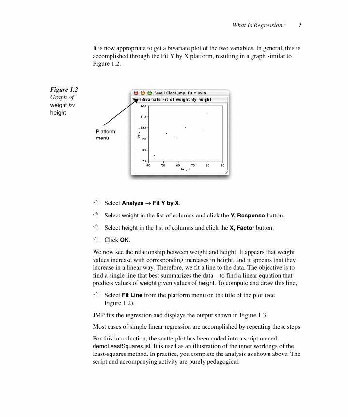
It is now appropriate to get a bivariate plot of the two variables. In general, this is accomplished through the Fit Y by X platform, resulting in a graph similar to Figure 1.2.

Select Analyze → Fit Y by X.

Select weight in the list of columns and click the Y, Response button.

Select height in the list of columns and click the X, Factor button.

Click OK.

We now see the relationship between weight and height. It appears that weight values increase with corresponding increases in height, and it appears that they increase in a linear way. Therefore, we fit a line to the data. The objective is to find a single line that best summarizes the data—to find a linear equation that predicts values of weight given values of height. To compute and draw this line,

Select Fit Line from the platform menu on the title of the plot (see Figure 1.2).

JMP fits the regression and displays the output shown in Figure 1.3.

Most cases of simple linear regression are accomplished by repeating these steps.

For this introduction, the scatterplot has been coded into a script named demoLeastSquares.jsl. It is used as an illustration of the inner workings of the least-squares method. In practice, you complete the analysis as shown above. The script and accompanying activity are purely pedagogical.

Figure 1.2 Graph of weight by height

Platformmenu


Open the script demoLeastSquares.jsl, found in the Sample Scripts folder. Note that the Open dialog must show files of type JSL, so adjust the dialog to show Data Files, JMP Files, or All Readable documents.

Select Edit → Run Script.

When the script output appears, click the Your Residuals button (shown in Figure 1.5).

This button turns on a measurement for the accuracy of the linear model. The model itself is represented by an orange line. The distance from this line to each data point is called the residual, and it is represented by the dark blue vertical lines that connect the orange line to each data point. See Figure 1.4 for an expla-nation of the graph produced by the script.

The handles are used to move the model around so that it approximates the shape of the data. As you drag one handle, the other stays fixed. Obviously, many lines can be drawn through the data, each resulting in different residual values. The question is, of all the possible lines that can be drawn through the data, which is the best?

Figure 1.3 Regression Output


One logical criterion for a “best-fitting” line could be that it is the one where the sum of the residuals is the smallest number. Or, one could claim the best-fitting line is the one that has equal numbers of points above and below the line. Or, one could choose the line that minimizes the perpendicular distances from the points to the line.

In the least-squares method, the squares of the residuals are measured. Geometri-cally, this value of (residual)2 can be represented as a square with the length of a side equal to the value of the residual.

Click the Your Squares button to activate the squares of the residuals.

It is this quantity that is minimized. The line with the smallest sum of the squared residuals is used as the best fitting. Geometrically, this means that we seek the line that has the smallest area covered by the squares superimposed on the plot. As an aid to show the sum of the squared residuals, a “thermometer” is appended to the right of the graph (Figure 1.5). This thermometer displays the total area covered by the squared residuals.

Drag the handles of the model to try to minimize the sum of the squared residuals.

Figure 1.4 demoLeast Squares Window Linear model

Draggable handles

Data points

Residuals


When you think the sum is at a minimum,

Push the LS Line and LS Squares buttons.

The actual (calculated) least-squares line is superimposed upon the graph, along with the squares of its residuals. Additionally, a line is drawn on the thermometer representing the sum of the squared residuals from this line.

Drag the handles so that the movable line corresponds exactly to the least-squares line.

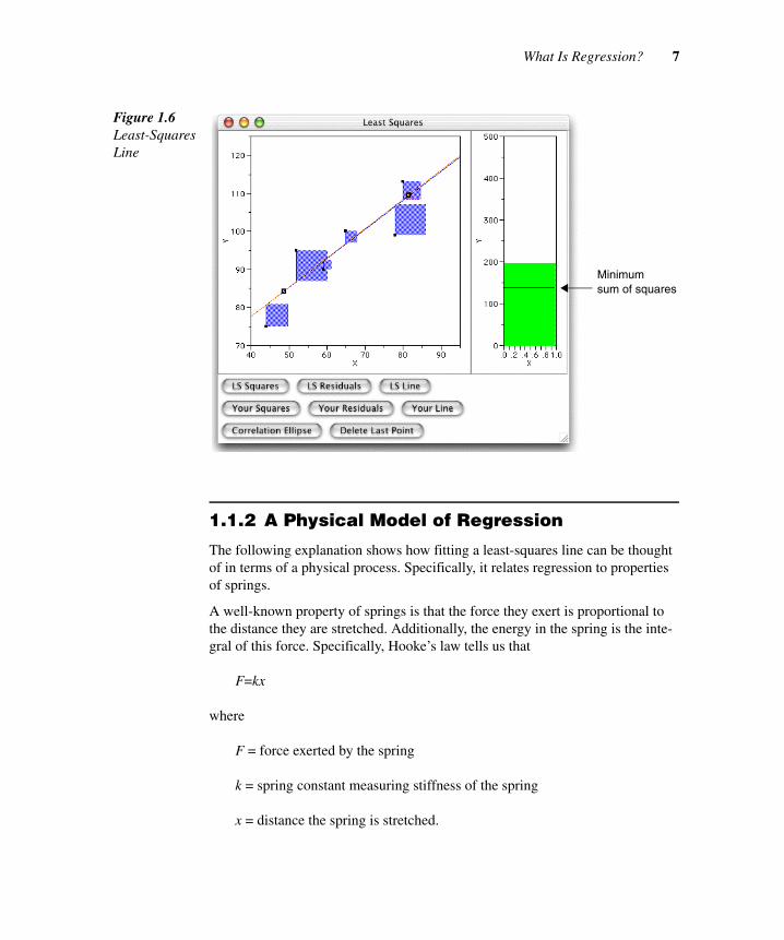
Note that the sum of squares now corresponds to the least-squares sum (Figure 1.6). You should notice that as you dragged the handles onto the least-squares line, the sum of the squared residuals decreased until it matched the min-imum sum of squares.

Drag the handles so that the movable line moves off the least-squares line. Experiment with the line moving away from the least-squares line in all directions.

This illustrates the central concept of least-squares regression. The least-squares line, often called the line of best fit, is the one that minimizes the sum of squares of the residuals.

Figure 1.5 Squared Residuals

Squaredresiduals

Sum of squared residuals


1.1.2 A Physical Model of Regression

The following explanation shows how fitting a least-squares line can be thought of in terms of a physical process. Specifically, it relates regression to properties of springs.

A well-known property of springs is that the force they exert is proportional to the distance they are stretched. Additionally, the energy in the spring is the inte-gral of this force. Specifically, Hooke’s law tells us that

F=kx

where

F = force exerted by the spring

k = spring constant measuring stiffness of the spring

x = distance the spring is stretched.

Figure 1.6 Least-Squares Line

Minimumsum of squares


For reasons that will become evident later, let the spring constant k be repre-sented by 1/σ. Then, the energy in a spring with this value of k is

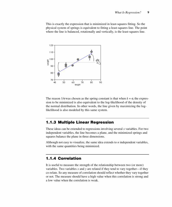
Again consider the height/weight data shown in Figure 1.1.

A graph of weight vs. height is shown here with a line drawn at the mean value of weight. Now, imagine hooking up springs, with one end on a data point and the other end on the mean line. If xi represents a data point and µ represents the value of the overall mean, then each spring is stretched a distance of xi – µ.

If the whole system were released, the mean line would rotate and shift to the point of minimum total energy in the system. Mathematically, where µ is the mean of x and σ is the standard deviation of x,

would be minimized. The constant on the outside of the sum would not come into play with a minimization, so in essence we would minimize

E1σ---x xd∫ x

2

2σ-----= =

Imagine theline heldhorizontallyunder tension

xi µ–σ

-------------

2

i 1=

n

∑ 1σ--- xi µ–( )2

i 1=

n

∑=

xi µ–( )2

i 1=

n

∑


This is exactly the expression that is minimized in least-squares fitting. So the physical system of springs is equivalent to fitting a least-squares line. The point where the line is balanced, rotationally and vertically, is the least-squares line.

The reason 1/σ was chosen as the spring constant is that when k = σ, the expres-sion to be minimized is also equivalent to the log-likelihood of the density of the normal distribution. In other words, the line given by maximizing the log-likelihood is also modeled by this same system.

1.1.3 Multiple Linear Regression

These ideas can be extended to regressions involving several x variables. For two independent variables, the line becomes a plane, and the minimized springs and squares balance the plane in three dimensions.

Although not easy to visualize, the same idea extends to n independent variables, with the same quantities being minimized.

1.1.4 Correlation

It is useful to measure the strength of the relationship between two (or more) variables. Two variables x and y are related if they tend to vary together—if they co-relate. So any measure of correlation should reflect whether they vary together or not. The measure should have a high value when this correlation is strong and a low value when the correlation is weak.


The rules of correlation mimic those of integer multiplication. Factors that are the same (either both positive or both negative) yield a positive product. Similarly, factors that are different yield a negative product. This is similar to our desired measure of correlation, so multiplication of the values of x and y is used in the correlation measure. Of course, x and y might be measured on different scales, so standardized values are used instead of actual values.

The corresponding (standardized) values for each pair are multiplied together, and a weighted average of these products is computed. Stated mathematically,

This quantity, termed the correlation coefficient and abbreviated r, measures lin-ear correlation in two variables. A similar quantity, known as the coefficient of determination and abbreviated R2, is used in measuring correlation in multiple regression. In fact, r2 = R2 for the case of simple regression.

Thinking about this formula reveals some properties of r.

❏ Switching the roles of x and y in the regression does not change the value of r, since multiplication is commutative. This does not mean that one can do something similar with the coefficients in regression. Although switching x and y values does not influence correlation, it does affect the regression equation.

❏ Changing the units of x or y does not change the correlation, since standard-ized scores are used.

❏ The correlation coefficient is sensitive to outliers, since it is based on the mean and standard deviation.

An interesting property of r is that it can be calculated through regression of the standardized variables. Figure 1.7 shows the result of a least-squares regression of standardized values of weight on standardized values of height. When the vari-ables are standardized, note that the slope of the regression line and the correla-tion coefficient are equal.

Finally, it should be noted that there are other (equivalent) formulas for comput-ing the correlation coefficient r.

r

x1 x–

sx-------------

y1 y–sy

------------ x2 x–

sx-------------

y2 y–sy

------------ …

xn x–sx

------------- yn y–

sy------------

+ + +

n 1–-----------------------------------------------------------------------------------------------------------------------------------------=


shows the relationship among the sum of the cross-products (in the numerator) and a standardization measure (in the denominator) in a similar way to the dis-cussion above.

shows the relationship between r and the slope of the regression of y on x. If the standard deviations of y and x are equivalent (as they are when both variables were standardized above), then r is equal to the slope of the regression line.

1.1.5 Seeing Correlation

The demoLeastSquares script used above can also demonstrate correlation.

If there are lines and squares still showing on the plot,

Click the buttons at the bottom of the screen to toggle all lines and squares off.

Click the LS Line button to turn on the least-squares line.

Figure 1.7 Standardized Regression

Samevalue

rx x–( ) y y–( )∑

x x–( )2y y–( )2

---------------------------------------------=

r βsxsy---=


Now, overlay a correlation ellipse and a label of the correlation coefficient.

Click the Correlation Ellipse button.

The display now appears as in Figure 1.8.

Drag one of the points in directions parallel to the least-squares line.

Notice that the line does not move much and that the correlation does not change much.

Drag one of the points in directions perpendicular to the least-squares line.

In this case, both the correlation and least-squares line change drastically. This demonstrates the effect of outliers on the correlation—and why the correlation should always be interpreted in conjunction with a graphical display of the data.

Figure 1.8 Correlation Ellipse

Drag a point inthese directions

Statistical Background 13

Similarly, points can be added to the plot close to the existing least-squares line with little effect, but single outliers can be added with great effect.

Click near and away from the regression line to add points and see their effect.

1.2 Statistical BackgroundThis section presents the rigorous definitions of many concepts involved in regression. A background in linear algebra is necessary to follow the discussion. However, it is not necessary to know all of this material to be able to use and interpret the results from JMP. Return to this section as a reference when regres-sion methods are studied in detail.

Formally, multiple linear regression fits a response variable y to a function of regressor variables and parameters. The general linear regression model has the form

y = β0 + β1x1 + ... + βmxm + ε

where

y is the response, or dependent, variable

β0, β1, ..., βm are unknown parameters

x1, x2, ..., xm are the regressor, or independent, variables

ε is a random error term.

Least squares is a technique used to estimate the parameters. The goal is to find estimates of the parameters β0, β1, ..., βm that minimize the sum of the squared differences between the actual y values and the values of y predicted by the equa-tion. These estimates are called the least-squares estimates and the quantity min-imized is called the error sum of squares.

Typically, you use regression analysis to do the following:

❏ obtain the least-squares estimates of the parameters

❏ estimate the variance of the error term

❏ estimate the standard error of the parameter estimates


❏ test hypotheses about the parameters

❏ calculate predicted values using the estimated equation

❏ evaluate the fit or lack of fit of the model.

The classical linear model assumes that the responses, y, are sampled from sev-eral populations. These populations are determined by the corresponding values of x1, x2, ..., xm. As the investigator, you select the values of the x’s; they are not random. However, the response values are random. You select the values of the x’s to meet your experimental needs, carry out the experiment with the set values of the x’s, and measure the responses. Often, though, you cannot control the actual values of the independent variables. In these cases, you should at least be able to assume that they are fixed with respect to the response variable.

In addition, you must assume the following:

1. The form of the model is correct; that is, all important independent variables are included and the functional form is appropriate.

2. The expected values of the errors (from the mean) are zero.

3. The variances of the errors (and thus the response variable) are constant across observations.

4. The errors are uncorrelated.

5. For hypothesis testing, the errors are normally distributed.

Not all regression models are necessarily linear in their parameters. For example, the model

is not linear in the parameter β2. Specifically, the term is not a linear function of β2. This particular nonlinear model, called the exponential growth or decay model, is used to represent increase (growth) or decrease (decay) over time (t) of many types of responses such as population size or radiation counts. Chapter 7, “Nonlinear Models,” is devoted to analyses appropriate for this type of model.

Additionally, the random error may not be normally distributed. If this is the case, the least squares technique is not necessarily the appropriate method for estimat-ing the parameters. One such model, the logistic regression model, is presented in the section “Binary Response Variable: Logistic Regression” on page 203.

y β1eβ2x

ε+=

eβ2x

Terminology and Notation 15

1.3 Terminology and NotationThe principle of least squares is applied to a set of n observed values of y and the

associated xj to obtain estimates , , ..., of the respective parameters β0, β1,

..., βm. These estimates are then used to construct the fitted model, or estimating equation

Many regression computations are illustrated conveniently in matrix notation. Let yi, xij, and åi denote the values of y, xj, and å, respectively, in the ith observation. The Y vector, the X matrix, and the å vector can be defined as follows:

Then the model in matrix notation is

Y = Xβ + å

where β' = (β0 β1... βm) is the parameter vector.

The vector of least-squares estimates is

and is obtained by solving the set of normal equations

X'X = X'Y

Assuming that X'X is of full rank (nonsingular), there is a unique solution to the normal equations given by

β0 β1 βm

y β0 β1x1 … βˆ

mxm+ + +=

Y

y1

.

.

.ym

X

1 x11 . . x1m

. . . . .

. . .

. . .1 xn1 . . xnm

å

ε 1

.

.

.ε m

=,=,=

â'ˆ

βˆ 0

β1

.

.

.

βˆ m

=

â


The matrix (X'X)–1 is very useful in regression analysis and is often denoted as follows:

1.3.1 Partitioning the Sums of Squares

A basic identity results from least squares, specifically,

This identity shows that the total sum of squared deviations from the mean,

is equal to the sum of squared differences between the mean and the predicted values,

plus the sum of squared deviations from the observed y’s to the regression line,

These two parts are called the regression (or model) sum of squares and the resid-ual (or error) sum of squares. Thus,

Corrected Total SS = Model SS + Residual SS

Corrected total SS always has the same value for a given set of data, regardless of the model that is used; however, partitioning into model SS and residual SS depends on the model. Generally, the addition of a new x variable to a model increases the model SS and, correspondingly, reduces the residual SS. The resid-ual, or error, sum of squares is computed as follows:

â X'X( ) 1– X'Y=

X'X( ) 1– C

c00 c01 . . . c0m

c10 c11 . . . c1m

. . . .

. . . .

cm1 cm2 . . . cmn

= =

y y–( )2∑ y y–( )2∑ y y–( )2∑+=

y y–( )2∑

y y–( )2∑

y y–( )2∑


The error, or residual, mean square

s2 = MSE = (Residual SS) / (n – m – 1)

is an unbiased estimate of σ2, the variance of the ε’s.

Sums of squares, including the various sums of squares computed by any regres-sion procedure such as the Fit Y by X and Fit Model commands, can be expressed conceptually as the difference between the regression sums of squares for two models, called complete (unrestricted) and reduced (restricted) models, respec-tively. This approach relates a given SS to the comparison of two regression mod-els.

For example, denote as SS1 the regression sum of squares for a complete model with m = 5 variables:

y = β0 + β1x1 + β2x2 + β3x3 + β4x4 + β5x5 + ε

Denote the regression sum of squares for a reduced model not containing x4 and x5 as SS2:

y = β0 + β1x1 + β2x2 + β3x3 + ε

Reduction notation can be used to represent the difference between regression sums of squares for the two models:

R(β4, β5 | β0, β1, β2, β3) = Model SS1 – Model SS2

The difference or reduction in error R(β4, β5 | β0, β1, β2, β3) indicates the increase in regression sums of squares due to the addition of β4 and β5 to the reduced model. It follows that

R(β4, β5 | β0, β1, β2, β3) = Residual SS2 – Residual SS1

which is the decrease in error sum of squares due to the addition of β4 and β5 to the reduced model. The expression

R(β4, β5 | β0, β1, β2, β3)

Residual SS Y' I X X'X( ) 1– X'–( )Y=

Y'Y Y'X X'X( ) 1– X'Y–=

Y'Y β'ˆ

X'Y–=


is also commonly referred to in the following ways:

❏ the sums of squares due to β4 and β5 (or x4 and x5) adjusted for β0, β1, β2, β3 (or the intercept and x1, x2, x3)

❏ the sums of squares due to fitting x4 and x5 after fitting the intercept and x1, x2, x3

❏ the effects of x4 and x5 above and beyond (or partialing) the effects of the intercept and x1, x2, x3.

1.3.2 Hypothesis Testing

Inferences about model parameters are highly dependent on the other parameters in the model under consideration. Therefore, in hypothesis testing, it is important to emphasize the parameters for which inferences have been adjusted. For exam-ple, R(β3 | β0, β1, β2) and R(β3 | β0, β1) may measure entirely different concepts. Similarly, a test of H0: β3 = 0 may have one result for the model

y = β0 + β1x1 + β3x3 + ε

and another for the model

y = β0 + β1x1 + β2x2 + β3x3 + ε

Differences reflect actual dependencies among variables in the model rather than inconsistencies in statistical methodology.

Statistical inferences can also be made in terms of linear functions of the parame-ters of the form

H0: Lâ0: l0β0 + l1β1 + ... + lmβm = 0

where the li are arbitrary constants chosen to correspond to a specified hypothe-sis. Such functions are estimated by the corresponding linear function

of the least-squares estimates . The variance of is

A t test or F test is used to test H0: (Lâ) = 0. The denominator is usually the residual mean square (MSE). Because the variance of the estimated function is

Lâ l0β0 l1β1 … lmβm+ + +=

β Lβ

V Lâ( ) L X'X( ) 1– L'( )σ2=


based on statistics computed for the entire model, the test of the hypothesis is made in the presence of all model parameters. Confidence intervals can be con-structed to correspond to these tests, which can be generalized to simultaneous tests of several linear functions.

Simultaneous inference about a set of linear functions L1â, ..., Lkâ is performed in a related manner. For notational convenience, let L denote the matrix whose rows are L1, ..., Lk:

Then the sum of squares

is associated with the null hypothesis

H0: L1â = ... = Lkâ = 0

A test of H0 is provided by the F statistic

F = (SS(Lâ = 0) / k) / MSE

Three common types of statistical inferences follow:

1. A test that all parameters (β1, β2, ..., βm) are zero. The test compares the fit of the complete model to that using only the mean:

F = (Model SS / m) / MSE

where

Model SS = R(β0, β1, ..., βm | β0)

The F statistic has (m, n – m – 1) degrees of freedom.

Note that R(β0, β1, ..., βm) is rarely used. For more information on no-inter-cept models, see the section “Regression through the Origin” on page 44.

2. A test that the parameters in a subset are zero. The problem is to compare the fit of the complete model

L

L1

.

.

.

Lk

=

SS Lâ= 0( ) Lâ( )' L X'X( ) 1– L'( ) Lâ( )=


y = β0 + β1x1 + ... + βgxg + βg+1xg+1 + ... + βmxm + ε

to the fit of the reduced model

y = β0 + β1x1 + ... + βgxg+ ε

An F statistic is used to perform the test

F = (R(βg+1, ..., βm | β0, β1, ..., βg) / (m – g))MSE

Note that an arbitrary reordering of variables produces a test for any desired subset of parameters. If the subset contains only one parameter, βm, the test is

F = (R(βm | β0, β1, ..., βm-1) / 1) /MSE = (partial SS due to βm) / MSE

which is equivalent to the t test

The corresponding (1 − α) confidence interval about βm is

3. Estimation of a subpopulation mean corresponding to a specific x. For a given set of x values described by a vector x, denote the population mean by µx. The estimated population mean is

The vector x is constant; hence, the variance of the estimate is

= x'(X'X)–1xσ2

This equation is useful for computing confidence intervals. A related infer-ence concerns a future single value of y corresponding to a specified x. The relevant variance estimate is

= (1 + x'(X'X)–1x)σ2

tβm

sβm

------βm

cmmMSE

-------------------------= =

βm tα 2⁄ cmmMSE±

µx β0 β1 x1 … βmxm+ + + xβ= =

µx

V µx( )

V yx

( )


1.3.3 Using the Generalized Inverse

Many applications of regression procedures involve an X'X matrix that is not of full rank and has no unique inverse. Fit Model and Fit Y by X compute a general-ized inverse (X'X)– and use it to compute a regression estimate

b = (X'X)– X'Y

A generalized inverse of a matrix A is any matrix G such that AGA = A. Note that this also identifies the inverse of a full-rank matrix.

If X'X is not of full rank, then an infinite number of generalized inverses exist. Different generalized inverses lead to different solutions to the normal equations that have different expected values; that is, E(b) = (X'X)– X'Yβ depends on the particular generalized inverse used to obtain b. Therefore, it is important to understand what is being estimated by the solution.

Fortunately, not all computations in regression analysis depend on the particular solution obtained. For example, the error sum of squares is invariant with respect to (X'X)–and is given by

SSE = Y'(1 – X(X'X)–X')Y

Hence, the model sum of squares also does not depend on the particular general-ized inverse obtained.

The generalized inverse has played a major role in the presentation of the theory of linear statistical models, notably in the work of Graybill (1976) and Searle (1971). In a theoretical setting, it is often possible, and even desirable, to avoid specifying a particular generalized inverse. To apply the generalized inverse to statistical data using computer programs, a generalized inverse must actually be calculated. Therefore, it is necessary to declare the specific generalized inverse being com-puted. For example, consider an X'X matrix of rank k that can be partitioned as

X'X =

where A11 is k × k and of rank k. Then exists, and a generalized inverse of X'X is

A11 A12

A21 A22

A111–


(X'X)– =

where each ϕij is a matrix of zeros of the same dimension as Aij.

This approach to obtaining a generalized inverse, the method used by Fit Model and Fit Y by X, can be extended indefinitely by partitioning a singular matrix into several sets of matrices as illustrated above. Note that the resulting solution to the normal equations, b = (X'X)– X'Y, has zeros in the positions corresponding to the rows filled with zeros in (X'X)–. This is the solution printed by these procedures, and it is regarded as providing a biased estimate of b.

However, because b is not unique, a linear function, Lb, and its variance are gen-erally not unique either. However, a class of linear functions called estimable functions exists, and they have the following properties:

❏ The vector L is a linear combination of rows of X.

❏ Lb and its variance are invariant through all possible generalized inverses. In other words, Lb is unique and is an unbiased estimate of Lâ.

Analogous to the full-rank case, the variance of an estimable function Lb is given by

V(Lb) = (L(X'X)– L')σ2

This expression is used for statistical inference. For example, a test of H0: Lâ = 0 is given by the t test

Simultaneous inferences on a set of estimable functions are performed in an anal-ogous manner.

A11 ϕ12

ϕ21 ϕ22

tLb

L X'X( )–L'MSE

-----------------------------------------------=

Regression with JMP 23

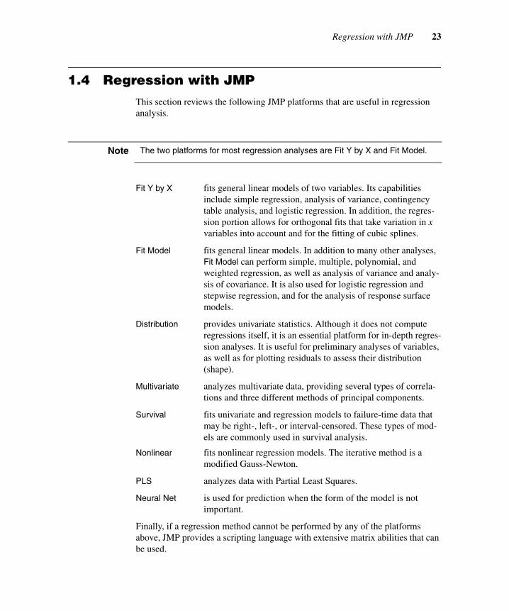
1.4 Regression with JMPThis section reviews the following JMP platforms that are useful in regression analysis.

Fit Y by X fits general linear models of two variables. Its capabilities include simple regression, analysis of variance, contingency table analysis, and logistic regression. In addition, the regres-sion portion allows for orthogonal fits that take variation in x variables into account and for the fitting of cubic splines.

Fit Model fits general linear models. In addition to many other analyses, Fit Model can perform simple, multiple, polynomial, and weighted regression, as well as analysis of variance and analy-sis of covariance. It is also used for logistic regression and stepwise regression, and for the analysis of response surface models.

Distribution provides univariate statistics. Although it does not compute regressions itself, it is an essential platform for in-depth regres-sion analyses. It is useful for preliminary analyses of variables, as well as for plotting residuals to assess their distribution (shape).

Multivariate analyzes multivariate data, providing several types of correla-tions and three different methods of principal components.

Survival fits univariate and regression models to failure-time data that may be right-, left-, or interval-censored. These types of mod-els are commonly used in survival analysis.

Nonlinear fits nonlinear regression models. The iterative method is a modified Gauss-Newton.

PLS analyzes data with Partial Least Squares.

Neural Net is used for prediction when the form of the model is not important.

Finally, if a regression method cannot be performed by any of the platforms above, JMP provides a scripting language with extensive matrix abilities that can be used.

Note The two platforms for most regression analyses are Fit Y by X and Fit Model.

1 Regression Concepts - SAS Supportsupport.sas.com/publishing/pubcat/chaps/58789.pdf · Chapter 1...

Documents

Transcript of 1 Regression Concepts - SAS Supportsupport.sas.com/publishing/pubcat/chaps/58789.pdf · Chapter 1...