1

Probability (Rosner, chapter 3)KLMED 8004, September 2010

Eirik Skogvoll, Consultant/ Professor

• What is probability?• Basic probability axioms and rules of calculation

2

Breast cancer (Example 3.1)

• Incidence of breast cancer during the next 5 years for women aged 45 to 54– Group A had their first birth before the age of 20 (“early”)– Group B had their first birth after the age of 30 (“late”)

• Suppose 4 out of 1000 in group A, and 5 out of 1000 i group B develop breast cancer over the next 5 years. Is this a chance finding, or does it represent a genuine increased risk?

• If the numbers were 40 out of 10 000 and 50 out of 10 000? Still due to chance?

3

Diagnostic test (Eks 3.26)

• Suppose that an automated blood pressure machine classifies 85% of hypertensive patients as hypertensive,23% of normotensive patients as hypertensive, and we know that 20% of the general population are hypertensive.

• What is the sensitivity, specificity and positive predictive value of the test?

4

Probability of male livebirth – expl. 3.2

Number of livebirths

Number of boys

Proportion of boys

10 8 0,8 100 55 0,55 1000 525 0,525 10000 5139 0,5139 100000 51127 0,51127 3760358 1927054 0,51247 17989361 9219202 0,51248 34832051 17857857 0,51268

5

Probability (Def 3.1)

• The sample space, S (N: “utfallsrommet”) is the set of all possible outcomes from an experiment

• An experiment is repeated n times.The event A occurs nA times.The relative frequency nA/n approaches a fixed number as the number of experiments (trials) goes towards infinity. This number Pr(A) is called the Probability of A.

• This definition is termed frequentist.

6

How to quantify probability

• Empirical estimation: nA/n

• Inference/ calculations based on a theoretical/ physical model• ”Subjective” probability

”Probability has no universally accepted interpretation”

Chatterjee, S. K. Statistical Thought. A perspective and History. Oxford University Press, 2003. Page 36.

7

Example: throw a die

• Probability of a six is 1/6• Probability of five or six is 2/6• These calculations are made under assumptions of fair dice (equal

probabiltiy of all outcomes) and certain rules of calculation.

8

”There is hardly any way back, says the UN climate committee. There is a a 50 percent chance that polar meltdown is inevitable, an April report claims.

”The UN climate comittee presented their latest report in January. The committe states that there is a 90 percent chance that global warming is caused by human activity”

http://www.aftenposten.no/nyheter/miljo/article1650116.ece(19.02.2007)

(Very) subjective probability:

9

http://weather.yahoo.com/accessed 31. August 2010 at 1111 hours

Tonight: A steady rain early...then remaining cloudy with a few showers. Low 43F. Winds WNW at 5 to 10 mph. Chance of rain 80%. Rainfall near a quarter of an inch.

10

Mutually exclusive events (Def 3.2)

• Two events A og B are mutually exclusive (N: “disjunkte”) if they cannot both happen at the same time

11

Expl. 3.7 Diastolic blood pressure (DBP)

• A = {DBP 90}• B = {75 DBP 100}

• A og B are not mutually exclusive

12

A B (“A union B”) means that A, or B,or both, occur (Def 3.4).

13

Example

• A = {DBP 90}• B = {75 DBP 100}

• A B = {DBP 75}

14

A B (“Intersection”, N: “Snitt”) means that both A and B occurs(Def. 3.5)

15

Example

• A = {DBP 90}• B = {75 DBP 100}

• A B = {90 DBP 100}

16

Basic rules of probabilityKolmogorov’s axioms (1933, Eq. 3.1)

• The probability of an event, E, always satisfies:

0 Pr(E) 1

• If A and B are mutually exclusive, then Pr(A B) = Pr(A) + Pr(B)This also applies to more than 2 events.

• The probability of a certain event is 1: Pr(S) = 1

17

Example (Rosner, expl 3.6, s.47), diastolic BP

A: DBP < 90 mmHg (normal). Pr (A) = 0,7

B: 90 DBT < 95 (“borderline”). Pr (B) = 0,1

C: DBT < 95

Pr (C) = Pr(A B) = Pr (A) + Pr (B) = 0,7 + 0,1 = 0,8

Because mutually exclusive

18

A ("complement of A") means that A does not occur.

(Def 3.6)

Pr(A) = 1 - Pr(A)

19

Independent events

• “A og B are independent if Pr(B) is not influenced by whether A has happened or not.”

• Def 3.7: A and B are independent if

Pr(A B) = Pr(A) Pr(B)

20

Example 3.15

Testing for syphilis

= {Dr A makes a positive diagnosis}

= {Dr B makes a positive diagnosis}

Given that

Pr( ) 0,1 Pr( ) 0,17 Pr( ) 0,08

Then

Pr( ) 0,08 > Pr( ) Pr(

A

B

A B A B

A B A B

) 0,1 0,17 0,017

and the events are dependent (as expected)

21

The multiplication law of probability(Equation 3.2)

• If A1, …, Ak are independent, then

Pr(A1 A2 ... Ak) = Pr(A1)Pr(A2)…Pr(Ak)

22

The addition law of probability (Eq. 3.3)

• Pr(AB) = Pr(A) + Pr(B) - Pr(AB)

Don’t count this set twice!

Rosner fig. 3.5, s. 52

23

Example 3.13 and 3.17

A= {Mother’s DBP 95} B = {Father’s DBP 95}

Pr (A) = 0,1 Pr (B) = 0,2 Assume independence.

What is the probability of being a “hypertensive family”?

Pr(AB) = Pr(A)*Pr(B) = 0,1*0,2 = 0,02

What is the probability of at least one parent being hypertensive?

Pr (A B) = Pr (A) + Pr (B) - Pr(AB)

= 0,1 + 0,2 - 0,02 = 0,28

24

Consider three independent events A, B and C

Pr (A B C) = Pr (A) + Pr (B) + Pr (C)

- Pr (A B) - Pr (A C) - Pr (B C) + Pr (A B C)

AB

C

S

Addition theorem for 3 events

25

Population 4 000 000

4 500

New cancer within 1 year

A15 000

B300 000

Age 70-79 year

4500( | ) 1.5%

300000P A B

4500 / 4000000 ( )( | )

300000 / 4000000 ( )

P A BP A B

P B

Conditional probability – Aalen et al. (2006)

A = ”This person develops cancer within 1 year” 15 000 0.38%

4 000 000P(A) =

B = ”The person is 70-79 years old”30 0000

4 000 000P(B)

26

Conditional probability - def 3.9

• Conditional probability of B given A:

• We “re-define” the sample space from S to A:

• Pr(B|A) = Pr(A B)/Pr(A)

27

Conditional probability and independence

A and B are independent if and only if (Eq. 3.5 )

(1) Pr(B|A) = Pr(B)

Then also Pr(B|A) Pr(B), and the corresponding for A|B.

(1) may be used as a definition of independence!

28

Example 3.20 (cont. expl 3.15)

Pr( | ) Pr( ) / Pr( ) 0,08 / 0,01 0,8

Pr( )=0,17 - events are dependent

Pr( | ) Pr( ) / Pr( )

Pr( ) Pr( ) Pr( ) because mutually exclusiv

B A B A A

B

B A B A A

B B A B A

e

så

Pr( | ) (Pr( ) Pr( )) / Pr( ) (0,17 0,08) / 0,9 0,1

B A B B A A

29

Another look at problem 3.1 +++

Father ill (A2)

Father healthy

Total

Mother ill (A1)

2 8 10

Mother healthy

8 82 90

Totalt 10 90 100

A 2 by 2 table of 100 families:

Note the difference of (A1 A2) og (A1|A2 ) …(A1 A2) are defined on S (the entire sample space) while (A1|A2) is defined on A2 as the sample space

30

Relative risk

Relative risk (RR) of B given A (def 3.10):

Pr(B|A)RR =

Pr(B|A)

If A are B independent, RR=1 (by definition)

31

Relative risk - eks 3.19

A = {Positive mammography}

B = {Breast cancer the next 2 years}

Pr(B|A) = 0,1

Pr(B|A) = 0,0002

Pr(B|A) 0,1RR = = = 500

0,0002Pr(B|A)

32

Dependent events (expl 3.14 →)

• A = {Mother’s DBP 95},

• B = {First born child’s DBP 95}

• Pr(A) = 0,1 Pr(B) = 0,2 Pr(AB) = 0,05 (known!)

• Pr(A)*Pr(B) = 0,1*0,2 = 0,02

Pr(AB) thus: the events are dependent!

• Pr(B|A) = Pr(AB)/Pr(A) = 0,05/0,1 = 0,5 Pr(B)

33

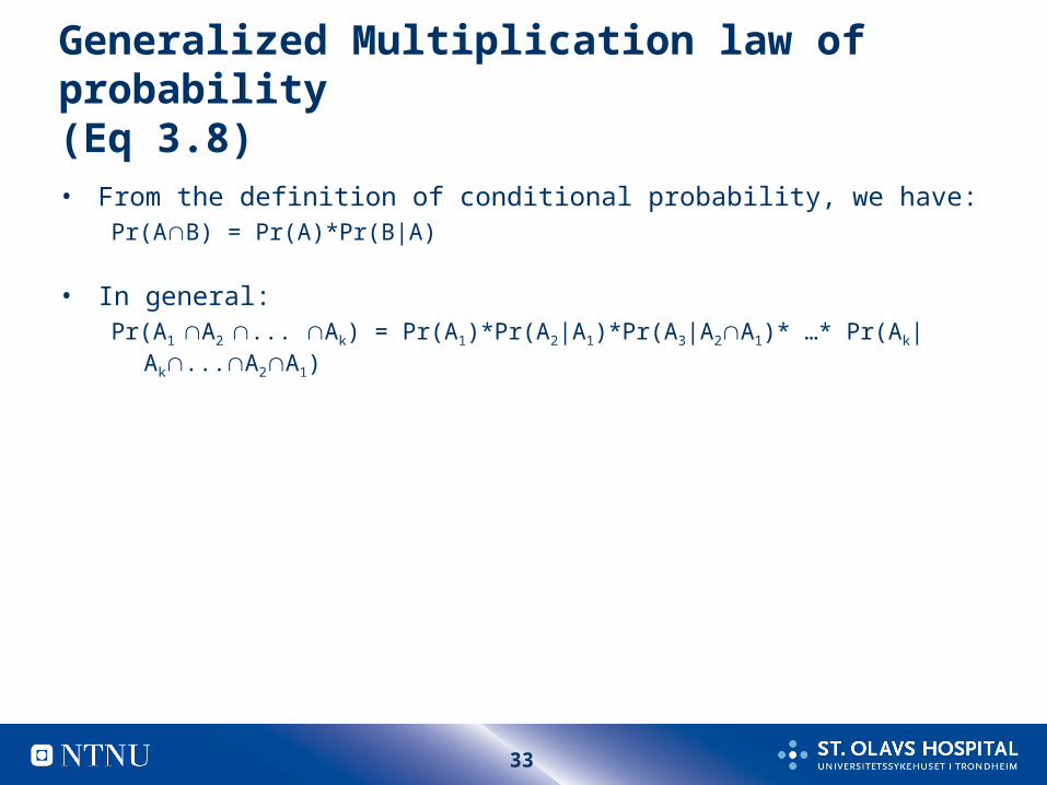
Generalized Multiplication law of probability(Eq 3.8)

• From the definition of conditional probability, we have:Pr(AB) = Pr(A)*Pr(B|A)

• In general:Pr(A1 A2 ... Ak) = Pr(A1)*Pr(A2|A1)*Pr(A3|A2A1)* …* Pr(Ak|Ak...A2A1)

34

A1A2

Ak

B

1

Pr( ) Pr( | ) Pr( )k

i ii

B B A A

Total-Probability Rule (Eq 3.7)

35

Prevalence

• The prevalence of a disease equals the proportion of population that is diseased (def 3.17)

• Expl. (Aalen, 1998): – By 31. December 1995, 21 482 Norwegian women suffered from breast

cancer.

– Total female population: 2 150 000

– Prevalence: 21 482 / 2 150 000 = 0,010 ( 1 %)

36

Incidence (or incidence rate)

• Incidence is a measure of the number of new cases occurring during some time period (i.e. a rate)

• Expl (Aalen, 1998): – During 1995, a total of 2 154 Norwegian women were diagnosed with

breast cancer

– Total female population: 2 150 000

– Incidence rate: 2 154 cases/ (2 150 000 persons * 1 year) = 0,0010 cases per person and year

37

0.024*0.450+ 046*0.280 +0.088* 0.20+ 0,153*0,070 = 0.052

Prevalence of cataract - expl 3.22

We wish to determine the total prevalence of cataract in the population ≥ 60 years during the next 5 years. Age specific prevalence is known. A1 = {60-64 yrs}, A2 = {65-69 yrs}, A3 = {70-74 yrs}, A4 = {75+ yrs}, B = {catarakt within 5 år}

Pr(A1)=0,45, Pr(A2)=0,28, Pr(A3)=0,20, Pr(A4)=0,07 Pr(B|A1)=0,024, Pr(B|A2)=0,046, Pr(B|A3)=0,088, Pr(B|A4)=0,153

i=1

Pr(B) = Pr (B|Ai)*Pr(Ai)k

38

Eks: Age adjusted incidenc of breast cancer, www.kreftregisteret.no

Age-adjusted incidence rate 1954– 99 (world std.)Breast, females

0

20

40

60

80

1954 1959 1964 1969 1974 1979 1984 1989 1994 1999

Year of diagnosis

Rate per100 000

39

Bayes’ rule, diagnosis and screening

A {symptom or positive diagnostic test}

B {disease}

P(B) disease prevalence

P(A|B) sensitivity

P(A|B) " false positive rate"

P(A|B) spesificity

P(A|B) P(A|B) 1 (why?)

P(A|B) 1 P(A|B) 1 specificity

P

(B|A) PPV PV positive predictive value

P(B|A) NPV PV negative predictive value

B

BA

S

40

Diagnosis of breast cancer (expl 3.23)

A = {pos. mammogram}

B = {breast cancer within 2 years}

PV PPV 0,1A)|(BPr

0,9998 PV NPV Dvs.

0,9998 0,00021 )A|B(Pr 0002,0)A|(BPr

41

Bayes’ rule

)BP( )B|P(A(B)Pr B)|(APr

(B)Pr B)|(APr

(A)Pr

A)(BPr A)|P(BPV PPV

Definition (Rosner Eq. 3.9) Bayes’ rule/ theoremCombines the expressions of conditional and total probability:

We have found one conditional probability by means of the “opposite” or “inverse” conditional probability!

B

BA

S

42

Bayes’ rule

Example (Rosner expl. 3.26, s. 61)

Prevalence of hypertension = Pr (B) = 0,2. The auto-BP machine classifies 84 % of hypertensive patients and 23 % of normotensive patients as hypertensive. PPV? NPV?

Pr (A|B) 0,84 (sensitivity)

og Pr ( | ) 0,23 ("false positive rate")

dvs. spesificity Pr (A | B) 1 0,23 0,77

A B

43

-

From Bayes' rule we have

Pr( | ) Pr( )PV Pr( | )

Pr( | ) Pr( ) Pr( | ) Pr( )

(1 ) (1 )

0,84 0,2 0,1680,48

0,84 0,2 0,23 0,8 0,352

and similarly

PV Pr( | )

A B BB A

A B B A B B

sens prevalence

sens prevalence spes prevalence

sB A

(1 )

(1 ) (1 )

0,77 0,8 0,6160,95

0,77 0,8 0,16 0,2 0,648

pec prevalence

spec prevalence sens prevalence

44

Bayes’ rule. Low prevalence – a paradox?

What if the prevalence is low?

Pr(B) = 0,0001

P(A|B) = 0,84 (sensitivity)

P(A|B) 0,77 (specificity)

Then

0,84 0,0001PPV = = 0,0037

0,84 0,0001 + (1-0,77)(1-0,0001)

0,77 (1 0,0001)NPV =

0,77 (1 0,0001) + (

= 0,9999981-0,84) 0,0001

45

Bayes’ rule, diagnosis and screening

Traditional 2*2 table Illness + – Test + a [TP] b [FP] a + b result – c [FN] d [TN] c + d a + c b + d a + b + c + d

A = {test positive}, B = {illness}, TP = true positive, FP = false positive, FN = false negative, TN = true negative

46

dcba

daAccuracy

dc

dABPNPV

ba

aABPPPV

db

dBAPySpesificit

ca

aBAPySensitivit

dcba

caP(B)valence

)|(

)|(

)|(

)|(

Pre

Using a 2*2 table require us to “invent” patients on order to calculate PPV etc. …!

With Bayes’ rule this information is utilised directly.

47

Diagnostics/ ROC

Rosner tbl. 3.2 og 3.3, s. 63-64

Criterium “1+”: all rated 1 to 5 are diagnosed as abnormal. We find all the diseased, but identify none as healthy. Sensitivity = 1, spesificity = 0, ‘false positive rate’ = 1.

48

Diagnostics/ ROC

Criterium “2+”: all rated 2 til 5 are diagnosed as abnormal.We find 48/51 diseased, and identify 33/58 as healthy. Sensitivity = 0,94 Specificity = 0,57 ‘False positive rate’ = 0,43

49

Diagnostics/ ROC

Criterium “3+”: all rated 3 to 5 are diagnosed as abnormal. We find 46/51 diseased, and identify 39/58 as healthy.Sensitivity = 0,90 Spesificity = 0,67 ‘False positive rate’ = 0,33

50

Diagnostics/ ROC

Criterium “4+”: all rated 4 and 5 are diagnosed as abnormal. We find 44/51 diseased, and identify 45/58 as healthy.Sensitivity = 0,86 Specificity = 0,78 ‘False positive rate’ = 0,22

51

Diagnostics/ ROC

Criterium “5+”: all rated 5 are diagnosed as abnormal. We find 33/51 diseased, and identify 56/58 as healthy.Sensitivity = 0,65 Specificity = 0,97 ‘False positive rate’ = 0,03

52

Diagnostics/ ROC

Criterium “6+”: All rated > 5 are diagnosed as abnormal (nonsense!). We find no diseased and identify everybody as healthy. Sensitivity = 0 Specificity = 1 ‘False positive rate’ = 0

53

Diagnostics/ ROC (receiver operating characteristic)

‘False pos. rate’ 1

0,430,330,220,03

0

The result is summarized as a table ...: (Rosner table 3.3, s. 64)

… and shown as a ROC curve. (Rosner fig. 3.7, s. 64) “Cut-off” values may be decided from visual inspection.

54

Area under the ROC curve

• Summarizes overall diagnostic performance• Corresponds to the probability that a diseased patient is correctly

classified, compared to a healthy patient• Equals 1 for a perfect test• Equals 0,5 for a non-informative test• Equals 0,89 in the example