1 Probability Models for Distributions of Discrete Variables.
85
1 Probability Models for Distributions of Discrete Variables
-
date post
22-Dec-2015 -
Category
Documents
-
view
223 -
download
0
Transcript of 1 Probability Models for Distributions of Discrete Variables.
1
Probability Models for Distributions of Discrete Variables
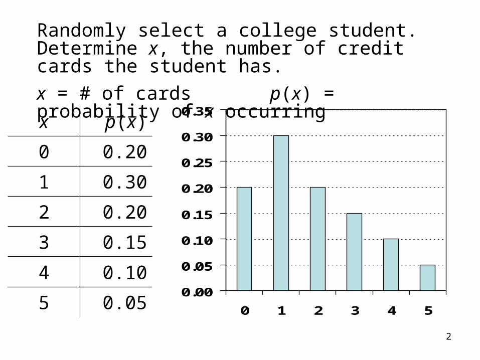
2
x p(x)
0 0.20
1 0.30
2 0.20
3 0.15
4 0.10
5 0.05
Randomly select a college student. Determine x, the number of credit cards the student has.
x = # of cards p(x) = probability of x occurring
0.00
0.05
0.10
0.15
0.20
0.25
0.30
0.35
0 1 2 3 4 5
3
A population is a collection of all units of interest.Example: All college students
A sample is a collection of units drawn from the population.
Example: Any subcollection of college students.
Probabilities go with populations.
Scientific studies randomly sample from the entire population.
Each unit in the sample is chosen randomly.
The entire sample is random as well.
Populations / Samples
4
For discrete data, a population and a sample are summarized the same way (for instance, as a table of values and accompanying relative frequencies).
A probability distribution (or model) for a discrete variable is a description of values, with each value accompanied by a probability.
Probability Models and Populations
5
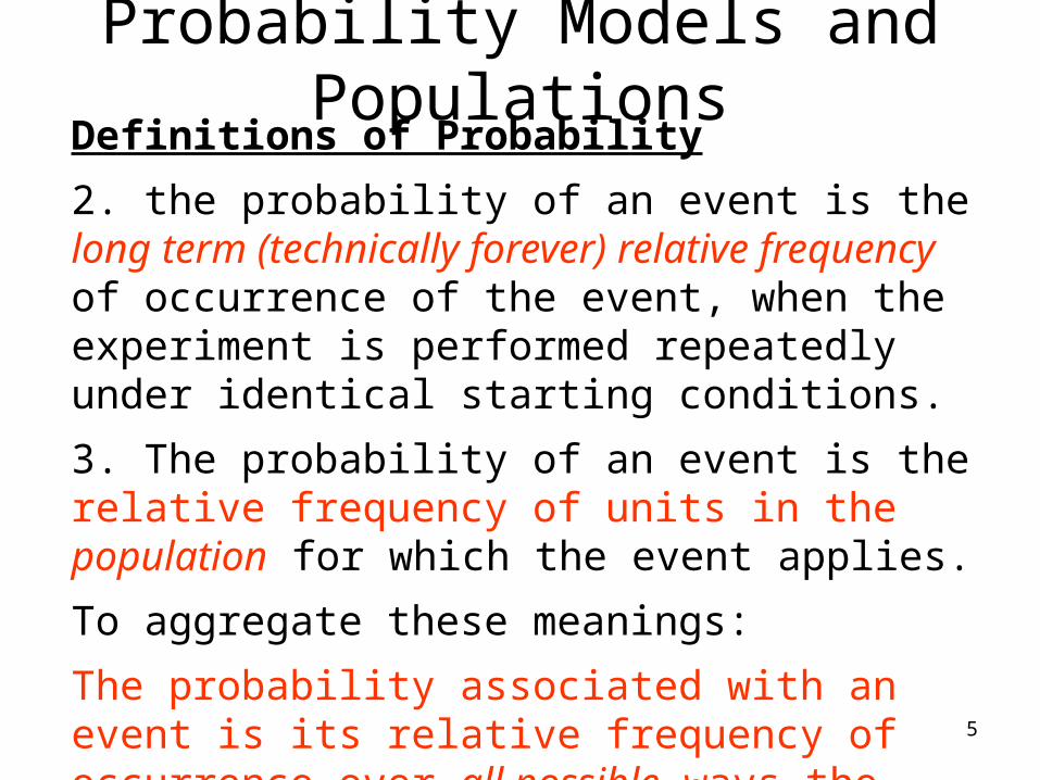
Definitions of Probability
2. the probability of an event is the long term (technically forever) relative frequency of occurrence of the event, when the experiment is performed repeatedly under identical starting conditions.
3. The probability of an event is the relative frequency of units in the population for which the event applies.
To aggregate these meanings:
The probability associated with an event is its relative frequency of occurrence over all possible ways the phenomena can take place.
Probability Models and Populations
6
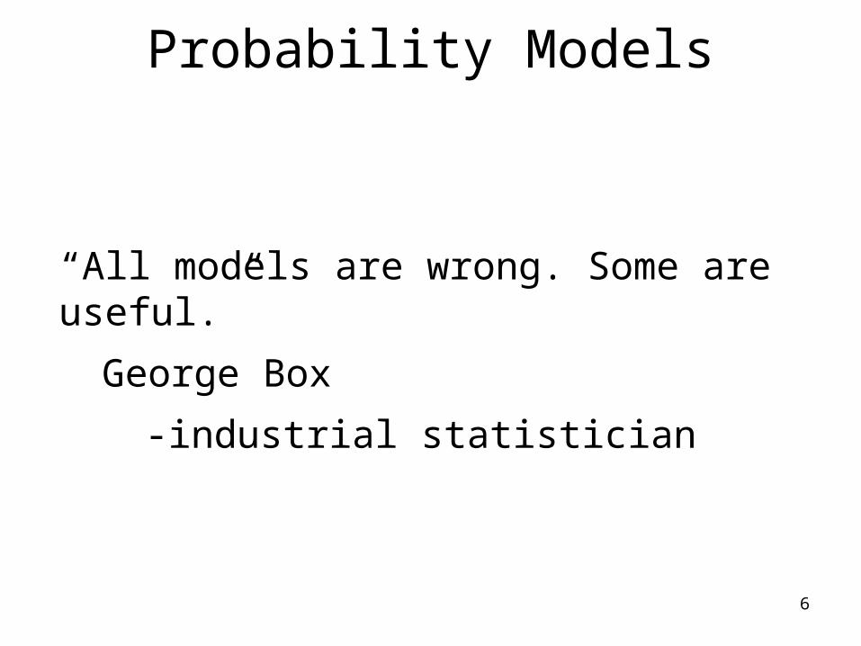
“All models are wrong. Some are useful.”
George Box
-industrial statistician
Probability Models
7
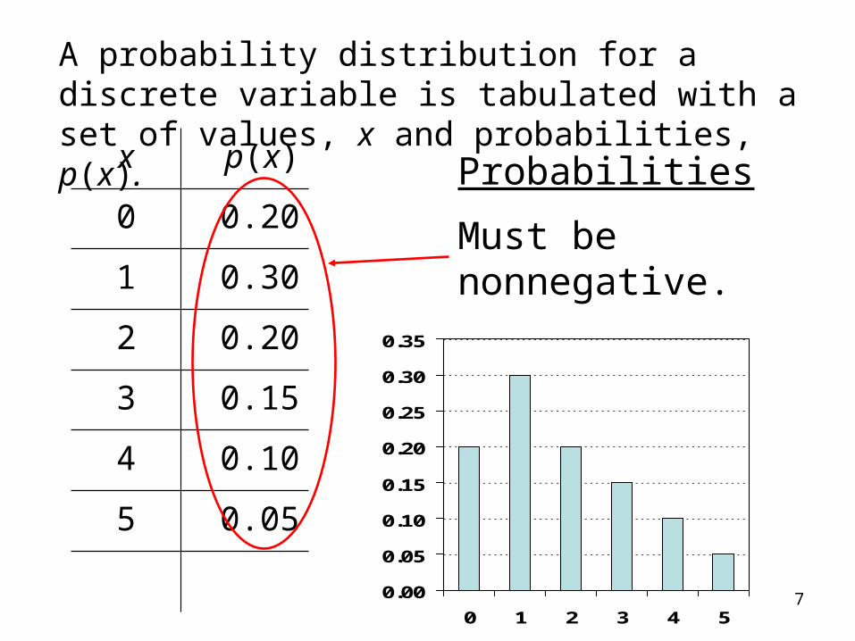
A probability distribution for a discrete variable is tabulated with a set of values, x and probabilities, p(x).
x p(x)
0 0.20
1 0.30
2 0.20
3 0.15
4 0.10
5 0.05
Probabilities
Must be nonnegative.
0.00
0.05
0.10
0.15
0.20
0.25
0.30
0.35
0 1 2 3 4 5
8
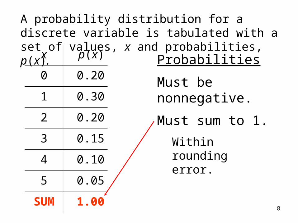
A probability distribution for a discrete variable is tabulated with a set of values, x and probabilities, p(x).
x p(x)
0 0.20
1 0.30
2 0.20
3 0.15
4 0.10
5 0.05
SUM 1.00
Probabilities
Must be nonnegative.
Must sum to 1.
Within rounding error.
9
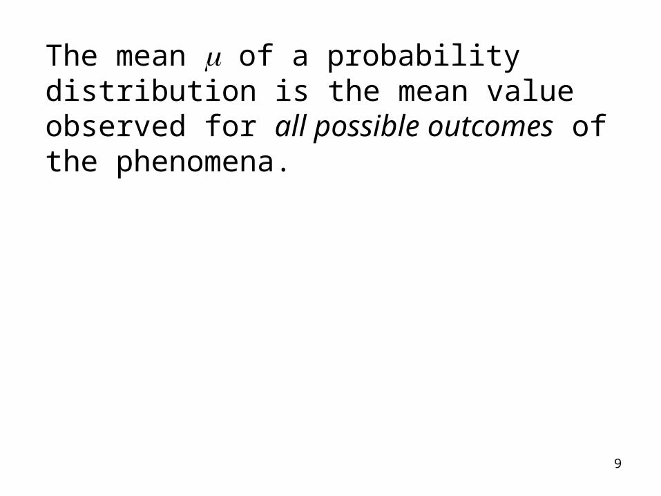
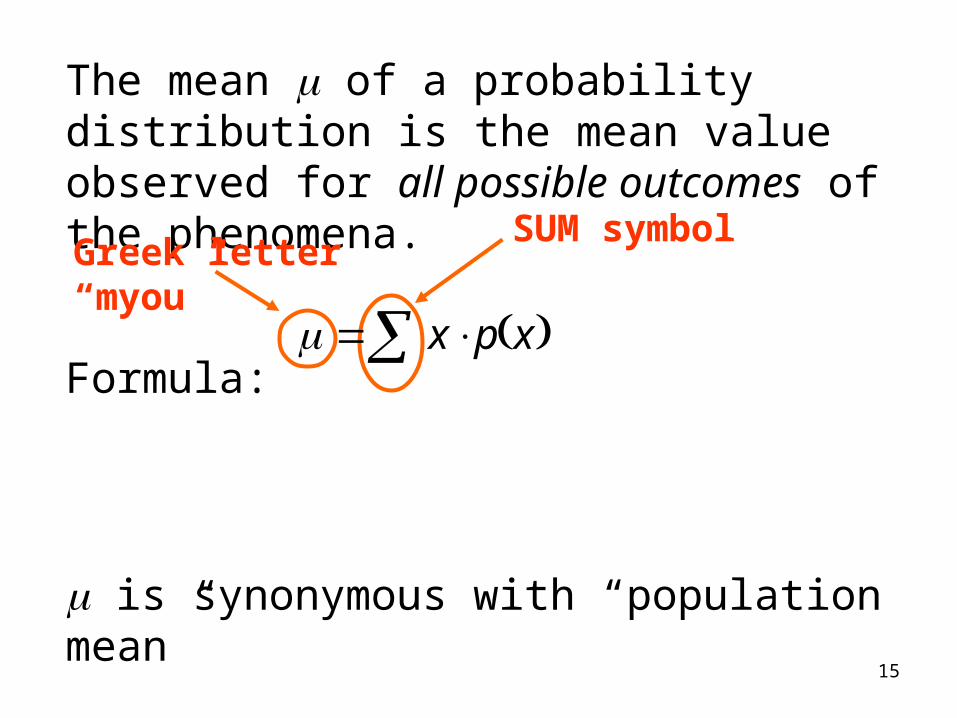
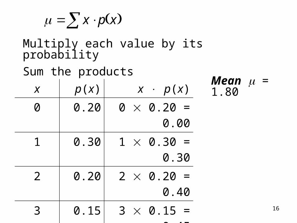
The mean of a probability distribution is the mean value observed for all possible outcomes of the phenomena.
10
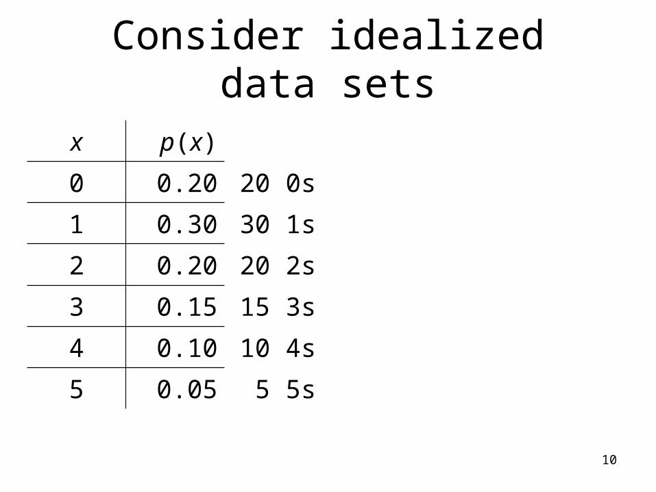
Consider idealized data sets
x p(x)
0 0.20 20 0s
1 0.30 30 1s
2 0.20 20 2s
3 0.15 15 3s
4 0.10 10 4s
5 0.05 5 5s
11
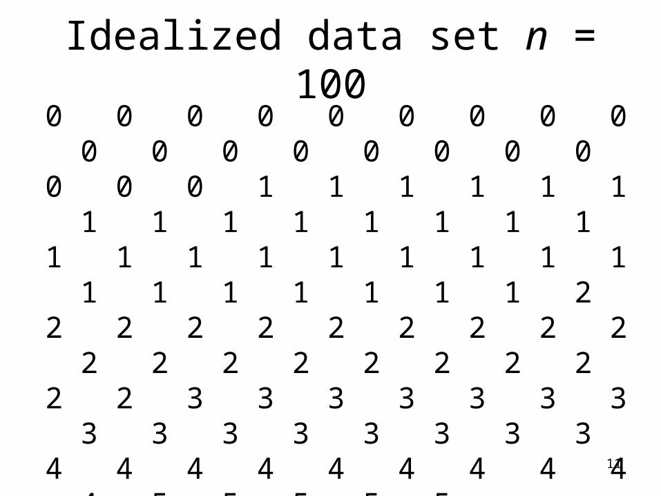
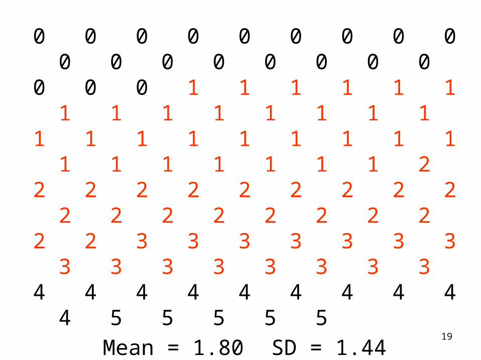
Idealized data set n = 1000 0 0 0 0 0 0 0 0 0 0 0 0 0 0 0 0 0 0 0 1 1 1 1 1 1 1 1 1 1 1 1 1 1 1 1 1 1 1 1 1 1 1 1 1 1 1 1 1 1 2 2 2 2 2 2 2 2 2 2 2 2 2 2 2 2 2 2 2 2 3 3 3 3 3 3 3 3 3 3 3 3 3 3 3 4 4 4 4 4 4 4 4 4 4 5 5 5 5 5
Mean = 1.80 SD = 1.44
12
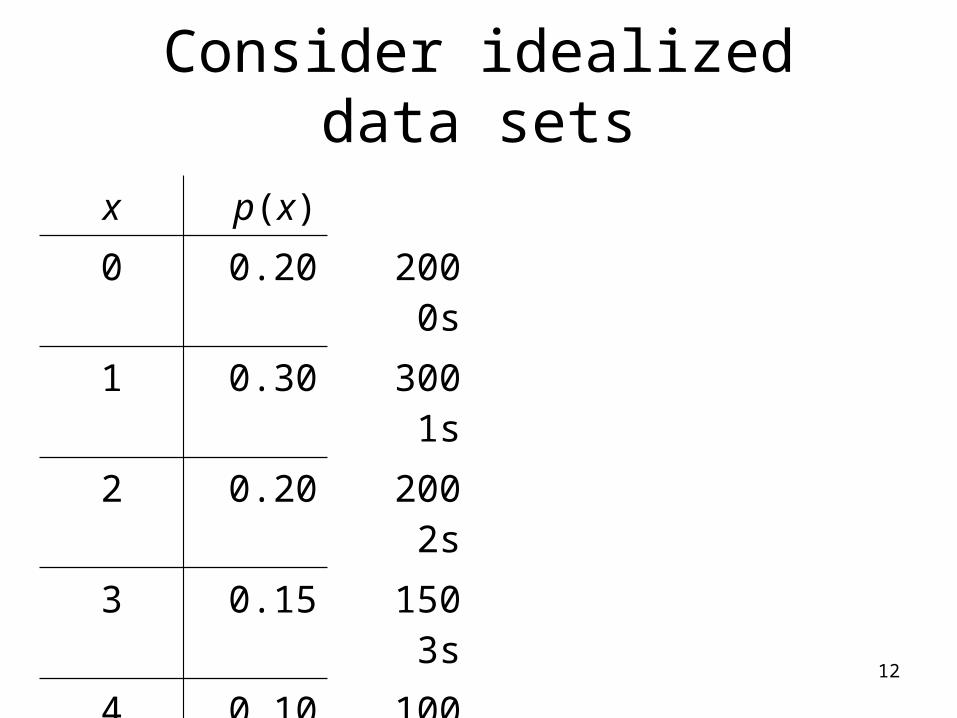
Consider idealized data sets
x p(x)
0 0.20 200 0s
1 0.30 300 1s
2 0.20 200 2s
3 0.15 150 3s
4 0.10 100 4s
5 0.05 50 5s
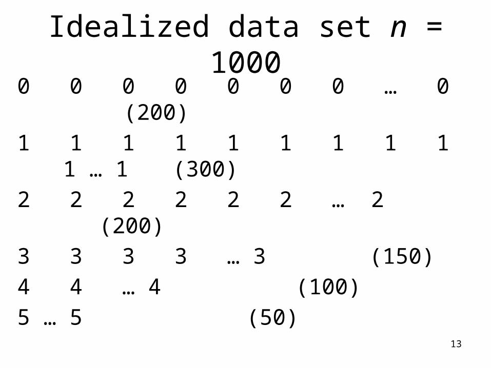
13
Idealized data set n = 10000 0 0 0 0 0 0 … 0
(200)
1 1 1 1 1 1 1 1 1 1 … 1 (300)
2 2 2 2 2 2 … 2 (200)
3 3 3 3 … 3 (150)
4 4 … 4 (100)
5 … 5 (50)
Mean = 1.80 SD = 1.44

14
Values for the mean and standard deviation don’t depend on the number of data values; they depend instead on the relative location of the data values – they depend on the distribution in relative frequency terms.
15
The mean of a probability distribution is the mean value observed for all possible outcomes of the phenomena.
Formula:
is synonymous with “population mean”
xpx
SUM symbolGreek letter “myou”
16
x p(x) x p(x)
0 0.20 0 0.20 = 0.00
1 0.30 1 0.30 = 0.30
2 0.20 2 0.20 = 0.40
3 0.15 3 0.15 = 0.45
4 0.10 4 0.10 = 0.40
5 0.05 5 0.05 = 0.25
1.00 1.80
xpx
Multiply each value by its probability
Sum the products
Mean = 1.80
17
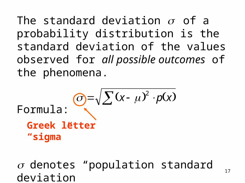
The standard deviation of a probability distribution is the standard deviation of the values observed for all possible outcomes of the phenomena.
Formula:
denotes “population standard deviation”
xpx 2
Greek letter “sigma”
18
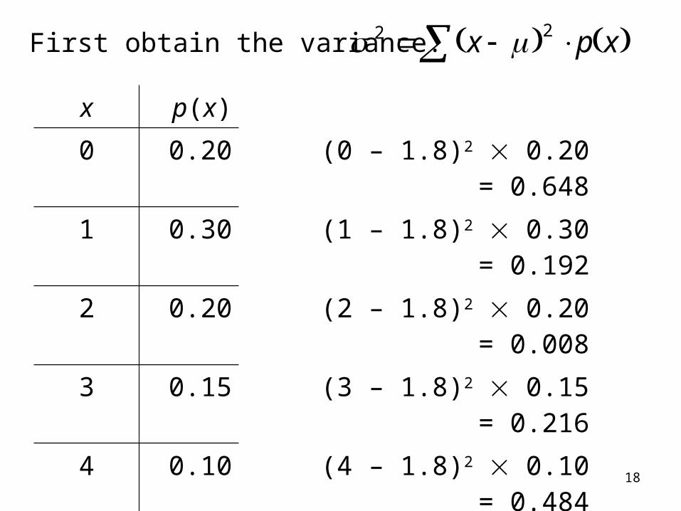
First obtain the variance. xpx 22
x p(x)
0 0.20 (0 – 1.8)2 0.20 = 0.648
1 0.30 (1 – 1.8)2 0.30 = 0.192
2 0.20 (2 – 1.8)2 0.20 = 0.008
3 0.15 (3 – 1.8)2 0.15 = 0.216
4 0.10 (4 – 1.8)2 0.10 = 0.484
5 0.05 (5 – 1.8)2 0.05 = 0.512
2 = 2.060
(take square root to obtain)
= 1.44
19
0 0 0 0 0 0 0 0 0 0 0 0 0 0 0 0 0 0 0 0 1 1 1 1 1 1 1 1 1 1 1 1 1 1 1 1 1 1 1 1 1 1 1 1 1 1 1 1 1 1 2 2 2 2 2 2 2 2 2 2 2 2 2 2 2 2 2 2 2 2 3 3 3 3 3 3 3 3 3 3 3 3 3 3 3 4 4 4 4 4 4 4 4 4 4 5 5 5 5 5
Mean = 1.80 SD = 1.44
Mean – SD = 0.56 Mean + SD = 3.24
65 / 100 = 65%
20
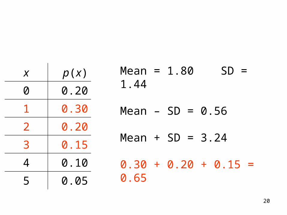
x p(x)
0 0.20
1 0.30
2 0.20
3 0.15
4 0.10
5 0.05
Mean = 1.80 SD = 1.44
Mean – SD = 0.56
Mean + SD = 3.24
0.30 + 0.20 + 0.15 = 0.65

21
x = # children in randomly selected college student’s family.
0.00
0.05
0.10
0.15
0.20
0.25
0.30
1 2 3 4 5 6 7 8 9 10
# of Children
Pro
bab
ilit
y
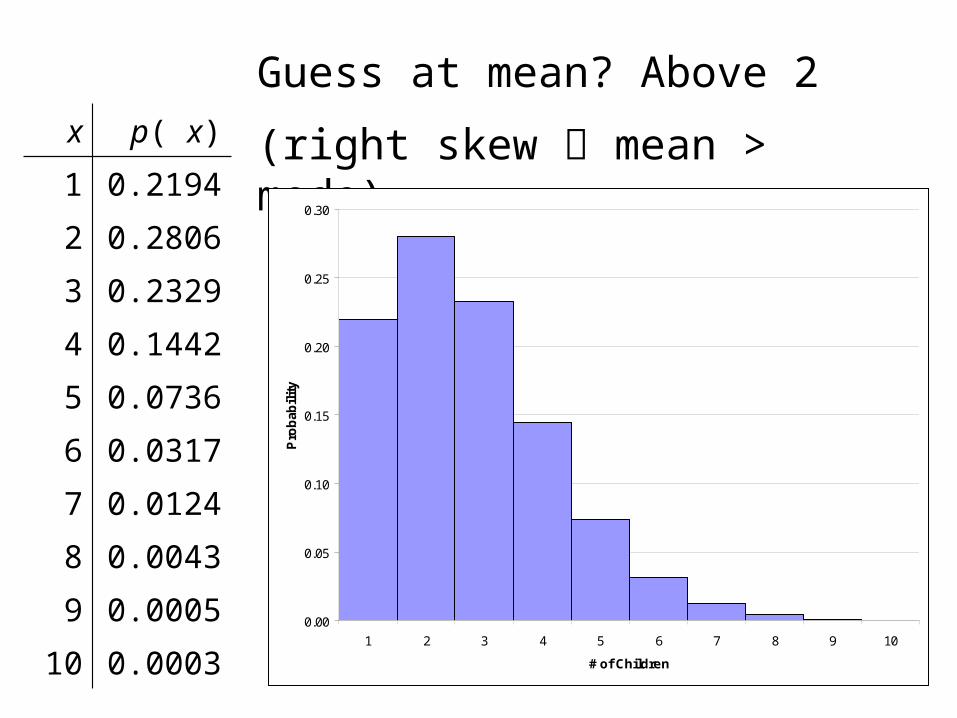
x p( x)
1 0.2194
2 0.2806
3 0.2329
4 0.1442
5 0.0736
6 0.0317
7 0.0124
8 0.0043
9 0.0005
10 0.0003

22
x = # children in randomly selected college student’s family.
0.2194 = 21.94% of all college students come from a 1 child family.
x p( x)
1 0.2194
2 0.2806
3 0.2329
4 0.1442
5 0.0736
6 0.0317
7 0.0124
8 0.0043
9 0.0005
10 0.0003
23
Guess at mean? Above 2
(right skew mean > mode).
0.00
0.05
0.10
0.15
0.20
0.25
0.30
1 2 3 4 5 6 7 8 9 10
# of Children
Pro
bab
ilit
y
x p( x)
1 0.2194
2 0.2806
3 0.2329
4 0.1442
5 0.0736
6 0.0317
7 0.0124
8 0.0043
9 0.0005
10 0.0003
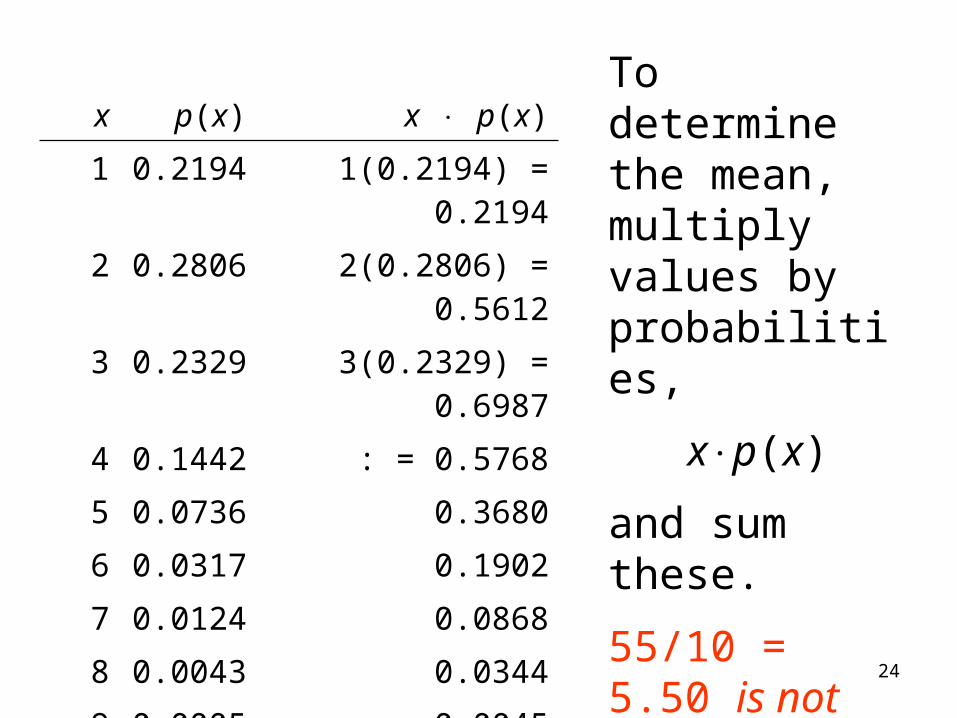
24
To determine the mean, multiply values by probabilities,
xp(x)
and sum these.
55/10 = 5.50 is not the mean
1.000/10 = 0.10 is not the mean
x p(x) x p(x)
1 0.2194 1(0.2194) = 0.2194
2 0.2806 2(0.2806) = 0.5612
3 0.2329 3(0.2329) = 0.6987
4 0.1442 : = 0.5768
5 0.0736 0.3680
6 0.0317 0.1902
7 0.0124 0.0868
8 0.0043 0.0344
9 0.0005 0.0045
10 0.0003 0.0030
55 1.0000 Mean: = 2.7430
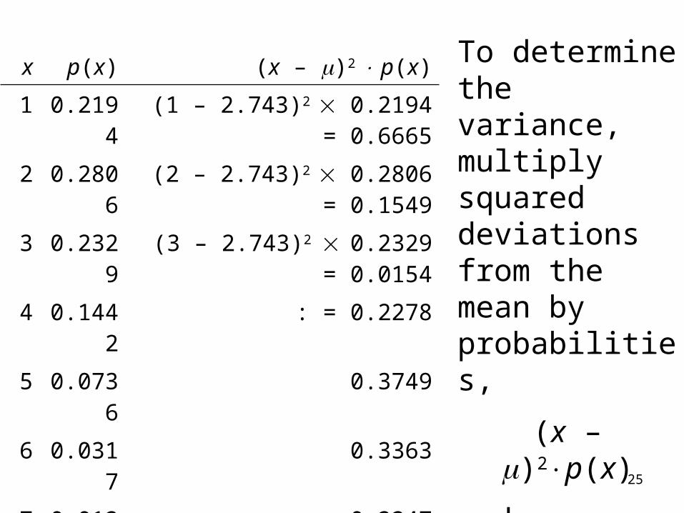
25
To determine the variance, multiply squared deviations from the mean by probabilities,
(x – )2p(x)
and sum these.
x p(x) (x – )2 p(x)
1 0.2194 (1 – 2.743)2 0.2194 = 0.6665
2 0.2806 (2 – 2.743)2 0.2806 = 0.1549
3 0.2329 (3 – 2.743)2 0.2329 = 0.0154
4 0.1442 : = 0.2278
5 0.0736 0.3749
6 0.0317 0.3363
7 0.0124 0.2247
8 0.0043 0.1188
9 0.0005 0.0196
10 0.0003 0.0158
55 1.0000 Variance: 2 = 2.1548
26
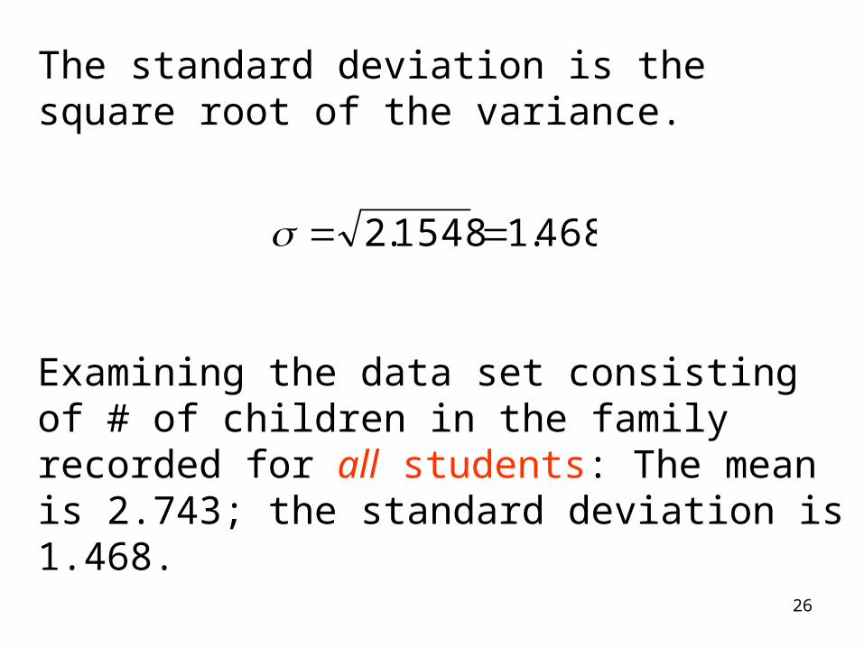
The standard deviation is the square root of the variance.
Examining the data set consisting of # of children in the family recorded for all students: The mean is 2.743; the standard deviation is 1.468.
468.11548.2
27
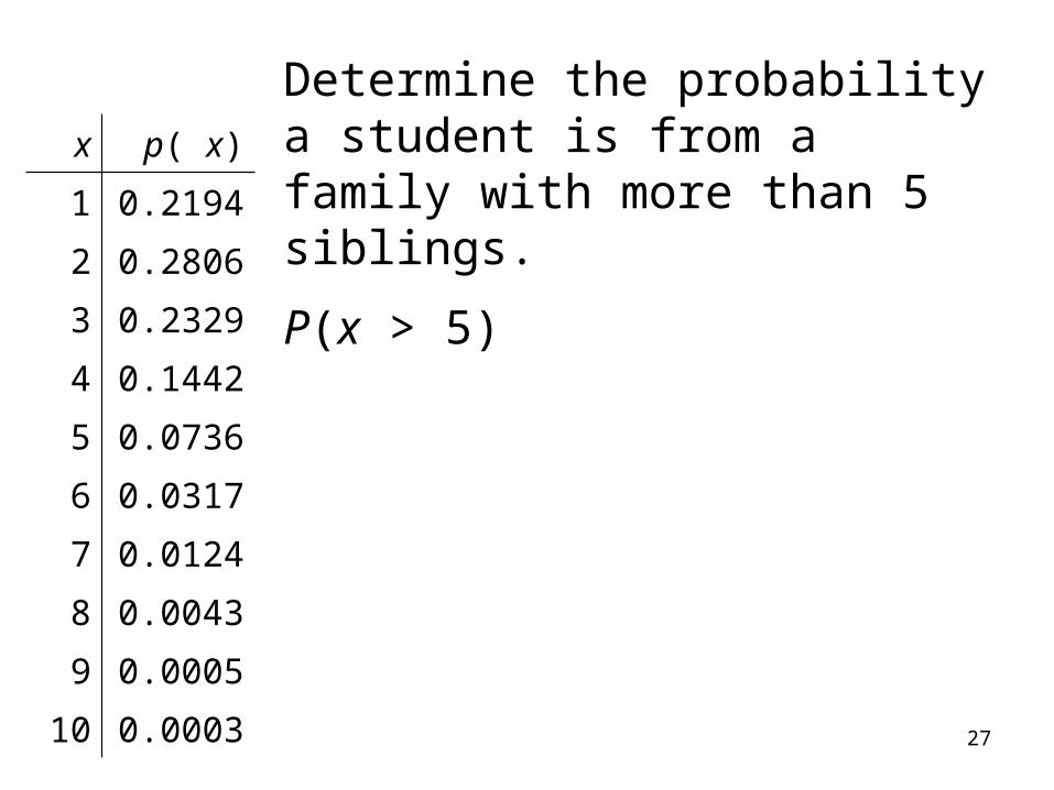
Determine the probability a student is from a family with more than 5 siblings.
P(x > 5)
x p( x)
1 0.2194
2 0.2806
3 0.2329
4 0.1442
5 0.0736
6 0.0317
7 0.0124
8 0.0043
9 0.0005
10 0.0003
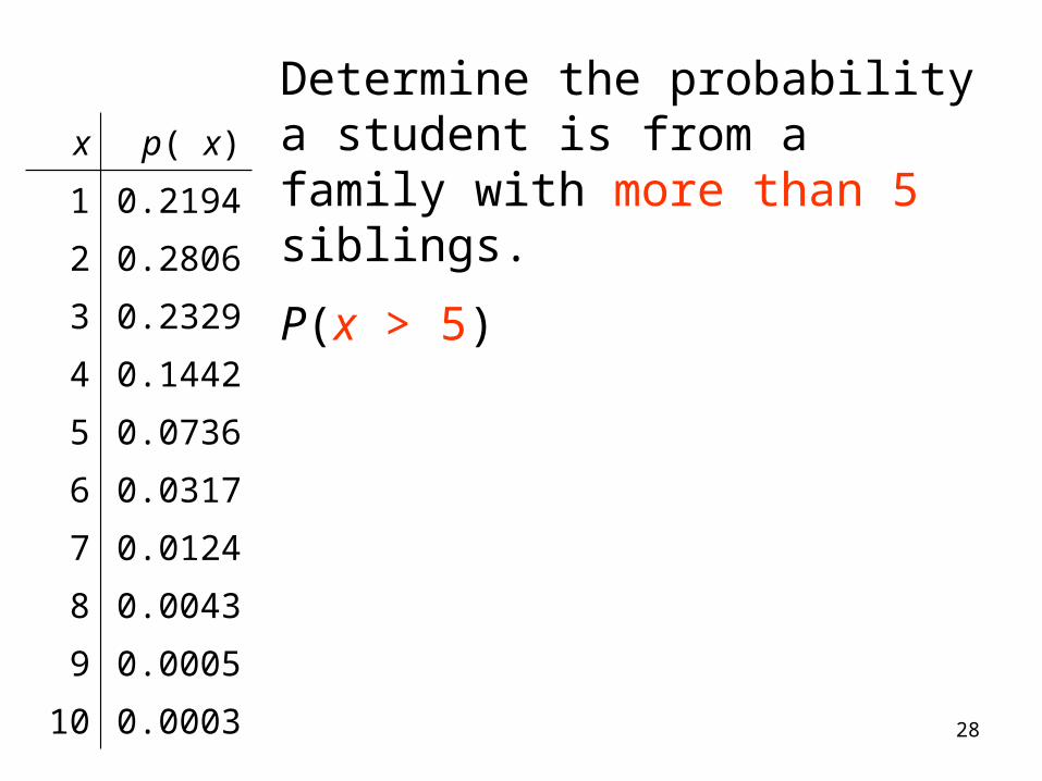
28
Determine the probability a student is from a family with more than 5 siblings.
P(x > 5)
x p( x)
1 0.2194
2 0.2806
3 0.2329
4 0.1442
5 0.0736
6 0.0317
7 0.0124
8 0.0043
9 0.0005
10 0.0003
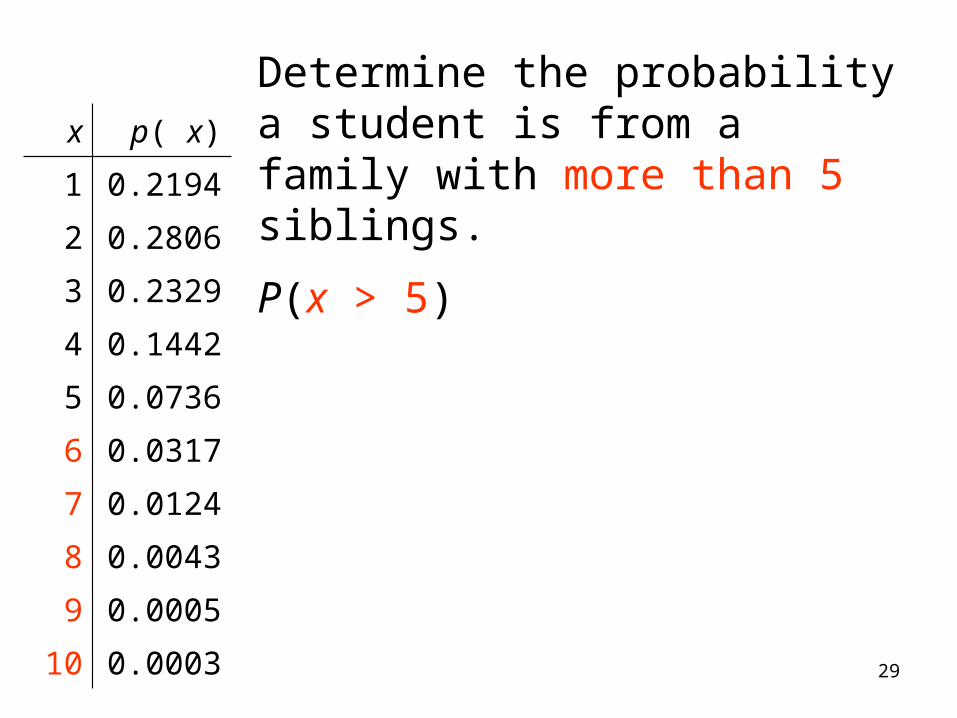
29
Determine the probability a student is from a family with more than 5 siblings.
P(x > 5)
x p( x)
1 0.2194
2 0.2806
3 0.2329
4 0.1442
5 0.0736
6 0.0317
7 0.0124
8 0.0043
9 0.0005
10 0.0003
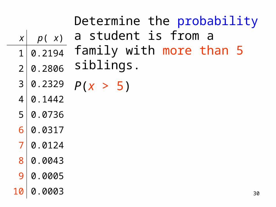
30
Determine the probability a student is from a family with more than 5 siblings.
P(x > 5)
x p( x)
1 0.2194
2 0.2806
3 0.2329
4 0.1442
5 0.0736
6 0.0317
7 0.0124
8 0.0043
9 0.0005
10 0.0003
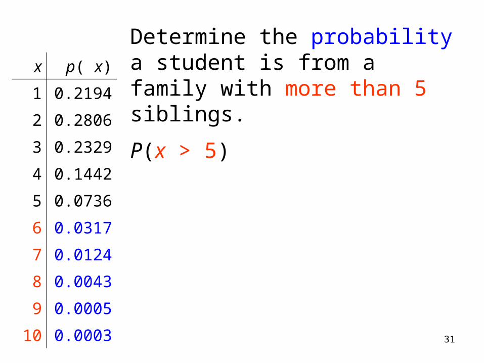
31
Determine the probability a student is from a family with more than 5 siblings.
P(x > 5)
x p( x)
1 0.2194
2 0.2806
3 0.2329
4 0.1442
5 0.0736
6 0.0317
7 0.0124
8 0.0043
9 0.0005
10 0.0003
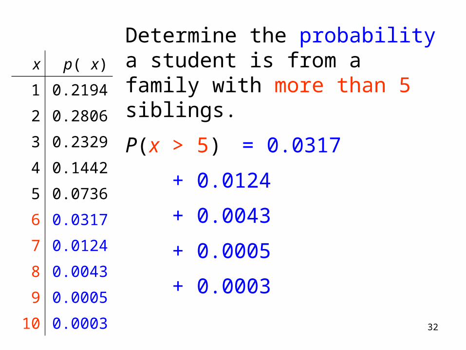
32
Determine the probability a student is from a family with more than 5 siblings.
P(x > 5) = 0.0317
+ 0.0124
+ 0.0043
+ 0.0005
+ 0.0003
x p( x)
1 0.2194
2 0.2806
3 0.2329
4 0.1442
5 0.0736
6 0.0317
7 0.0124
8 0.0043
9 0.0005
10 0.0003
33
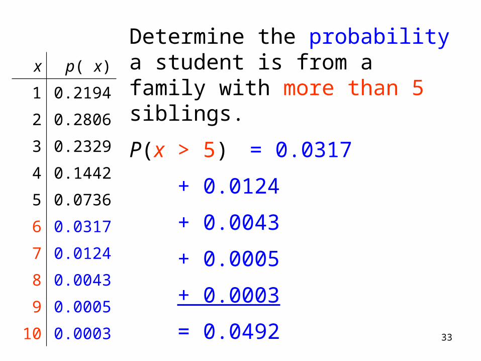
Determine the probability a student is from a family with more than 5 siblings.
P(x > 5) = 0.0317
+ 0.0124
+ 0.0043
+ 0.0005
+ 0.0003
= 0.0492
x p( x)
1 0.2194
2 0.2806
3 0.2329
4 0.1442
5 0.0736
6 0.0317
7 0.0124
8 0.0043
9 0.0005
10 0.0003

34
Determine the probability a student is from a family with more than 5 siblings.
P(x > 5) = 0.0492
4.92% of all college students come from families with more than 5 children (they have 4 or more brothers and sisters).
x p( x)
1 0.2194
2 0.2806
3 0.2329
4 0.1442
5 0.0736
6 0.0317
7 0.0124
8 0.0043
9 0.0005
10 0.0003
35
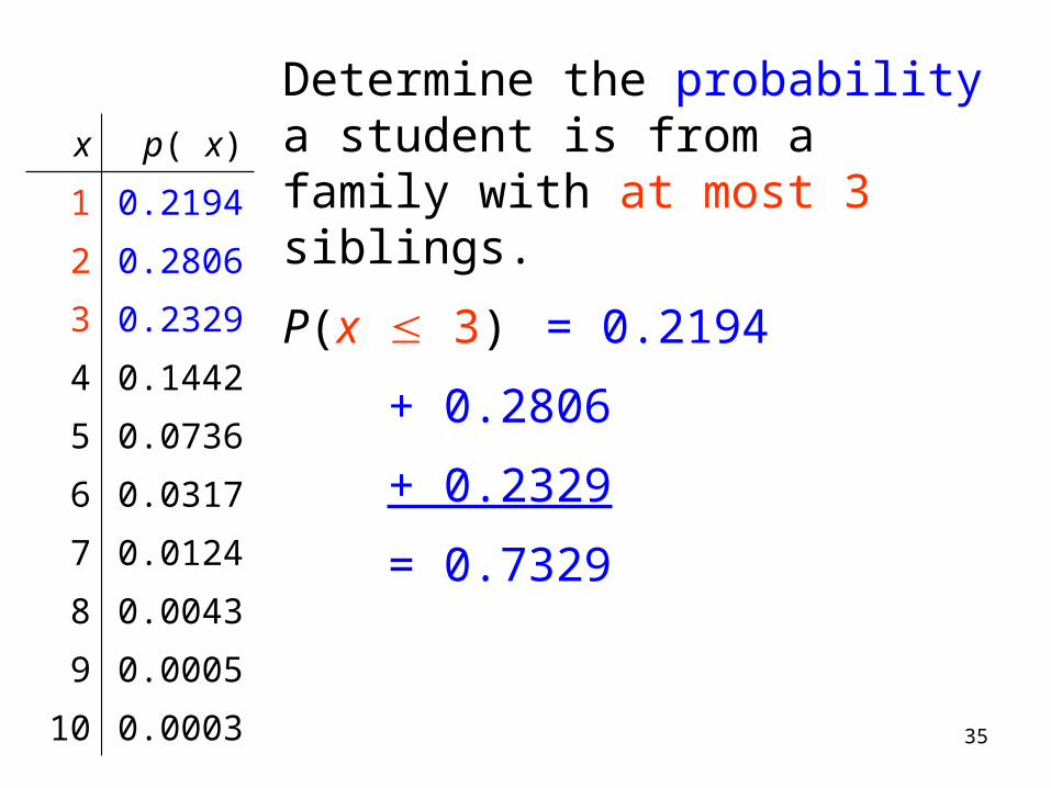
Determine the probability a student is from a family with at most 3 siblings.
P(x 3) = 0.2194
+ 0.2806
+ 0.2329
= 0.7329
x p( x)
1 0.2194
2 0.2806
3 0.2329
4 0.1442
5 0.0736
6 0.0317
7 0.0124
8 0.0043
9 0.0005
10 0.0003
36
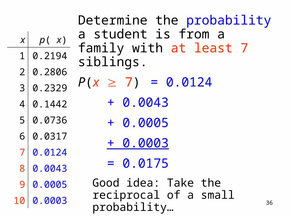
Determine the probability a student is from a family with at least 7 siblings.
P(x 7) = 0.0124
+ 0.0043
+ 0.0005
+ 0.0003
= 0.0175
Good idea: Take the reciprocal of a small probability…
1/.0175 = 57.1 1 in 57 students
x p( x)
1 0.2194
2 0.2806
3 0.2329
4 0.1442
5 0.0736
6 0.0317
7 0.0124
8 0.0043
9 0.0005
10 0.0003
37
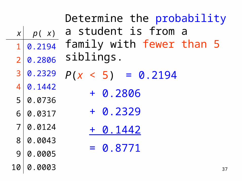
Determine the probability a student is from a family with fewer than 5 siblings.
P(x < 5) = 0.2194
+ 0.2806
+ 0.2329
+ 0.1442
= 0.8771
x p( x)
1 0.2194
2 0.2806
3 0.2329
4 0.1442
5 0.0736
6 0.0317
7 0.0124
8 0.0043
9 0.0005
10 0.0003
38
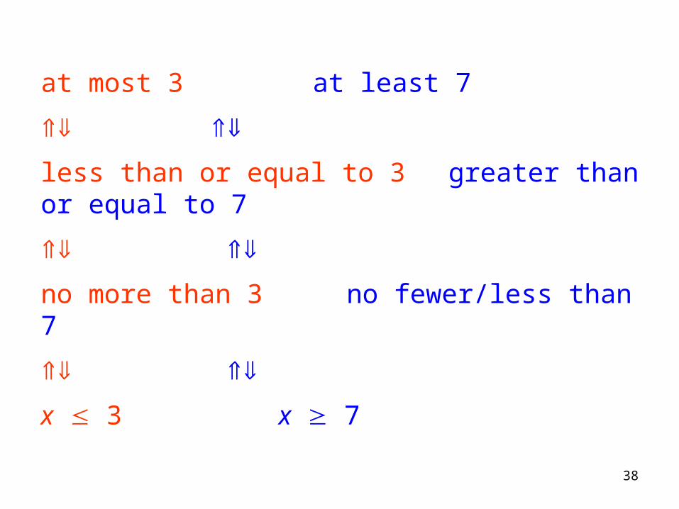
at most 3 at least 7
less than or equal to 3 greater than or equal to 7
no more than 3 no fewer/less than 7
x 3 x 7
39
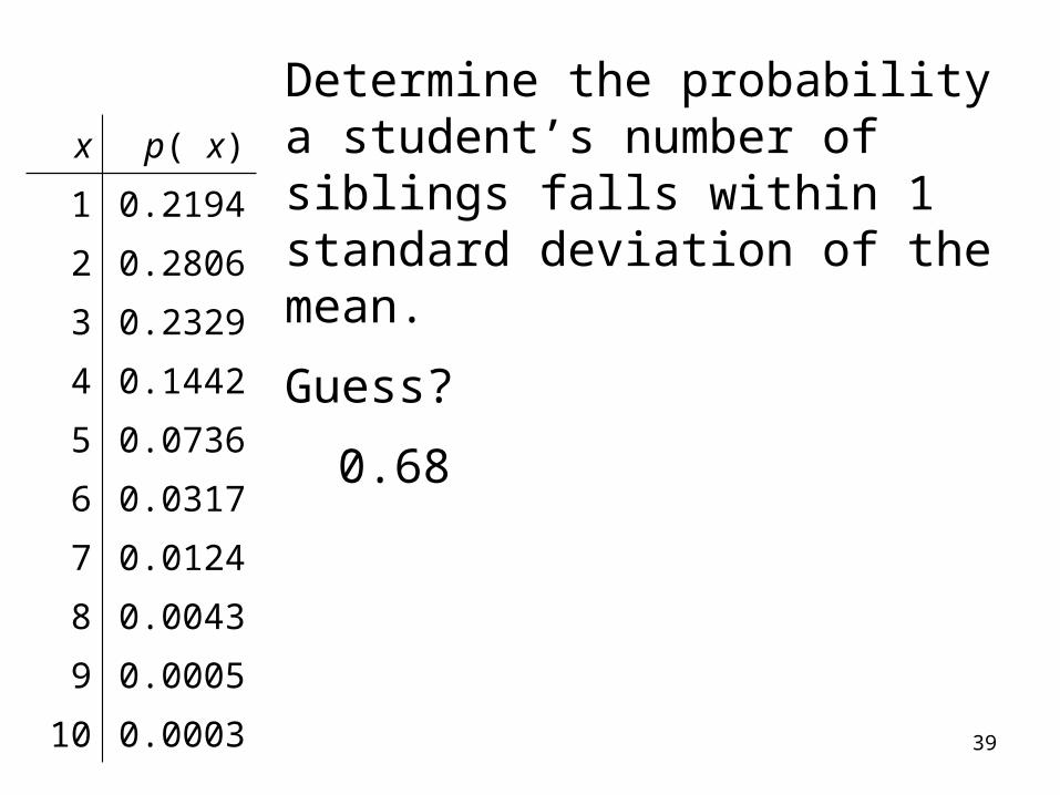
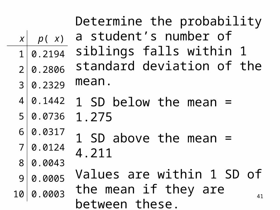
Determine the probability a student’s number of siblings falls within 1 standard deviation of the mean.
Guess?
0.68
x p( x)
1 0.2194
2 0.2806
3 0.2329
4 0.1442
5 0.0736
6 0.0317
7 0.0124
8 0.0043
9 0.0005
10 0.0003
40
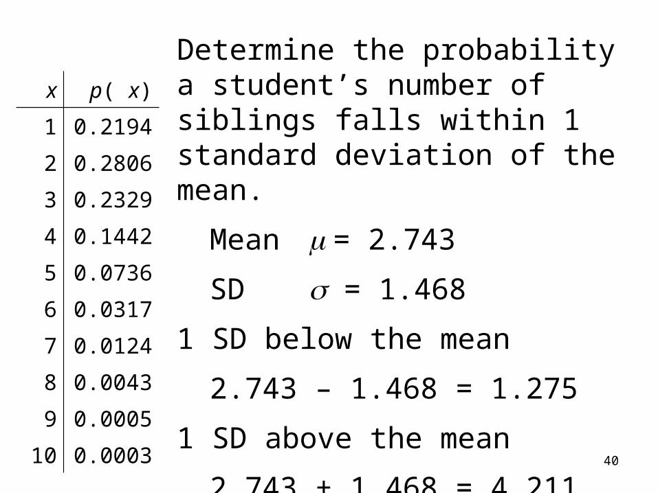
Determine the probability a student’s number of siblings falls within 1 standard deviation of the mean.
Mean = 2.743
SD = 1.468
1 SD below the mean
2.743 – 1.468 = 1.275
1 SD above the mean
2.743 + 1.468 = 4.211
x p( x)
1 0.2194
2 0.2806
3 0.2329
4 0.1442
5 0.0736
6 0.0317
7 0.0124
8 0.0043
9 0.0005
10 0.0003
41
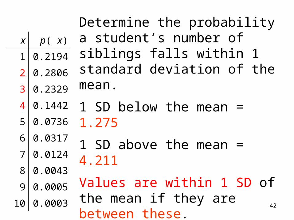
Determine the probability a student’s number of siblings falls within 1 standard deviation of the mean.
1 SD below the mean = 1.275
1 SD above the mean = 4.211
Values are within 1 SD of the mean if they are between these.
x p( x)
1 0.2194
2 0.2806
3 0.2329
4 0.1442
5 0.0736
6 0.0317
7 0.0124
8 0.0043
9 0.0005
10 0.0003
42
Determine the probability a student’s number of siblings falls within 1 standard deviation of the mean.
1 SD below the mean = 1.275
1 SD above the mean = 4.211
Values are within 1 SD of the mean if they are between these.
x p( x)
1 0.2194
2 0.2806
3 0.2329
4 0.1442
5 0.0736
6 0.0317
7 0.0124
8 0.0043
9 0.0005
10 0.0003
43
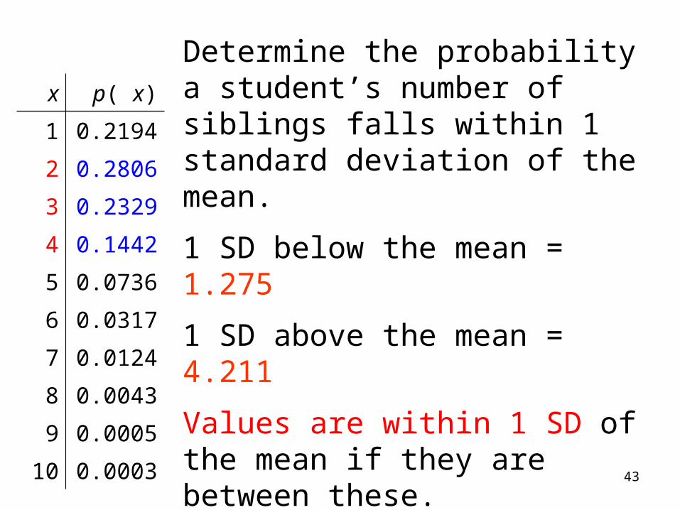
Determine the probability a student’s number of siblings falls within 1 standard deviation of the mean.
1 SD below the mean = 1.275
1 SD above the mean = 4.211
Values are within 1 SD of the mean if they are between these.
The probability of being between these:
0.2806 + 0.2329 + 0.1442 = 0.6577
x p( x)
1 0.2194
2 0.2806
3 0.2329
4 0.1442
5 0.0736
6 0.0317
7 0.0124
8 0.0043
9 0.0005
10 0.0003
44
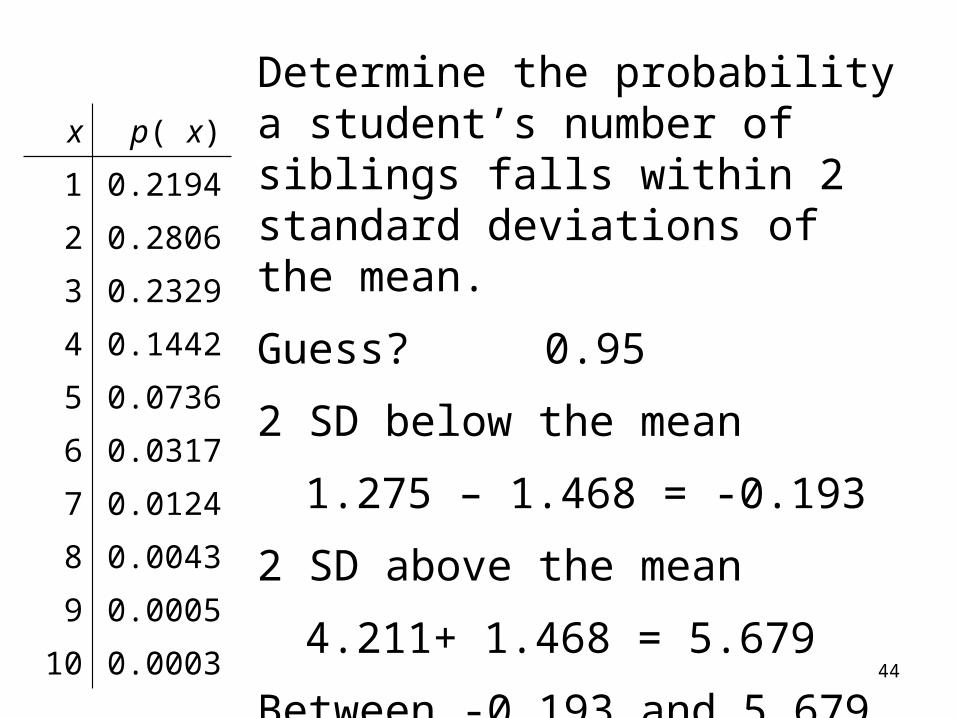
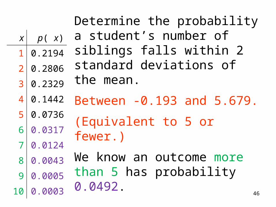
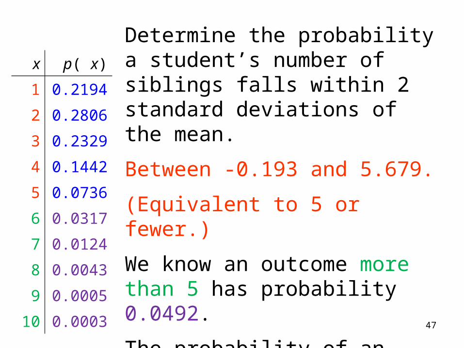
Determine the probability a student’s number of siblings falls within 2 standard deviations of the mean.
Guess? 0.95
2 SD below the mean
1.275 – 1.468 = -0.193
2 SD above the mean
4.211+ 1.468 = 5.679
Between -0.193 and 5.679.
x p( x)
1 0.2194
2 0.2806
3 0.2329
4 0.1442
5 0.0736
6 0.0317
7 0.0124
8 0.0043
9 0.0005
10 0.0003
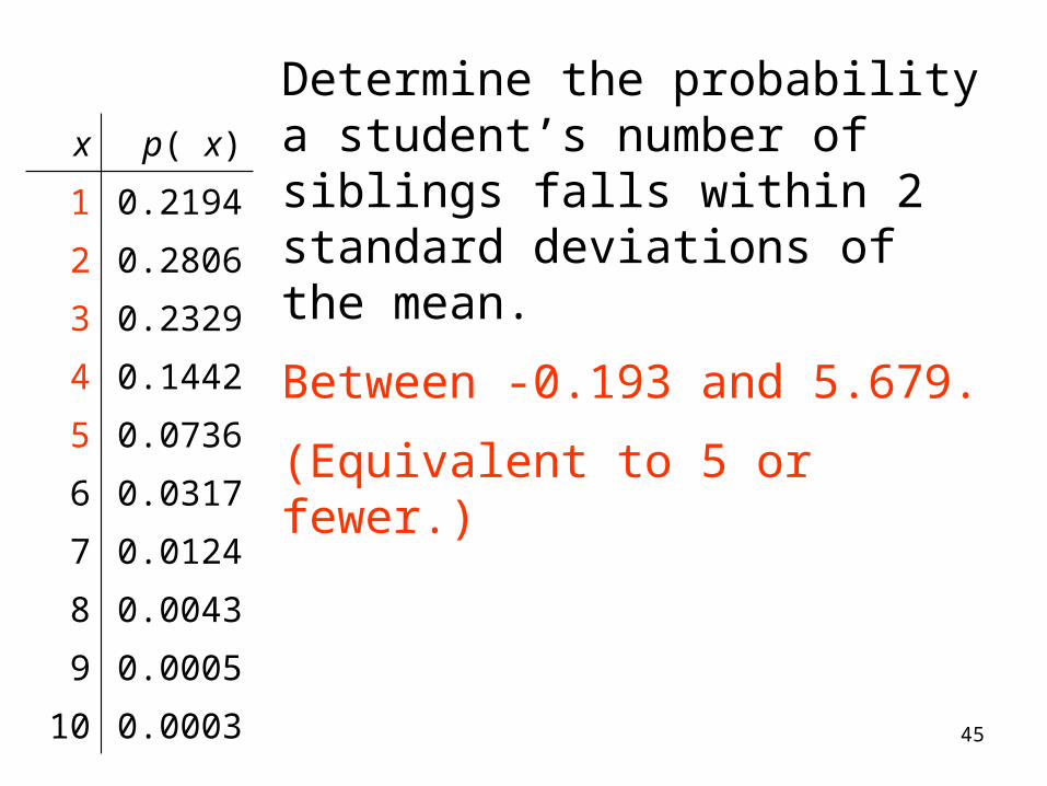
45
Determine the probability a student’s number of siblings falls within 2 standard deviations of the mean.
Between -0.193 and 5.679.
(Equivalent to 5 or fewer.)
x p( x)
1 0.2194
2 0.2806
3 0.2329
4 0.1442
5 0.0736
6 0.0317
7 0.0124
8 0.0043
9 0.0005
10 0.0003
46
Determine the probability a student’s number of siblings falls within 2 standard deviations of the mean.
Between -0.193 and 5.679.
(Equivalent to 5 or fewer.)
We know an outcome more than 5 has probability 0.0492.
x p( x)
1 0.2194
2 0.2806
3 0.2329
4 0.1442
5 0.0736
6 0.0317
7 0.0124
8 0.0043
9 0.0005
10 0.0003
47
Determine the probability a student’s number of siblings falls within 2 standard deviations of the mean.
Between -0.193 and 5.679.
(Equivalent to 5 or fewer.)
We know an outcome more than 5 has probability 0.0492.
The probability of an outcome at most 5 is 1 – 0.0492 = 0.9508.
x p( x)
1 0.2194
2 0.2806
3 0.2329
4 0.1442
5 0.0736
6 0.0317
7 0.0124
8 0.0043
9 0.0005
10 0.0003

48
Determine the probability a student’s number of siblings falls within 2 standard deviations of the mean.
Between -0.193 and 5.679.
0.9508.
x p( x)
1 0.2194
2 0.2806
3 0.2329
4 0.1442
5 0.0736
6 0.0317
7 0.0124
8 0.0043
9 0.0005
10 0.0003
49
A company monitors pollutants downstream of discharge into a stream.
Data were collected on 200 days from a point 1 mile downstream of the plant on Stream A.
Data were collected on 100 days from a point 1 miles downstream of the plant on Stream B.
Pollutant Particles in Streamwater
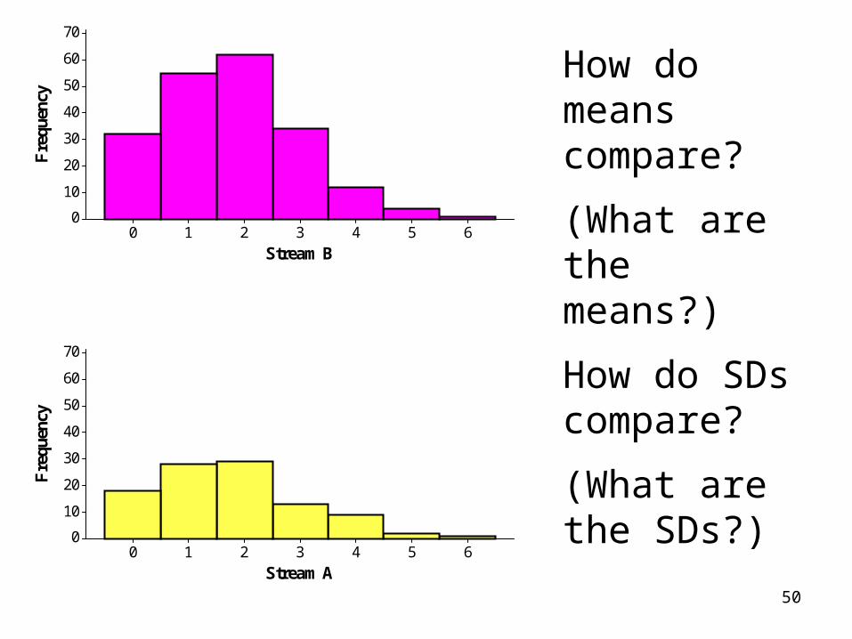
50
How do means compare?
(What are the means?)
How do SDs compare?
(What are the SDs?)
6543210
70
60
50
40
30
20
10
0
Stream A
Fre
quen
cy
6543210
70
60
50
40
30
20
10
0
Stream B
Fre
quen
cy
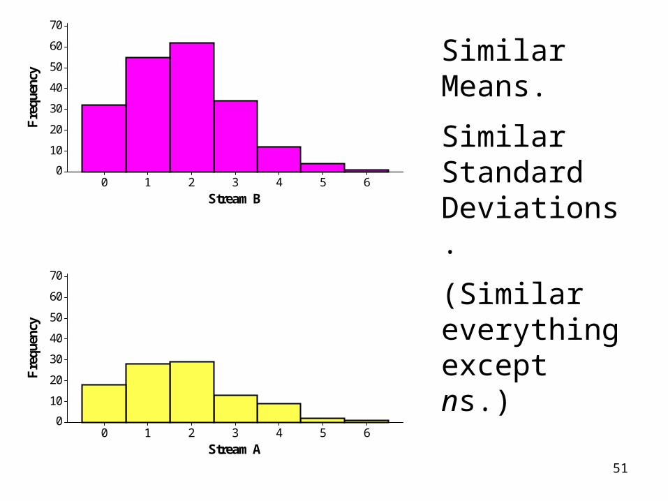
51
Similar Means.
Similar Standard Deviations.
(Similar everything except ns.)
6543210
70
60
50
40
30
20
10
0
Stream A
Fre
quen
cy
6543210
70
60
50
40
30
20
10
0
Stream B
Fre
quen
cy
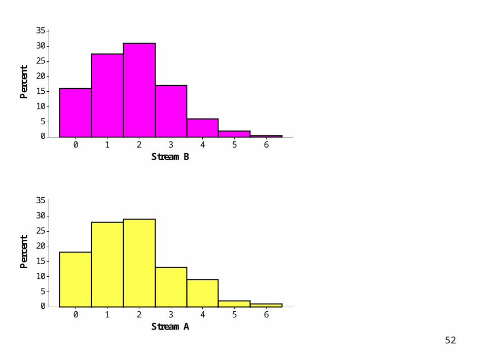
52
6543210
35
30
25
20
15
10
5
0
Stream A
Per
cent
6543210
35
30
25
20
15
10
5
0
Stream B
Per
cent
53
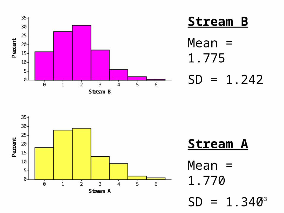
Stream B
Mean = 1.775
SD = 1.242
Stream A
Mean = 1.770
SD = 1.3406543210
35
30
25
20
15
10
5
0
Stream A
Per
cent
6543210
35
30
25
20
15
10
5
0
Stream B
Per
cent
54
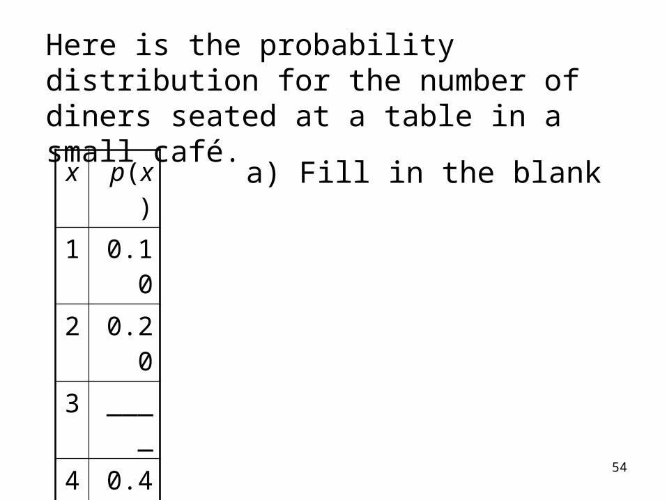
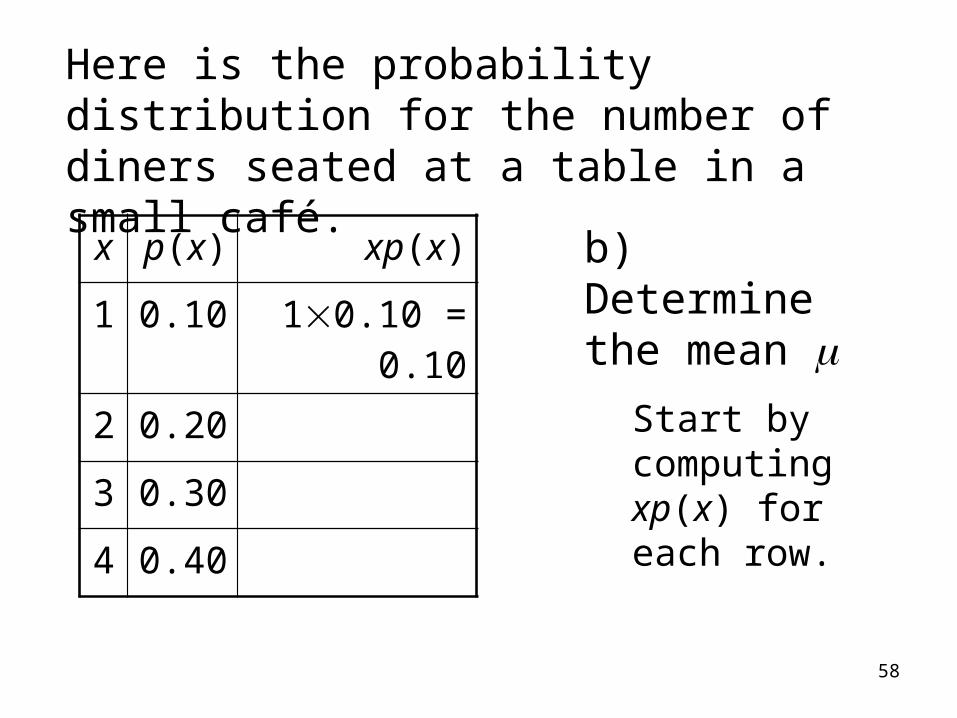
Here is the probability distribution for the number of diners seated at a table in a small café.
x p(x)
1 0.10
2 0.20
3 ____
4 0.40
a) Fill in the blank
55
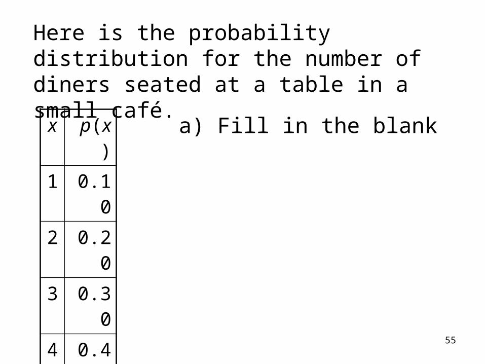
x p(x)
1 0.10
2 0.20
3 0.30
4 0.40
a) Fill in the blank
Here is the probability distribution for the number of diners seated at a table in a small café.
56
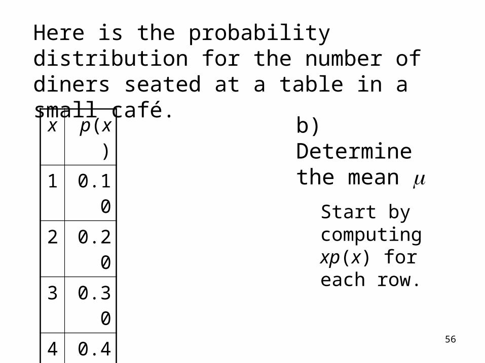
b) Determine the mean
Start by computing xp(x) for each row.
x p(x)
1 0.10
2 0.20
3 0.30
4 0.40
Here is the probability distribution for the number of diners seated at a table in a small café.
57
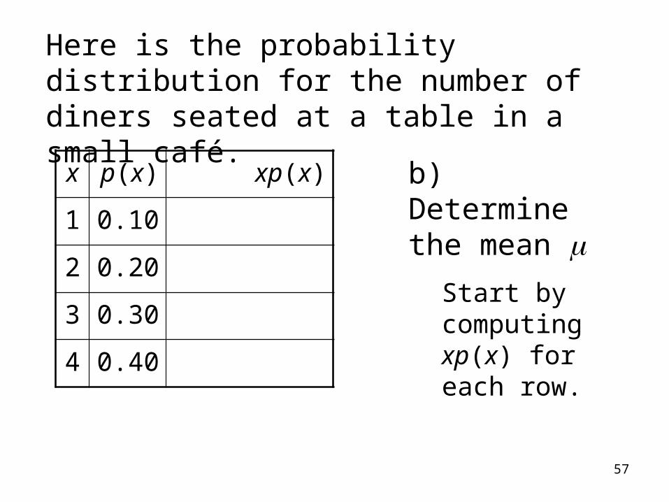
x p(x) xp(x)
1 0.10
2 0.20
3 0.30
4 0.40
b) Determine the mean
Start by computing xp(x) for each row.
Here is the probability distribution for the number of diners seated at a table in a small café.
58
x p(x) xp(x)
1 0.10 10.10 = 0.10
2 0.20
3 0.30
4 0.40
b) Determine the mean
Start by computing xp(x) for each row.
Here is the probability distribution for the number of diners seated at a table in a small café.
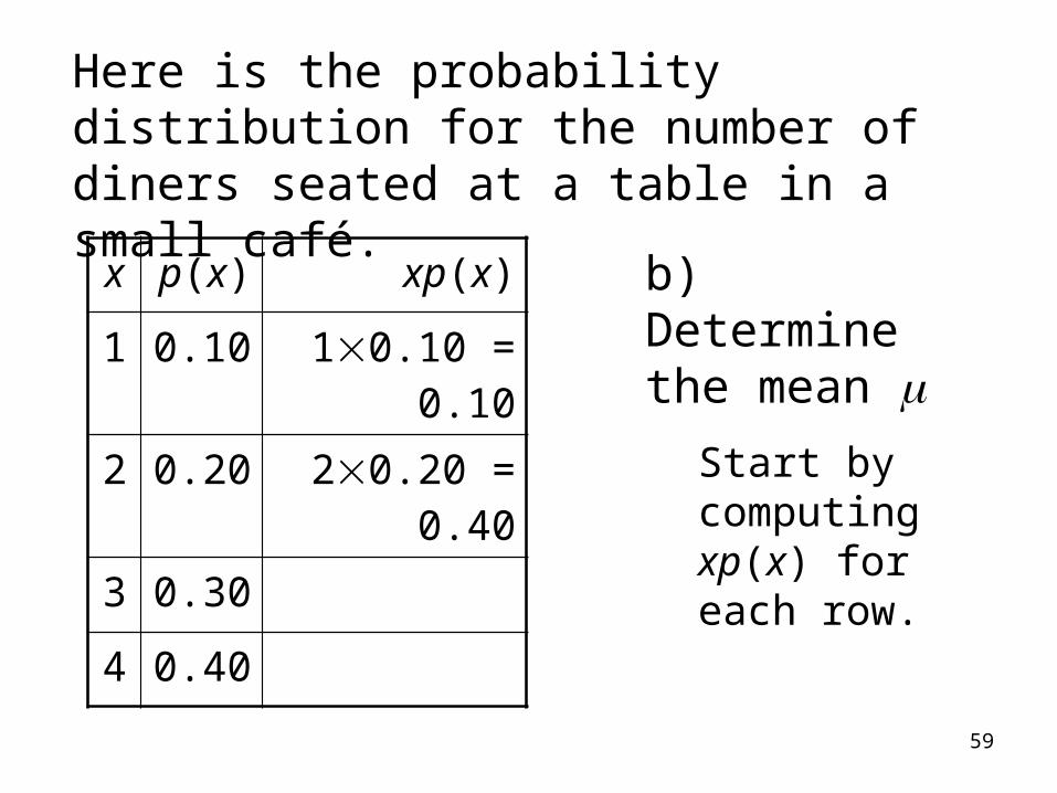
59
x p(x) xp(x)
1 0.10 10.10 = 0.10
2 0.20 20.20 = 0.40
3 0.30
4 0.40
b) Determine the mean
Start by computing xp(x) for each row.
Here is the probability distribution for the number of diners seated at a table in a small café.
60
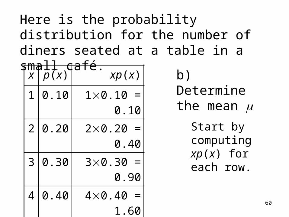
x p(x) xp(x)
1 0.10 10.10 = 0.10
2 0.20 20.20 = 0.40
3 0.30 30.30 = 0.90
4 0.40 40.40 = 1.60
b) Determine the mean
Start by computing xp(x) for each row.
Here is the probability distribution for the number of diners seated at a table in a small café.
61
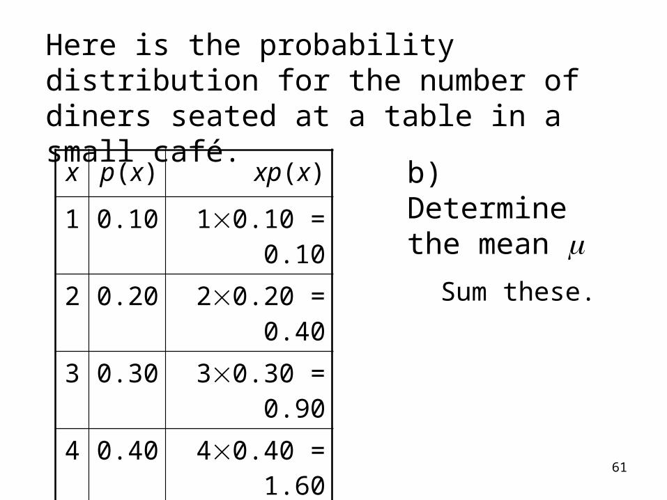
x p(x) xp(x)
1 0.10 10.10 = 0.10
2 0.20 20.20 = 0.40
3 0.30 30.30 = 0.90
4 0.40 40.40 = 1.60
b) Determine the mean
Sum these.
Here is the probability distribution for the number of diners seated at a table in a small café.
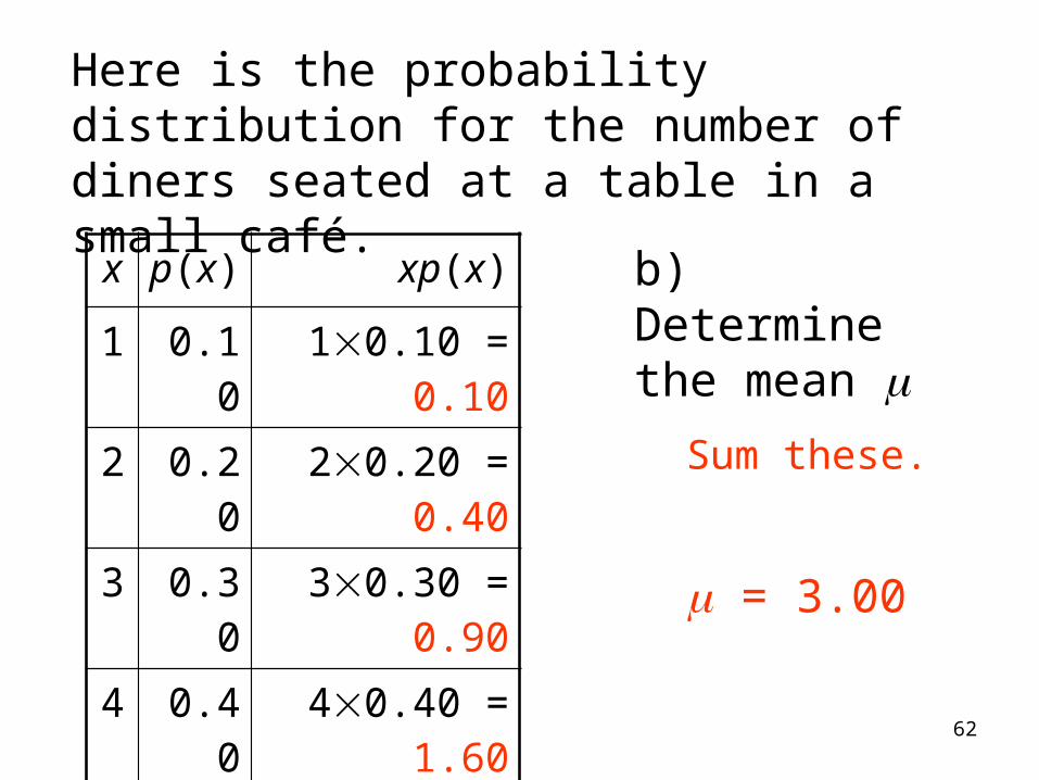
62
x p(x) xp(x)
1 0.10 10.10 = 0.10
2 0.20 20.20 = 0.40
3 0.30 30.30 = 0.90
4 0.40 40.40 = 1.60
b) Determine the mean
Sum these.
= 3.00
Here is the probability distribution for the number of diners seated at a table in a small café.

63
b) Determine the standard deviation
Start by computing
( x – ) 2 p(x)
for each row.
x p(x)
1 0.10
2 0.20
3 0.30
4 0.40
Here is the probability distribution for the number of diners seated at a table in a small café.
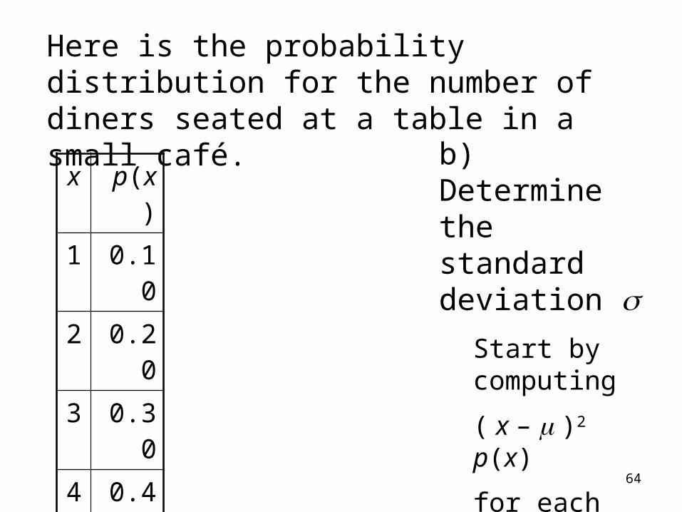
64
b) Determine the standard deviation
Start by computing
( x – )2 p(x)
for each row.
= 3
x p(x)
1 0.10
2 0.20
3 0.30
4 0.40
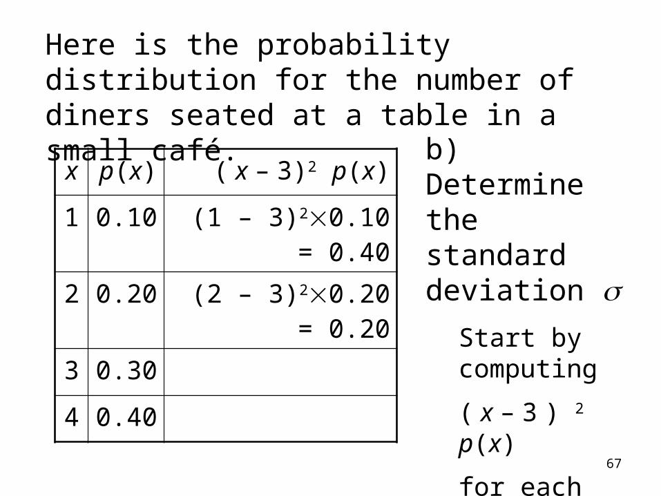
Here is the probability distribution for the number of diners seated at a table in a small café.
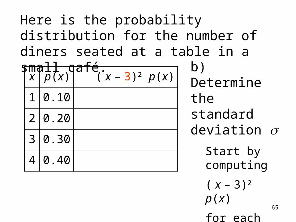
65
x p(x) ( x – 3)2 p(x)
1 0.10
2 0.20
3 0.30
4 0.40
b) Determine the standard deviation
Start by computing
( x – 3)2 p(x)
for each row.
= 3
Here is the probability distribution for the number of diners seated at a table in a small café.
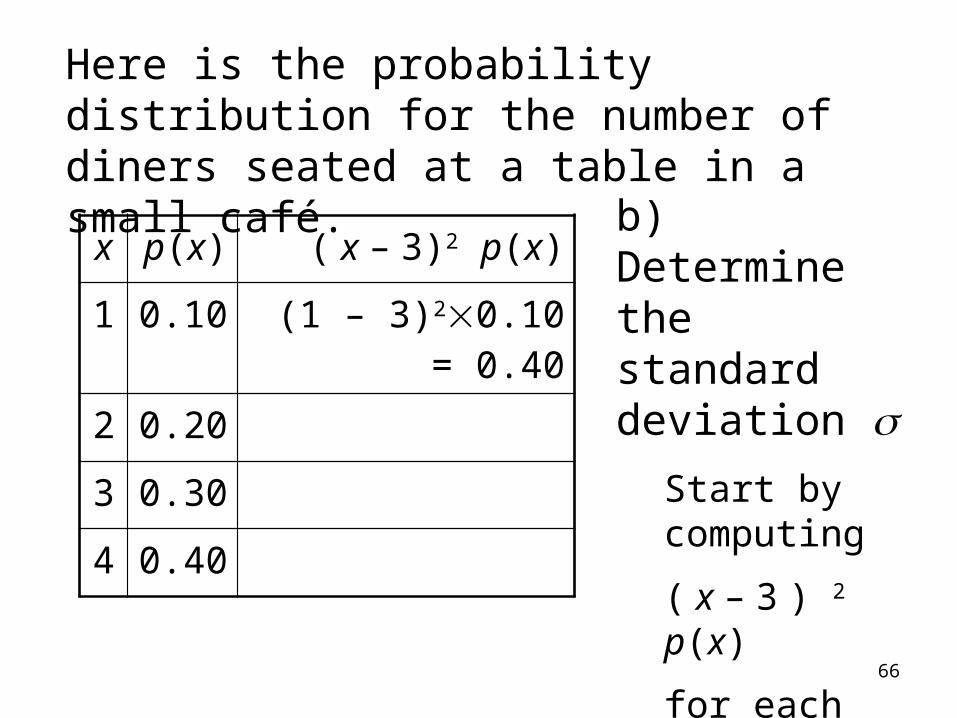
66
x p(x) ( x – 3)2 p(x)
1 0.10 (1 – 3)20.10 = 0.40
2 0.20
3 0.30
4 0.40
b) Determine the standard deviation
Start by computing
( x – 3 ) 2 p(x)
for each row.
= 3
Here is the probability distribution for the number of diners seated at a table in a small café.
67
x p(x) ( x – 3)2 p(x)
1 0.10 (1 – 3)20.10 = 0.40
2 0.20 (2 – 3)20.20 = 0.20
3 0.30
4 0.40
b) Determine the standard deviation
Start by computing
( x – 3 ) 2 p(x)
for each row.
= 3
Here is the probability distribution for the number of diners seated at a table in a small café.
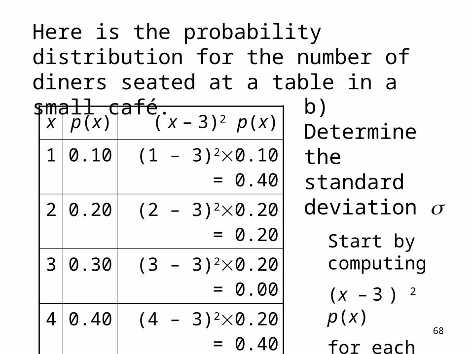
68
x p(x) ( x – 3)2 p(x)
1 0.10 (1 – 3)20.10 = 0.40
2 0.20 (2 – 3)20.20 = 0.20
3 0.30 (3 – 3)20.20 = 0.00
4 0.40 (4 – 3)20.20 = 0.40
b) Determine the standard deviation
Start by computing
(x – 3 ) 2 p(x)
for each row.
= 3
Here is the probability distribution for the number of diners seated at a table in a small café.
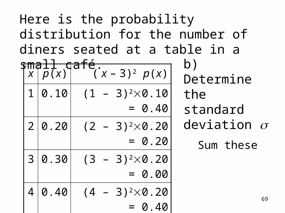
69
x p(x) ( x – 3)2 p(x)
1 0.10 (1 – 3)20.10 = 0.40
2 0.20 (2 – 3)20.20 = 0.20
3 0.30 (3 – 3)20.20 = 0.00
4 0.40 (4 – 3)20.20 = 0.40
b) Determine the standard deviation
Sum these
Here is the probability distribution for the number of diners seated at a table in a small café.
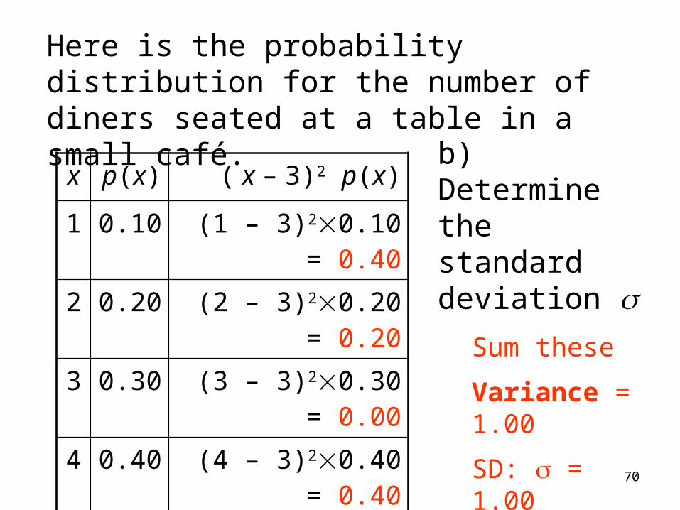
70
x p(x) ( x – 3)2 p(x)
1 0.10 (1 – 3)20.10 = 0.40
2 0.20 (2 – 3)20.20 = 0.20
3 0.30 (3 – 3)20.30 = 0.00
4 0.40 (4 – 3)20.40 = 0.40
b) Determine the standard deviation
Sum these
Variance = 1.00
SD: = 1.00
Here is the probability distribution for the number of diners seated at a table in a small café.

71
This framework makes it possible to obtain fairly good approximations to means and standard deviations from a histogram of continuous data.
[Optional] Application
72
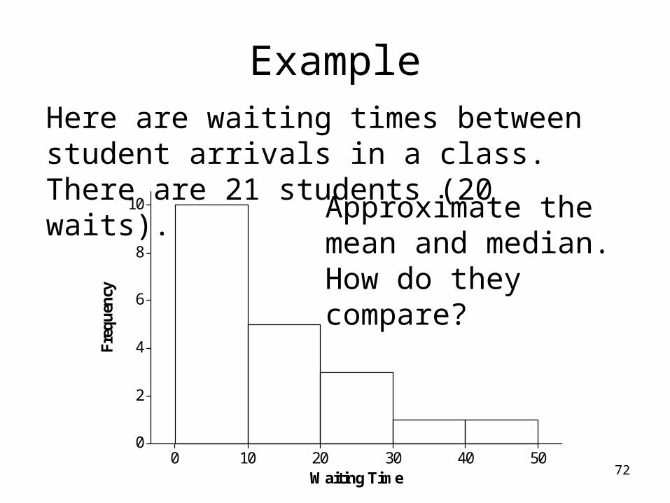
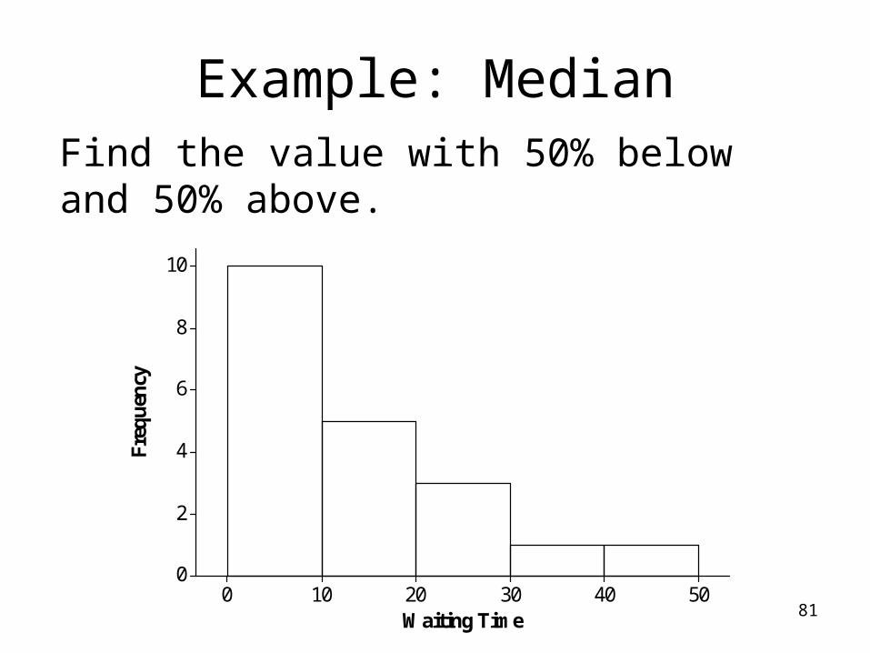
Here are waiting times between student arrivals in a class. There are 21 students (20 waits).
Example
50403020100
10
8
6
4
2
0
Waiting Time
Freq
uen
cy
Approximate the mean and median. How do they compare?
7350403020100
10
8
6
4
2
0
Waiting Time
Freq
uen
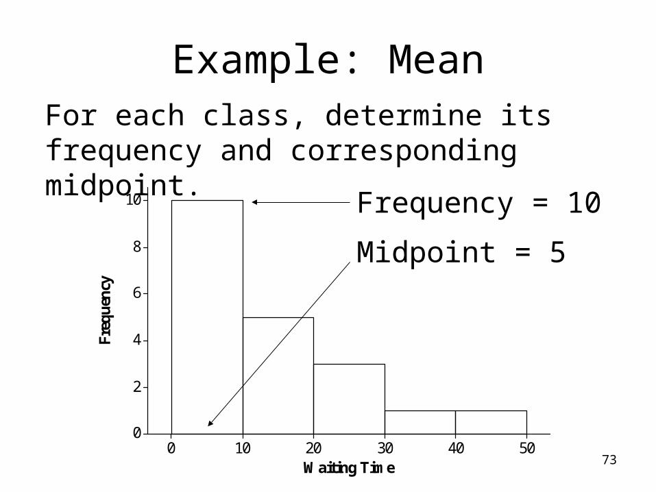
cyFor each class, determine its frequency and corresponding midpoint.
Example: Mean
Frequency = 10
Midpoint = 5
74
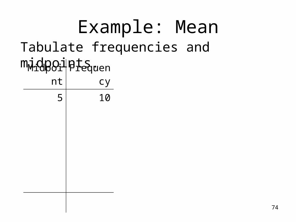
Tabulate frequencies and midpoints.
Example: Mean
Midpoint
Frequency
5 10
75
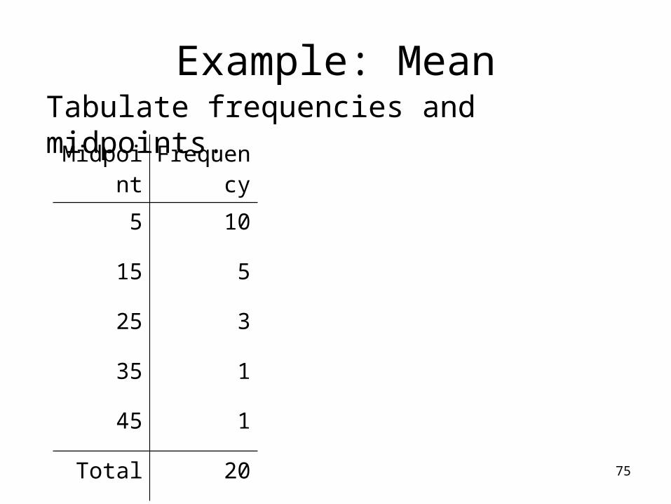
Tabulate frequencies and midpoints.
Example: Mean
Midpoint
Frequency
5 10
15 5
25 3
35 1
45 1
Total 20
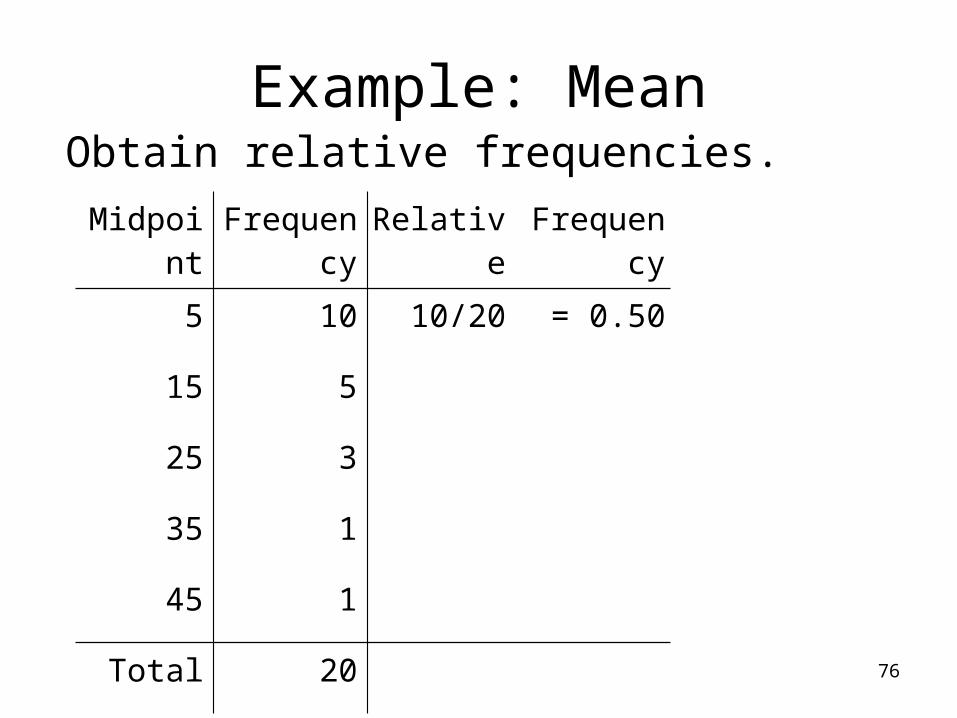
76
Obtain relative frequencies.
Example: Mean
Midpoint
Frequency
Relative Frequency
5 10 10/20 = 0.50
15 5
25 3
35 1
45 1
Total 20
77
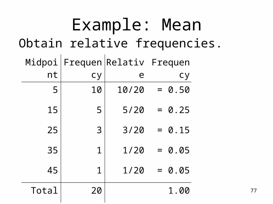
Obtain relative frequencies.
Example: Mean
Midpoint
Frequency
Relative Frequency
5 10 10/20 = 0.50
15 5 5/20 = 0.25
25 3 3/20 = 0.15
35 1 1/20 = 0.05
45 1 1/20 = 0.05
Total 20 1.00
78
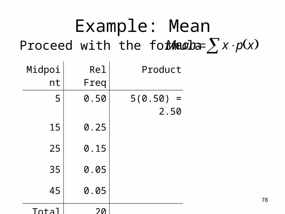
Proceed with the formula
Example: Mean
Midpoint
Rel Freq Product
5 0.50 5(0.50) = 2.50
15 0.25
25 0.15
35 0.05
45 0.05
Total 20
xpxMean
79
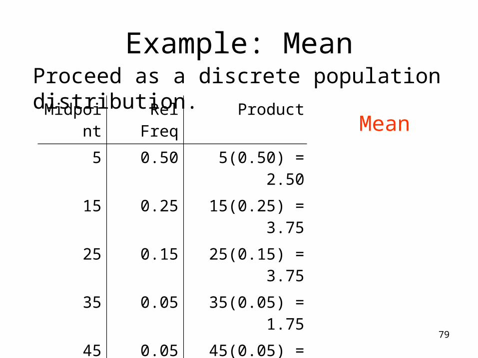
Proceed as a discrete population distribution.
Example: Mean
Midpoint
Rel Freq Product
5 0.50 5(0.50) = 2.50
15 0.25 15(0.25) = 3.75
25 0.15 25(0.15) = 3.75
35 0.05 35(0.05) = 1.75
45 0.05 45(0.05) = 2.25
Total 20
Mean
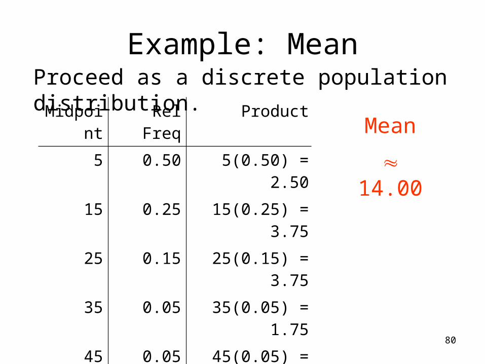
80
Proceed as a discrete population distribution.
Example: Mean
Midpoint
Rel Freq Product
5 0.50 5(0.50) = 2.50
15 0.25 15(0.25) = 3.75
25 0.15 25(0.15) = 3.75
35 0.05 35(0.05) = 1.75
45 0.05 45(0.05) = 2.25
Total 20 14.00
Mean
14.00
8150403020100
10
8
6
4
2
0
Waiting Time
Freq
uen
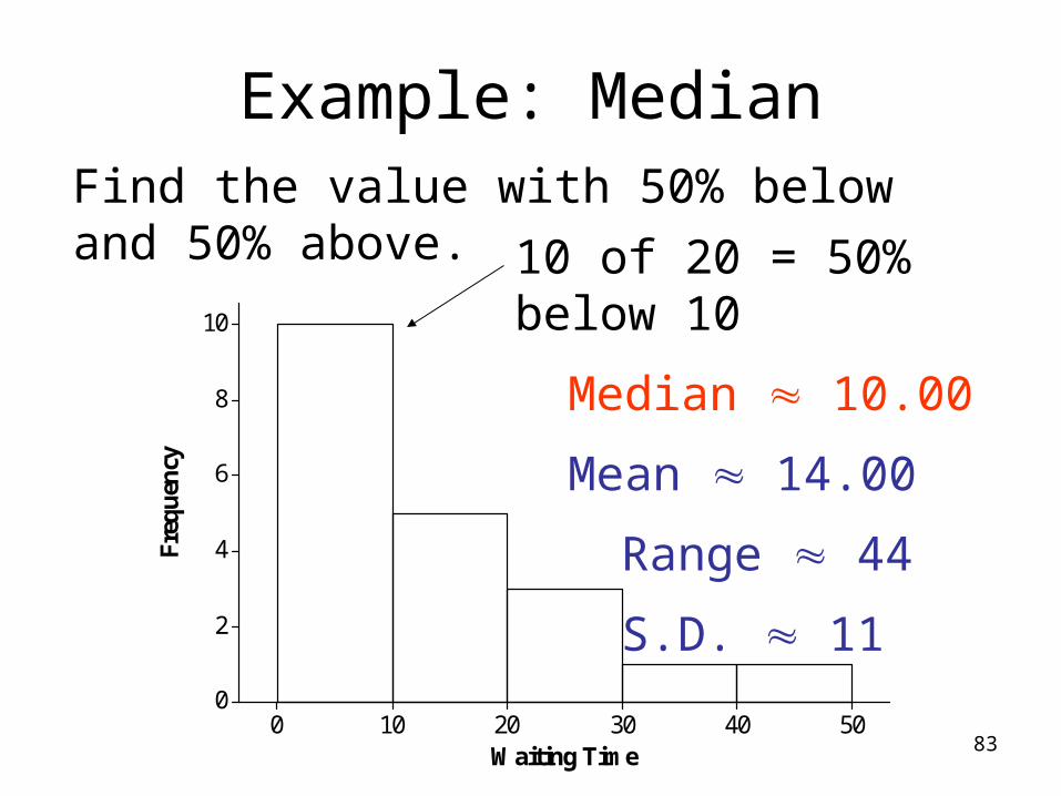
cyFind the value with 50% below and 50% above.
Example: Median
82
Obtain relative frequencies.
Example: Median
Midpoint
Rel Freq
5 0.50
15 0.20
25 0.15
35 0.05
45 0.05
Total 1.00
8350403020100
10
8
6
4
2
0
Waiting Time
Freq
uen
cyFind the value with 50% below and 50% above.
Example: Median
10 of 20 = 50% below 10
Median 10.00
Mean 14.00
Range 44
S.D. 11
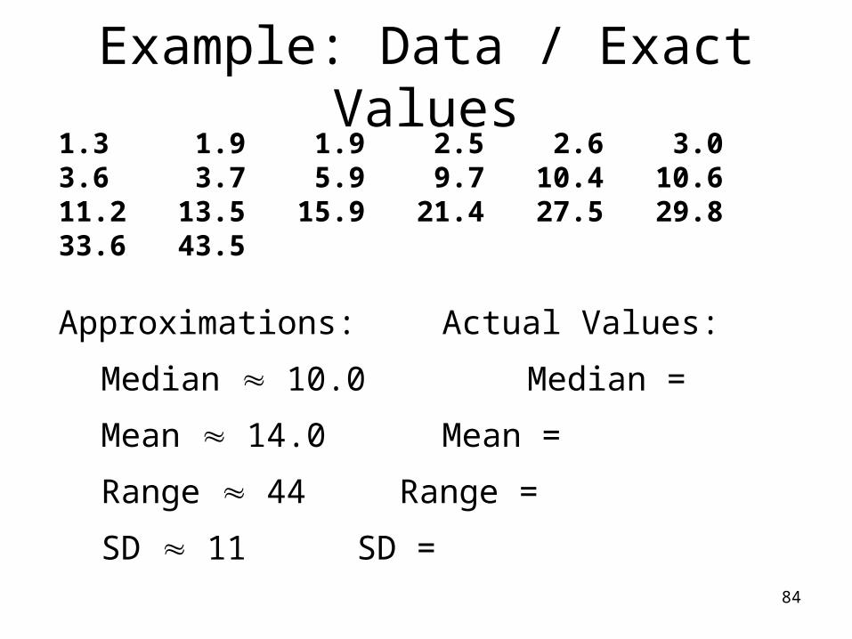
84
1.3 1.9 1.9 2.5 2.6 3.0 3.6 3.7 5.9 9.7 10.4 10.6 11.2 13.5 15.9 21.4 27.5 29.8 33.6 43.5
Approximations: Actual Values:
Median 10.0.05 Median =
Mean 14.0 Mean =
Range 44 Range =
SD 11 SD =
Example: Data / Exact Values
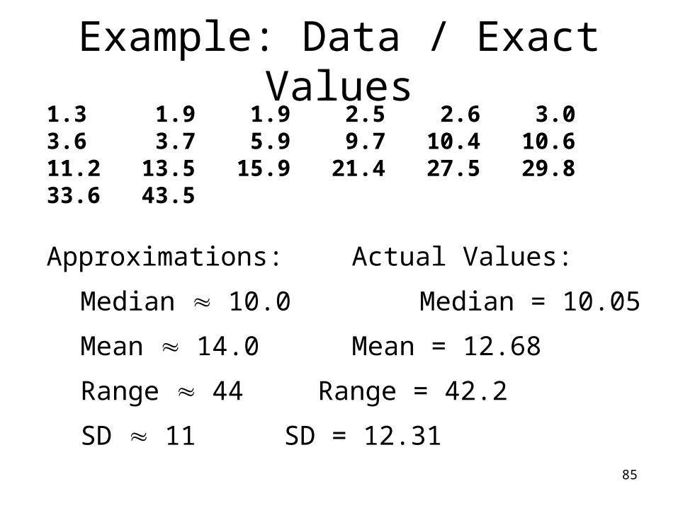
85
1.3 1.9 1.9 2.5 2.6 3.0 3.6 3.7 5.9 9.7 10.4 10.6 11.2 13.5 15.9 21.4 27.5 29.8 33.6 43.5
Approximations: Actual Values:
Median 10.0.05 Median = 10.05
Mean 14.0 Mean = 12.68
Range 44 Range = 42.2
SD 11 SD = 12.31
Example: Data / Exact Values