1 Path Loss Exponent Estimation in Large Wireless …mhaenggi/pubs/tsp08.pdf1 Path Loss Exponent...

1

Path Loss Exponent Estimation

in Large Wireless Networks

Sunil Srinivasa* and Martin Haenggi

Department of Electrical Engineering

University of Notre Dame

Notre Dame, IN 46556, USA

Email: {ssriniv1, mhaenggi}@nd.edu

Phone: (949) 331-7136, (574) 631-6103

Fax: (574) 631-4393

Abstract

Even though the analyses in many wireless networking problems assume that the value of the path

loss exponent (PLE) is known a priori, this is often not the case, and an accurate estimate is crucial

for the study and design of wireless systems. In this paper, we address the problem of estimating the

PLE in large wireless networks, which is relevant to severalimportant issues in communications such

as localization, energy-efficient routing, and channel access. We consider a large ad hoc network where

nodes are distributed as a homogeneous Poisson point process on the plane, and the channels are subject

to Nakagami-m fading. We propose and discuss three algorithms for PLE estimation under these settings

that explicitly take into account the interference in the network. Simulation results are provided to

demonstrate the performance of the algorithms and quantifythe estimation errors.

EDICS: WIN-APPL (Applications involving signal processing for wireless networks)

January 27, 2008 DRAFT

2

I. INTRODUCTION

The wireless channel presents a formidable challenge as a medium for reliable high-rate communication.

It is responsible not only for the attenuation of the propagated signal but also causes unpredictable spatial

and temporal variations in this loss due to user movement andchanges in the environment. In order to

capture all these effects, the path loss for RF signals is commonly represented as the product of a

deterministic distance component (large-scale path loss)and a randomly-varying component (small-scale

fading) [1]. The large-scale path loss model assumes that the received signal strength falls off with

distance according to a power law, at a rate termed the path loss exponent (PLE). Fading describes the

fluctuations in the received signal strength due to the constructive and destructive addition of its multipath

components. While variations due to path loss happen over large distances (hundreds of meters), variations

due to multipath occur over much shorter distances, on the order of the RF wavelength. The large-scale

path loss is one of the simplest model for signal propagationand a major component considered during

the analysis and design of communication systems [2]. An critical issue is to characterize the large-scale

behavior of the channel and accurately estimate the PLE, based solely on received signal measurements.

This problem is not trivially solvable even for a single linkdue to the existence of multipath propagation

and thermal noise. For large ad hoc and sensor networks, the problem is further complicated due to the

following reasons: First, the achievable performance of a typical wireless network is not only susceptible

to noise and fading, but also to interference due to the presence of simultaneous transmitters. Dealing

with fading and interference simultaneously is a major difficulty in the estimation problem. Moreover,

the distances between nodes are subject to uncertainty. Often, the distribution of the underlying point

process can be statistically determined, but precise locations of the nodes are harder to measure. In such

cases, we will need to consider the fading and distance ambiguities jointly, i.e., define a spatial point

process that incorporates both. In this paper, we present three different methods to accurately estimate the

channel’s PLE for large wireless networks in the presence offading, noise and interference, based on the

received signal strength measurements. We also provide simulation results to illustrate the performance

of the algorithms and study the estimation error. Additionally, we furnish some basic methods to infer

the intensity of the Poisson process, while providing Cramer-Rao lower bounds on the mean squared

error (MSE) of the intensity estimates wherever possible.

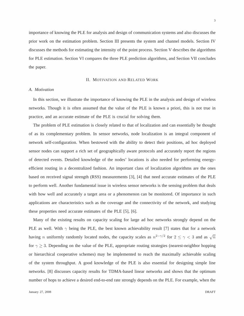
The remainder of the paper is structured as follows. SectionII provides a few examples to motivate the


3

importance of knowing the PLE for analysis and design of communication systems and also discusses the

prior work on the estimation problem. Section III presents the system and channel models. Section IV

discusses the methods for estimating the intensity of the point process. Section V describes the algorithms

for PLE estimation. Section VI compares the three PLE prediction algorithms, and Section VII concludes

the paper.

II. M OTIVATION AND RELATED WORK

A. Motivation

In this section, we illustrate the importance of knowing thePLE in the analysis and design of wireless

networks. Though it is often assumed that the value of the PLEis known a priori, this is not true in

practice, and an accurate estimate of the PLE is crucial for solving them.

The problem of PLE estimation is closely related to that of localization and can essentially be thought

of as its complementary problem. In sensor networks, node localization is an integral component of

network self-configuration. When bestowed with the abilityto detect their positions, ad hoc deployed

sensor nodes can support a rich set of geographically aware protocols and accurately report the regions

of detected events. Detailed knowledge of the nodes’ locations is also needed for performing energy-

efficient routing in a decentralized fashion. An important class of localization algorithms are the ones

based on received signal strength (RSS) measurements [3], [4] that need accurate estimates of the PLE

to perform well. Another fundamental issue in wireless sensor networks is the sensing problem that deals

with how well and accurately a target area or a phenomenon canbe monitored. Of importance in such

applications are characteristics such as the coverage and the connectivity of the network, and studying

these properties need accurate estimates of the PLE [5], [6].

Many of the existing results on capacity scaling for large adhoc networks strongly depend on the

PLE as well. Withγ being the PLE, the best known achievability result [7] states that for a network

havingn uniformly randomly located nodes, the capacity scales asn2−γ/2 for 2 ≤ γ < 3 and as√n

for γ ≥ 3. Depending on the value of the PLE, appropriate routing strategies (nearest-neighbor hopping

or hierarchical cooperative schemes) may be implemented toreach the maximally achievable scaling

of the system throughput. A good knowledge of the PLE is also essential for designing simple line

networks. [8] discusses capacity results for TDMA-based linear networks and shows that the optimum

number of hops to achieve a desired end-to-end rate stronglydepends on the PLE. For example, when the


4

desired (bandwidth-normalized) spectral efficiency exceeds the PLE, single-hop transmission outperforms

multihopping.

Energy consumption in wireless networks is a crucial issue that needs to be addressed at all the layers

of the communication system. [9] analyzes the energy consumed for several routing strategies that employ

hops of different lengths in a large network with uniformly randomly distributed nodes. Using the results

therein, we demonstrate that a good knowledge of the PLE is necessary for efficient routing. Consider

the following two simple schemes where communication is assumed to occur only in a sectorφ around

the source-destination axis.

1) Route acrossn nearest neighbor hops in a sectorφ, i.e., the next-hop node is the nearest neighbor

that lies within±φ/2 of the axis to the destination.

2) Transmit directly to then′th neighbor in the sectorφ. Here,n′ is chosen in a way that the expected

progress is the same for both schemes.

From [9], the ratio of the consumed energies for the two schemes is obtained as

E1

E2=n2Γ(1 + γ/2)Γ(n′)

Γ(n′ + γ/2),

where Γ(.) represents the Gamma function andn′ = π4 (n2 − 1) + 1. We see that the PLE plays an

important role in determining energy-efficient routing strategies. Whenγ is small, scheme 2 consumes

less energy while relaying is beneficial at high PLE values.

The performance of contention-based systems such as slotted ALOHA is very sensitive to the contention

probability p, hence it is critical to choose the optimal operating point of the system. The value of the

contention parameter is determined based on various motives such as maximizing the network throughput

[10, Eqn. 20] or optimizing the spatial density of progress [11, Eqn. 5.6]. These quantities also greatly

depend on the PLE, and therefore the optimal value of the contention probability can be chosen only

after estimatingγ.

PLE estimation is also an integral component of the cellularphone location system, which has garnered

considerable attention. There are several reasons why network providers need to estimate the position of

mobile terminals in the network. Primarily, they have to be able to assist emergency communications,

which needs accurate location estimates of the mobiles. Localization is also desired to provide positioning,

tracking and navigation services to people with special needs, such as firefighters, soldiers, elderly patients,


5

etc. Besides, knowing the PLE helps to accurately determinewhen the handoff procedure needs to be

initiated so that calls are not dropped. In addition, it helps carry out open loop power control efficiently.

B. Review of Literature

In this section, we survey some of the existing PLE estimation methods in literature. Most authors

have assumed a simplified channel model consisting only of a large-scale path loss component and a

shadowing counterpart, but we are not aware of any prior workthat has considered fading and interference

jointly in the system model. Therefore, much of the past workon PLE prediction has focused mainly on

RSS-based localization techniques. However, we remark that ignoring interference in the system model

is not realistic, in particular since PLE estimation needs to be performed even before the network is

organized.

Estimation based on a known internode distance probabilitydistribution is discussed in [12]. The

authors assume that the distance distribution between two neighboring nodesi andj is known or can be

determined easily. With the transmit power equal toP0[dBm] (assume this is a constant for all nodes),

the RSS at nodej is modeled by a log-normal behavior as

Pij [dBm] ∼ N (P ij [dBm], σ2dB),

whereσ denotes the log-normal spread andP ij [dBm] = P0[dBm]−10γ log10 dij . Now, if the neighbor’s

distance distribution is given bypR(r), then

P ij = P0ER

[

R−γ]

. (1)

E.g., if the internodal distance distribution is Rayleigh1 with mean√

π/2, then

P ij = P02−γ/2Γ(1 − γ/2). (2)

The value ofγ is obtained by equatingP ij to the empirical mean value of the received powers taken

over several node pairsi andj.

If the nearest neighbor distribution is in a complicated form that is not integrable, an idea similar to the

quantile-quantile plot can be used [12]. For cases where it might not be possible to obtain the neighbor

1The nearest neighbor distance function when the nodal arrangement is a planar Poisson point process (PPP) is Rayleighdistributed [9]. The mean value assumed is just for the sake of convenience.


6

distance distribution, the idea of estimatingγ using the concept of the Cayley-Menger determinant or

the pattern matching technique [12] is useful.

As described earlier, the situation is completely different when interference and fading are accounted

for and we cannot use the commonly known RSS-based estimators directly.

III. SYSTEM MODEL

We consider a large planar ad hoc network, where nodes are distributed as a homogeneous Poisson

point process (PPP)Φ of intensityλ (assumed unknown). Therefore, given a Borel setB, the number of

points lying in it, denoted byΦ(B), is Poisson-distributed with meanλν2(B), whereν2(·) is the two-

dimensional Lebesgue measure (area). Also, the number of points in disjoint sets are independent random

variables. The PPP model for the nodal distribution is a ubiquitously used one and may be justified by

claiming that sensor nodes are dropped from an aircraft in large numbers; for mobile ad hoc networks,

it may be argued that terminals move independently of each other.

The attenuation in the channel is modeled as a product of the large-scale path loss with exponentγ

and a flat block-fading component. To obtain a concrete set ofresults, the amplitudeH is taken to be

Nakagami-m distributed. Lettingm = 1 results in the well-known case of Rayleigh fading, while lower

and higher values ofm signify stronger and weaker fading scenarios respectively. m→ ∞ can be used

to study the case of no fading. The block fading assumption isnecessary for our analysis and may be

justified by assuming that the nodes or surrounding objects move slightly so that in each transmission

block, different fading realizations are observed. When dealing with received signal powers, we use the

power fading variable denoted byG = H2. SinceG captures the random deviation from the large-scale

path loss,EG[G] = 1. The moments ofG are [13]

EG[Gn] =Γ(m+ n)

mnΓ(m),

and the variance isσ2G(G) = 1/m.

Since the PLE estimation is usually performed during network initialization, it is fair to assume that the

transmissions in the system during this phase are uncoordinated. Therefore, we take the channel access

scheme to be ALOHA. However, for analytical tractability, we assume that transmissions occurs in time

slots. We denote the slotted ALOHA contention probability by a constantp. Consequently, the set of

transmitters forms a PPPΦ′ of intensityλp. Also, we assume that all the transmit powers are equal to


7

unity. Then, the interference at nodey on the plane is given by

IΦ(y) =∑

z∈Φ′

Gzy‖z − y‖−γ ,

wheregzy is the fading gain of the channel and‖ · ‖ denotes the Euclidean distance.

We say that communication from the transmitter atx to the receiver aty is successful if and only if

the signal-to-noise and interference ratio (SINR) aty is larger than a thresholdΘ, which depends on the

modulation and coding scheme and the receiver structure. Mathematically speaking, an outage occurs if

and only ifGxy‖x− y‖−γ

N0 + IΦ′\{x}(y)< Θ, (3)

whereIΦ\{x}(y) denotes the interference in the network aty due to all the transmitters, except the desired

one atx, andN0 is the noise power.

IV. ESTIMATION OF THE DENSITY OF THEPOISSON NETWORK

First, we furnish some basic methods to estimate the intensity of the network, which will be useful in

the later sections of the paper to estimate not only the PLE but also the parametersp andm. We also

analyze Cramer-Rao lower bounds on the MSE wherever possible.

A. The Naive Solution

The most fundamental method to estimate the network’s intensity is simply to use its definition.

Observing the process through a 2D-windowW , an unbiased estimator for the intensity is given by

λ = Φ(W )/ν2(W ). (4)

We know thatΦ(W ) is Poisson-distributed with meanλν2(W ) i.e., it is governed by a probability

mass function

f(Φ(W ) = k;λ) = exp(−λν2(W ))(λν2(W ))k

k!. (5)

The regularity condition is met in this case [14]

∂

∂λln f(Φ(W ) = k;λ) =

ν2(W )

λ

[

λ− λ]

, (6)


8

and thus, this is an efficient estimator meeting the following Cramer-Rao lower bound (CRLB) on the

error variance:

MSE(λ) = λ/ν2(W ). (7)

SinceΦ is ergodic,λ is strongly consistent in the sense that it almost surely converges to the true value

i.e., λ→ λ as the window’s area is increased. Table I consists of recorded estimates for a sample network

realization and supports the fact that the estimation errorreduces as the window size is made large. The

theoretic MSE values are also provided.

TABLE Iλ FOR VARIOUS CIRCULAR WINDOW SIZES. TRUE VALUE: λ = 1.

Window radius 25 50 75 100 200Estimate ofλ 0.9841 1.0339 1.0227 1.0190 1.0085

% Error -1.59 3.39 2.27 1.9 0.85MSE 5.1e-4 1.27e-4 5.7e-5 3.2e-5 8e-6

Onceλ has been roughly estimated, confidence intervals can be established [15]. Crow et al. provide

approximate confidence intervals forλ, employing the normal approximation and a continuity correction

[16]. If δ be the desired breadth of the confidence interval andǫ the required confidence level, then

δν2(W ) ≈[zǫ/2

2+√

1 + λν2(W )]2

−[zǫ/2

2−√

λν2(W )]2, (8)

wherezǫ/2 = Q−1(ǫ/2), and Q−1(·) is the inverse Q-function. From this, we can use the preliminary

estimate ofλ to obtain

ν2(W ) ≈4z2

ǫ/2λ

δ2. (9)

Accordingly, if one wishes to obtain an estimate of the intensity accurate to2 decimal places (δ = 0.01)

with 99% confidence (ǫ = 0.01), and a preliminary estimate ofλ = 1, ν2(W ) = 266256. A square of

side about500 units is needed to obtain an accurate estimate.

Alternatively, one can observe the process throughN disjoint windowsW1, . . . ,WN and use the

unbiased estimator

λ =1

n

N∑

i=1

Φ(Wi)

ν2(Wi). (10)

However, for nodes to be able to make these measurements, they need to have knowledge of their locations


9

and also the window boundaries. SinceΦ(Wi) are independent random variables for eachi, the following

Cramer-Rao bound is established on the MSE.

MSE(λ) ≥ λ∑N

i=1 ν2(Wi). (11)

Since this meets the regularity condition and is the minimumvariance unbiased estimator, it is also the

maximum-likelihood estimator. As a large number of windowsare considered, the MSE vanishes. Also,

if the window size is large, the MSE is nulled as seen before.

B. Estimation Based on Empty Quadrats

Here, the observation windowW is partitioned into a large number of disjoint square subregions

each of equal areaa2. The void probability for the PPP in each of those small quadrats is equal to

p0 = exp(−λa2). Equating the fraction of empty quadrats top0, λ is estimated as

λ = ln(1/p0)/a2. (12)

The estimates of the intensity for a sample realization of the PPP are shown in Table II. To obtain these

estimates, we generated a PPP with unit intensity on a150 × 150 square window and used quadrats of

sizea × a. The smallera, the more accurate is the estimate, since it is based on more quadrats, which

permits better averaging. Note that this method can also be performed with subregions of equal area that

are not necessarily squares.

TABLE IIλ USING THE EMPTY QUADRATS METHOD. TRUE VALUE OF λ = 1.

a 2 1 0.5 0.25λ 1.0366 1.0055 0.9979 0.9994

% Error 3.66 0.55 -0.21 -0.06

C. Estimation Based on Nearest Neighbor Distances

In certain situations, it might be possible to measure distances between nodes in the network. One

such case is where the location of some nodes are known and these act as beacons assisting other nodes


10

to estimate their locations. The knowledge of the nearest neighbor distances can be used to assist in

estimating the network’s intensity.

In a homogeneous Poisson network, it is well-known that the neighbor distances follow a generalized

gamma distribution [17]. Accordingly, the density of the distance to thekth-nearest neighbor for a planar

network is given by

f(dk = r;λ) = exp(−λπr2)2(λπr2)k

rΓ(k), k = 1, 2, . . . . (13)

The maximum-likelihood (ML) estimate ofλ is obtained from here by setting [14]

∂

∂λf(dk = r;λ)|λ=λML

= 0,

which gives

λML = k/πr2. (14)

For a more accurate result, we can useN beacon nodes to make aN -sized vector measurement, resulting

in the ML estimate

λML =Nk

π∑N

i=1 r2i

. (15)

10 20 30 40 50 60 70 80 90 100−0.02

0

0.02

0.04

0.06

0.08

0.1

0.12

Number of beacons N

Bia

s in

the

estim

ate

of λ

λ = 1

Nearest neighborSecond nearest neighborThird nearest neighbor

Fig. 1. The bias inλML for the kth nearest neighbor measurements captured fromN beacons fork = 1, 2, 3.


11

However, as Fig. 1 depicts, the ML estimate is biased. Moreover, the bias takes on negative values as

well. The CRLB for an unbiased estimate ofλ is given by the inverse of the Fisher information as

CRLB =1

ER

[

∂2

∂λ2 ln f(R;λ)]

=λ2

kN. (16)

10 20 30 40 50 60 70 80 90 1000

0.02

0.04

0.06

0.08

0.1

0.12

0.14

0.16

0.18

Number of beacons N

λ = 1

MSE

CRLB

k = 1

k = 2

k = 3

Fig. 2. The MSE ofλ against the CRLB for thekth nearest neighbor measurements captured fromN beacons fork = 1, 2, 3.

Fig. 2 plots the MSE and the CRLB for the estimates obtained from the first three neighbors’ distance

measurements. Though it is seen that the estimation error islowered with farther neighbors, it is harder

to make such measurements since it requires information to be relayed across more nodes.

V. PATH LOSSEXPONENT ESTIMATION

This section describes three algorithms for PLE estimationand also provides simulation results on the

estimation errors. Each method is based on a certain networkcharacteristic namely the interference

moments, the outage probabilities and the network’s connectivity properties, respectively. The PLE

estimation problem is essentially tackled by equating the practically measured values of these quantities

to the theoretically established ones to obtainγ. There is a caveat though, that needs to be addressed. In

theory, we assume that we have access to a large number of realizations and usually derive results for


12

an “average network”, that is the one obtained by averaging over all possible realizations of the nodal

distributions and channels. However, the problem in practice is that we have only a single realization of

the nodal distribution at hand. Fortunately, in the scenario where nodes are distributed as a homogeneous

PPP, we can work around this issue by using its property of ergodicity. We now state the ergodic theorem

for spatial processes that states that statistical averages of measurable functions may be replaced by spatial

averages. Using this, we argue that a single realization of the network is sufficient for accurate estimation

of the PLE.

Theorem 5.1: (Ergodic Theorem [15, p. 172]) LetT : X → X be a measure-preserving ergodic

transformation on a measure space(X,Σ, ν) and consider a “well-behaved” function2. Define the “time-

average” off , f(x) as the average over iterations ofT starting at some initial pointx. Accordingly,

f(x) = limn→∞

1

n

n−1∑

k=0

f(T kx), (17)

whereT k is thekth iterate ofT . Likewise, the spatial average off is defined as

f(x) =1

ν(X)

∫

fdν. (18)

Assuming thatν(X) is nonzero and finite,f(x) = f(x) almost everywhere.

The ergodic theorem states that for an ergodic endomorphism, the space and time averages are equal

almost everywhere. LetT denote the transformation whose iterates result in different realizations of the

PPP. Since the PPP is ergodic,T represents a measure-preserving ergodic transformation.Thus, while

f(x) reflects the average off over different realizations of the PPP at a single node,f(x) is equivalent to

taking an average over different nodes in a single realization, and these two are equal almost everywhere.

In conclusion, we remark that the estimation process can be performed in practice by looking only at a

single realization of the network and taking the necessary measurements over several nodes.

Throughout this paper, simulation results were obtained using MATLAB. The PPP was generated

by distributing a Poisson number of points uniformly randomly in a 150 × 150 square with density1.

However, in order to avoid border effects, only the nodes lying inside the inner120 × 120 square were

chosen for measurements. For analyzing the error performance of the algorithms, we used estimates

resulting from a million different realizations of the PPP.

2More precisely,f must beL1-integrable w.r.t the measureν i.e., f ∈ L1(X, Σ, ν).


13

A. Estimation Using the Moments of the Interference

A simple technique to infer the PLEγ uses the knowledge of the interference moments. Using the

estimation value of the PLE and the predicted value of the intensity of the Poisson process (from the

previous section), we can also infer the parametersp andm.

According to this method, nodes simply need to record the strength of the interference power that they

observe. By the ergodic theorem, the mean and variance of theset of measurements at several different

nodes match the theoretically determined values. We first state existing theoretic results and subsequently

describe how the estimation can be performed in practice.

For the PPP network running the slotted ALOHA protocol, thenth cumulants of the interference

resulting from transmitters in an annulus of inner radiusA and outer radiusB around the receiver node

are given as [18]

Cn = 2πλpEG[Gn]B2−nγ −A2−nγ

2 − nγ. (19)

In particular, we can consider only the caseγ > 2 (a fair assumption in a wireless scenario) and letB

to be large (considering the entire network) so that the meanand variance of the interference are

µI = C1 = 2πλpA2−γ

γ − 2(20)

and

σ2I = C2 = 2πλp

(

1 +1

m

)

A2−2γ

2γ − 2. (21)

Note that (19) states that all the moments of the interference are infinite forA = 0. However, the

large-scale path loss model is valid only in the far-field of the antenna and breaks down for very small

distances. Denote the (known) near-field radius by a positive constantA0. The algorithm based on the

interference moments works by matching the practical and theoretic values of the mean interference and

is described as follows.

• Consider an arbitrary node in the network and number it node1. Record the value of the interference

power (received power) at node 1,I1.

• Repeat the above method for several other nodes (2, . . .) recording values of interference powers

I2, . . . at the respective nodes. Eventually, the empirical mean interference(1/N)∑N

i=1 Ii averaged

overN nodes converges.


14

By the ergodic theorem, the observed mean value matches the one given by (20) withA = A0. The value

of γ can be estimated by using a look-up table and the known valuesof p and estimated intensityλ.

Alternatively, we can use a “differential method” that is based on measurements taken for two different

guard zone radii values. A guard zone is the region around a node inside which there cannot be any

transmitters. This algorithm assumes that each node has information on its location and creating guard

zones is feasible. Basically, one needs to measure the mean interference valuesµ1I andµ2

I for guard zone

radii A1 andA2 respectively. Since these observed values of the mean interference match the theoretic

values closely, we obtainµ1

I

µ2I

=

(

A1

A2

)2−γ

,

and an unbiased estimate ofγ is

γ = 2 − ln(µ1I/µ

2I)

ln(A1/A2). (22)

The advantage of the differential method is that it does not require the knowledge of the ALOHA

contention probabilityp or the intensity of the process.

Fig. 3 depicts a stem plot of the histogram of the estimated PLE values. The predicted values fit well

into a Gaussian curve (solid line) with the same statistics as the estimates, meaning that the estimation

error is approximately Gaussian in nature. The estimate ofγ is also seen to closely match its true value

of 4.

The estimateγ can be used along withλ to predict the value of the transmission probabilityp (when it

is unknown). Indeed, using (20), an estimate of the ALOHA contention parameter is obtained immediately

as

p =µ1

I(γ − 2)

2πλA2−γ1

. (23)

Furthermore, an estimate of the fading parameterm is obtained by inverting (21) as

m =

(

σ2I (γ − 1)

πλpA2−2γ1

− 1

)−1

, (24)

whereσ2I is the empirical variance of the interference for guard zoneradiusA1.

For the case that the channels are Rayleigh-faded (exponential received powers), we formulate two

other schemes for the estimation process. The first method isbased on outage probabilities, while another


15

3.8 3.85 3.9 3.95 4 4.05 4.1 4.15 4.20

0.5

1

1.5

2

2.5

3

3.5

4

4.5x 10

4 λ = 1, p = 0.75, m = 1, γ = 4, A1 = 1, A

2 = 2

Estimate of γ

Estimates of γGaussian curve

Fig. 3. Histogram ofγ for the estimation algorithm based on the interference moments. Error variance≈ 0.0015.

technique makes use of the connectivity properties of the network.

B. Estimation Based on Outage Probabilities

In the estimation procedure using the moments of the interference, a suitable guard zone needs to be

imposed around each receiver node. This might not be a practical/feasible solution, particularly in cases

where there is no relative node location information available. When it is known that the channel fading

is Rayleigh, the PLE can also be estimated using outage probabilities as discussed below. Similar to the

previous algorithm, here too, we do not need an estimate ofλ or the value ofp. We first derive some

theoretic results and then describe a practical scheme to estimateγ.

By Slivnyak’s theorem [15], the distribution of the PPP is unaffected by the addition of a point to the

process but removing it from consideration. The introduction of this point is useful in formalizing the

notion of a “typical point” of the process. Given this, consider an arbitrary node in the network and in

addition, place a transmitter at unit distance away from it3. Now, we shift the transmitter node to the

origin and consider the outage probability for this typicalnode pair. The probability of success for this

3The distance requirement is just a convenient assumption sothat when the transceivers are unit distance apart, the PLE willnot affect the received power strength


16

transceiver pair is given by

ps = E!0I [Pr(G > (N0 + I)Θ | I)]

= exp(−N0Θ)E!0I [exp (−IΘ)]

= exp(−N0Θ)MI (Θ) , (25)

whereMI(s) is the moment generating function (MGF) of the interferencepowerI andE!0I denotes the

expectation with respect to the reduced Palm measure [15]. It is basically the expectation conditioned on

there being a point at the origin0, but not including the point for calculation of the interference power.

Using the closed-form expression for the MGF [18, Eqn. 20], we have forγ > 2,

ps = c1 exp(−c2), (26)

wherec1 = exp(−N0Θ) and c2 = λpπΓ (1 + 2/γ) Γ (1 − 2/γ) Θ2/γ . The outage probability1 − ps is

plotted versusγ in Fig. 4 for different values of threshold.

2 2.5 3 3.5 4 4.5 5 5.5 60.4

0.5

0.6

0.7

0.8

0.9

1

λ = 1, p = 0.2, N0 = −80 dBm

Out

age

prob

abili

ty

γ

Θ = 20 dBΘ = 10 dBΘ = 5 dBΘ = 0 dBΘ = −5 dB

Fig. 4. Theoretical values of the outage probabilities at different thresholds.

For the rest of this subsection, we assume that the system is interference-limited. In other words,

N0 ≪ I and therefore,ps ≈ exp(−c2). We now describe a practical scheme to estimateγ. The idea


17

behind this algorithm is to compute the SIR values at each node and use the empirical distribution to

compute the success probability, which by the ergodic theorem, matches the theoretic value. It works as

follows.

• Consider an arbitrary node, call it the receiving node and place a transmitter at a unit distance away

from it. The transmitter should not belong to the original process. With a transmit power of unity,

the received power due to that transmitter alone is exponential with unit mean. Measure the SIR at

this receiver node.

• Repeat for several nodes, thus obtaining a histogram of the measured SIR values. For any given

value ofΘ, the probability of success can be empirically determined from the histogram.

The success probability obtained thus matches the one givenby (26). If it is possible to measure the value

of p, a look-up table can be generated to estimate the PLE using the known value ofp and estimated

intensity λ.

If the density of the network orp is not accurately known, we can use a differential method to estimate

γ. Accordingly, obtain histograms of the measured SINR for two different values of the threshold, say

Θ1 andΘ2. Denote the empirical values of the success probabilities corresponding to the two values of

Θ asp1s andp2

s. Theoretically, we obtain

ln(p1s)

ln(p2s)

=ln(MI(Θ1))

ln(MI(Θ2))=

(

Θ1

Θ2

)2/γ

,

and therefore an unbiased estimate ofγ is

γ =2 ln(Θ1/Θ2)

ln(ln(p1s)/ ln(p2

s)). (27)

Fig. 5 plots the histogram of the estimated PLE values when the true value isγ = 4. The estimation

error fits well into a Gaussian curve for this scheme as well.

We remark that it may not seem practical to place the transmitter for each receiver node where

measurements are taken. Instead, nodes can equivalently assume the existence of a virtual transmitter

and assume the signal power to be an exponential random variable with unit mean. This way, they can

simply measure the interference power alone and compute theSIR.

a) Error analysis when the fading distribution is not necessarily Rayleigh: A critical assumption

used for the estimation algorithm based on outage probabilities is that the fading component of the


18

3 3.5 4 4.5 5 5.50

0.5

1

1.5

2

2.5

3

3.5

4

4.5x 10

4 λ = 1, p = 0.2, γ = 4, Θ1 = 10 dB, Θ

2 = 0 dB

Estimate of γ


Fig. 5. Histogram ofγ for the method based on outage probabilities. Error variance ≈ 0.04.

channel is Rayleigh distributed. It is interesting to see how the Nakagami fading parameterm affects

the estimation results, i.e., how large the error is in the case that the fading distribution is not actually

Rayleigh, but assumed to be so. We now provide some empiricalresults to depict the behavior of the

error when the true value ofm is not unity.

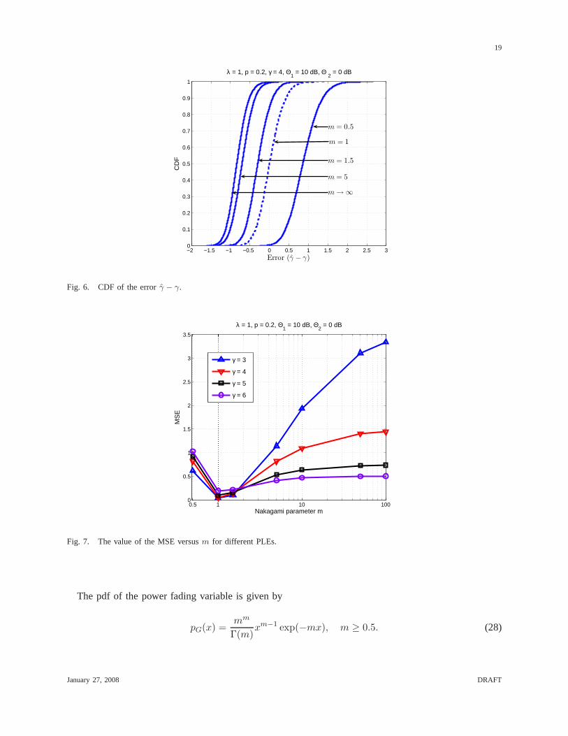
Fig. 6 shows the CDF of the error for some values ofm ranging from0.5 to ∞. For a slight deviation

of m from unity, the predicted values differ largely from the true value, particularly when the fading

effect is stronger than Rayleigh fading (0.5 ≤ m < 1). The dotted line form = 1 shows that the error

median in this case is 0. Moreover, since the error is roughlyGaussian distributed, we verify that the

estimate ofγ is indeed unbiased when the channel is Rayleigh. We also observe that the error CDF

converges asm→ ∞.

Fig. 7 plots the MSE, taken over several different network realizations versusm for different PLE

values. Again, we observe that the performance of this algorithm depends critically on the fading

parameterm especially at lower values, since a slight deviation ofm from unity largely affects the

estimation error.

As a supplement to this subsection, we now analytically derive the outage probability when the fading

componentG is a general Nakagami-m distributed variable.


19

−2 −1.5 −1 −0.5 0 0.5 1 1.5 2 2.5 30

0.1

0.2

0.3

0.4

0.5

0.6

0.7

0.8

0.9

1

Error (γ − γ)

CD

F

λ = 1, p = 0.2, γ = 4, Θ1 = 10 dB, Θ

2 = 0 dB

m = 0.5

m = 1

m = 1.5

m = 5

m→ ∞

Fig. 6. CDF of the errorγ − γ.

0.5 1 10 1000

0.5

1

1.5

2

2.5

3

3.5

Nakagami parameter m

MS

E

λ = 1, p = 0.2, Θ1 = 10 dB, Θ

2 = 0 dB

γ = 3

γ = 4

γ = 5

γ = 6

Fig. 7. The value of the MSE versusm for different PLEs.

The pdf of the power fading variable is given by

pG(x) =mm

Γ(m)xm−1 exp(−mx), m ≥ 0.5. (28)


20

Using this, we have

ps = E!0I [Pr(G > IΘ | I)]

= E!0I

[∫ ∞

IΘ

mm

Γ(m)xm−1 exp(−mx)dx

]

=1

Γ(m)

∫ ∞

0Γ(m,xΘm)PI(x)dx, (29)

whereΓ(·, ·) is the upper incomplete gamma function4 andPI(x) denotes the pdf of the interference

function.

The expressions can be further simplified whenm is an integer. Form ∈ Z+, we have

ps(a)=

m−1∑

k=0

1

k!

∫ ∞

0(xΘm)k exp(−xΘm)PI(x)dx

(b)=

m−1∑

k=0

(−Θm)k

k!

dk

dskMI(s)|s=Θm, (30)

where(a) is obtained from the series expansion of the upper incomplete gamma function and(b) from

the definition of the MGF. We also have the following closed-form expression for the MGF [18, Eqn.

20]

MI(s) = exp(−λpπEG[G2/γ ]Γ(1 − 2/γ)s2/γ).

Using this, we get

ps = exp(−c3)m−1∑

k=0

ck3k!

(

2

γ

)k

, (31)

wherec3 = λpπEG(G2/γ)Γ(1−2/γ)(Θm)2/γ . The outage probabilities at integer values ofm for γ > 2

can be numerically evaluated from the above equation.

C. Estimation Based on the Cardinality of the Transmitting Set

In this subsection, we present a method to estimate the PLE based on the connectivity properties of the

network. For any node, define its transmitting set as the group of transmitting nodes whom it receives a

packet from, in a given time slot. More formally, for receiver y, transmitter nodex is in its transmitting

set if they are connected i.e., the SINR aty is greater than a certain thresholdΘ. Note that this set

4Mathematica: Gamma[a,z]


21

changes from time slot to time slot. This algorithm is based on matching the theoretic and practical

values of the mean number of elements in the transmitting set. Note that forΘ = 0 dB, the condition

for a transceiver pair to be connected is that the received signal strength is greater than the interference

power. Thus, forΘ ≥ 1, the cardinality of the transmitting set can at most be one, and that transmitter is

the one with the best channel to the receiver. The following proposition forms the basis of the estimation

algorithm.

Proposition 5.2: Under the conditions of Rayleigh fading andN0 ≪ I, the cardinality of the transmit-

ting set is well-approximated by a Poisson distribution with parameter(Γ(1 + 2/γ)Γ(1 − 2/γ)Θ2/γ)−1.

Proof: Extending the procedure used for deriving (26), we see that the success probability for a

transceiver pair at an arbitrary distanceR units apart is

ps(R) = c′1(R) exp(−c2R2),

wherec′1(R) = exp(−N0RγΘ). ForN0 ≪ I, ps ≈ exp(−c2R2). Now, we place an additional receiver

node O at the origin (which does not affect the distribution of the PPP) and analyze the transmitting set

for this “typical” node.

Consider a disc of radiusa centered at the origin. LetEi denote the event that theith transmitter

inside this disc is in O’s transmitting set. ForR uniformly distributed in[0, a], we have

P(Ei) = ER[ps(R) | R]

=2π

πa2

∫ a

0re−c2r2

dr

=1

a2c2(1 − e−a2c2). (32)

Note that in any given time slot, the eventsEi andEj for arbitrary transmittersi and j are actually

slightly correlated. This is becausei acts as an interferer forj’s signal and vice versa. We neglect this

minor dependence and assume that theEi’s are independent events. Also, sinceP(Ei) is independent of

i, we takeP(Ei) = P(E), ∀i, to simplify notation. Denote the mean number of transmitters in the disc

of radiusa by Na = λpπa2. Then, the probability of having exactlyk elements in the transmitting set


22

T is calculated as

P(NT = k) = lima→∞

EN :N≥k

[(

N

k

)

P(E)k(1 − P(E))N−k

]

= lima→∞

∞∑

n=k

e−NaNna

n!

(

n

k

)

P(E)k(1 − P(E))n−k

(a)= lim

a→∞

(P(E)Na)k

k!

∞∑

s=0

e−NaN sa

s!· (1 − P(E))s

= lima→∞

(P(E)Na)k

k!exp(−NaP(E))

= exp(−c4)ck4/k!, (33)

where (a) is obtained on using the substitutionn − k = s, and c4 = lima→∞NaP(E) = 1/(Γ(1 +

2/γ)Γ(1 − 2/γ)Θ2/γ).

Therefore, the cardinality of the transmitting set,NT , is distributed as a Poisson random variable

with meanc4, and is, surprisingly, independent ofλ and p. Because of the homogeneity in the nodal

arrangement, the size of each node’s transmitting set obeysthe same statistics. Fig. 8 plots the theoretic

expected size of the transmitting setNT for different threshold values at various PLE values.

2 2.5 3 3.5 4 4.5 5 5.5 60

0.2

0.4

0.6

0.8

1

1.2

1.4

Ave

rage

car

dina

lity

of th

e tr

ansm

ittin

g se

t

Path loss exponent γ

Θ = −5 dB

Θ = 0 dB

Θ = 5 dB

Θ = 10 dB

Θ = 20 dB

Fig. 8. The mean number of elements in the transmitting set versusγ for different SIR threshold values.


23

Comparing the empirical mean cardinality of the transmitting set toc4, γ can be estimated using a

look-up table. Alternatively, we may use a differential method where we measure the mean cardinalities

of the transmitting sets for two different values ofΘ, Θ1 andΘ2. Denote the mean transmitting set sizes

corresponding to the two values ofΘ as N1T andN2

T . Theoretically, we obtain

N1T

N2T

=

(

Θ2

Θ1

)2/γ

,

giving us an unbiased estimate as

γ =2 ln(Θ2/Θ1)

ln(N1T /N

2T ). (34)

3 3.2 3.4 3.6 3.8 4 4.2 4.4 4.6 4.8 50

0.5

1

1.5

2

2.5

3

3.5

4x 10

4 λ = 1, p = 0.2, γ = 4, Θ1 = 10 dB, Θ

2 = 0 dB

Estimate of γ


Fig. 9. Histogram ofγ for the estimation algorithm based on the cardinality of thetransmitting set. Error variance≈ 0.03.

Fig. 9 plots the histogram of the estimated PLE values when the actual value isγ = 4. The estimation

error for this scheme also seems approximately Gaussian.

We now analytically evaluate the Cramer-Rao lower bound for an unbiased estimate ofNT . From (33),

we have

ln f(NT = k; γ) = −c4 + k ln(c4) − ln(k!) (35)


24

The Fisher information for an unbiased estimate ofγ is then given by

J(γ) = ENT

[

− ∂2

∂γ2ln f(NT ; γ)

]

=1

c4

(

∂c4∂γ

)2

=4[

ψ(1 − 2γ ) − ψ(1 + 2

γ ) − ln(Θ)]2

γ4Γ(1 + 2γ )Γ(1 − 2

γ )Θ2

γ

, (36)

whereψ(x) represents the digamma function5 and has the integral representation

ψ(x) =

∫ ∞

0

(

e−t

t− e−xt

1 − e−t

)

dt.

We have CRLB= 1/J(γ).

b) Error Analysis when the fading distribution is not necessarily Rayleigh: The method based on

the cardinality of the transmitting set assumes that channel is Rayleigh-faded. It is interesting to see how

large the error is when the true value ofm is not 1. We now derive some analytical results showing the

dependence of the algorithm on the fading parameterm. Specifically, we determine the distribution of

NT for integer values ofm and comment on its effect on the estimation algorithm.

WhenG is a Nakagami-m distributed variable, we can generalize (31) to obtain the success probability

for a transceiver pair at an arbitrary distanceR units apart as

ps(R) =m−1∑

k=0

exp(−c3R2)(

c3R2)k

k!

(

2

γ

)k

, m ∈ Z+. (37)

5Mathematica: PolyGamma[x]


25

Using this, we obtain

P(E) = ER[ps(R) | R]

=2π

πa2

∫ a

0

m−1∑

k=0

exp(−c3r2)r2k

k!

(

2c3γ

)k

rdr

=1

a2

m−1∑

k=0

(

2c3γ

)k ∫ a

0

exp(−c3r2)k!

r2k2rdr

(a)=

1

a2c3

m−1∑

k=0

(

2

γ

)k 1

k!

∫ c3a2

0tk exp(−t)dt

(b)=

1

a2c3

m−1∑

k=0

(

2

γ

)k 1

k!

(

1 − Γ(k + 1, c3a2))

, (38)

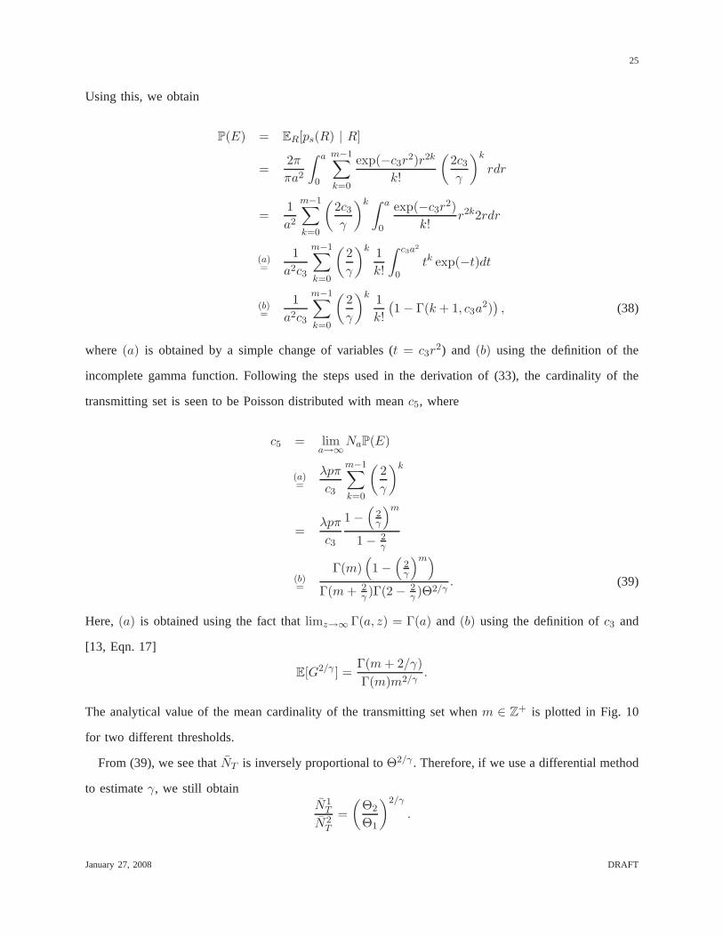
where (a) is obtained by a simple change of variables (t = c3r2) and (b) using the definition of the

incomplete gamma function. Following the steps used in the derivation of (33), the cardinality of the

transmitting set is seen to be Poisson distributed with meanc5, where

c5 = lima→∞

NaP(E)

(a)=

λpπ

c3

m−1∑

k=0

(

2

γ

)k

=λpπ

c3

1 −(

2γ

)m

1 − 2γ

(b)=

Γ(m)(

1 −(

2γ

)m)

Γ(m+ 2γ )Γ(2 − 2

γ )Θ2/γ. (39)

Here,(a) is obtained using the fact thatlimz→∞ Γ(a, z) = Γ(a) and (b) using the definition ofc3 and

[13, Eqn. 17]

E[G2/γ ] =Γ(m+ 2/γ)

Γ(m)m2/γ.

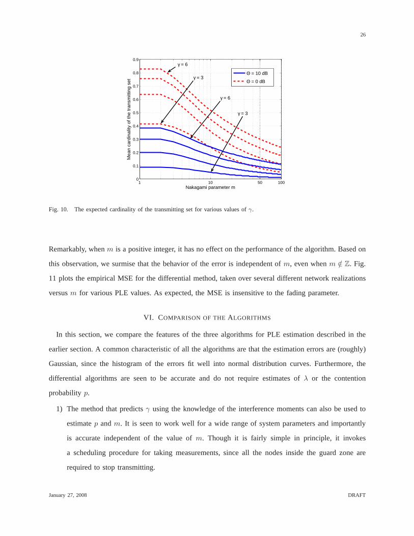
The analytical value of the mean cardinality of the transmitting set whenm ∈ Z+ is plotted in Fig. 10

for two different thresholds.

From (39), we see thatNT is inversely proportional toΘ2/γ . Therefore, if we use a differential method

to estimateγ, we still obtainN1

T

N2T

=

(

Θ2

Θ1

)2/γ

.


26

1 10 50 1000

0.1

0.2

0.3

0.4

0.5

0.6

0.7

0.8

0.9


Mea

n ca

rdin

ality

of t

he tr

ansm

ittin

g se

t

Θ = 10 dB

Θ = 0 dBγ = 3

γ = 6

γ = 6

γ = 3

Fig. 10. The expected cardinality of the transmitting set for various values ofγ.

Remarkably, whenm is a positive integer, it has no effect on the performance of the algorithm. Based on

this observation, we surmise that the behavior of the error is independent ofm, even whenm /∈ Z. Fig.

11 plots the empirical MSE for the differential method, taken over several different network realizations

versusm for various PLE values. As expected, the MSE is insensitive to the fading parameter.

VI. COMPARISON OF THEALGORITHMS

In this section, we compare the features of the three algorithms for PLE estimation described in the

earlier section. A common characteristic of all the algorithms are that the estimation errors are (roughly)

Gaussian, since the histogram of the errors fit well into normal distribution curves. Furthermore, the

differential algorithms are seen to be accurate and do not require estimates ofλ or the contention

probability p.

1) The method that predictsγ using the knowledge of the interference moments can also be used to

estimatep andm. It is seen to work well for a wide range of system parameters and importantly

is accurate independent of the value ofm. Though it is fairly simple in principle, it invokes

a scheduling procedure for taking measurements, since all the nodes inside the guard zone are

required to stop transmitting.


27

1 10 1000.50.015

0.02

0.025

0.03

0.035

0.04

0.045

0.05

0.055

0.06


MS

E

λ = 1, p = 0.2, Θ1 = 10 dB, Θ

2 = 0 dB

γ = 3

γ = 4

γ = 5

γ = 6

Fig. 11. The value of the MSE versusm for different PLEs.

2) The scheme that estimatesγ upon calculating outage probabilities does not need a guardzone to

be imposed, but requires a transmitter that originally did not belong to the process to be placed

at unit distance from the receiver. Moreover, it is formalized only for the Rayleigh fading case

(m = 1). The error is seen to be high when fading is severe (values ofm lower than1), and

more so when the PLE is high. Also, this algorithm is convenient to use only when the network is

interference-limited, i.e., the noise level is considerably lower than the interference power.

3) The algorithm based on the connectivity properties of thePPP does not need any node location

information or the imposition of a guard zone around the nodes. Furthermore, it is robust in the

sense that it performs independently of the value of the fading parameterm. Like the previous

algorithm, it is, however, based on the condition that the system is interference-limited.

We now address a couple of performance issues related to the rate of convergence of the algorithms.

First, the success of these methods is critically determined by the number of survey pointsN to be taken.

A small value ofN will result in low accuracy while a large value ofN will result in an expensive survey

process with many of the survey points giving little benefit.The second aspect is related to centralized

versus distributed information processing. Specifically,the efficiency of these techniques relies on how

the nodes that take measurements are chosen. Consider the two extreme cases where nodes1, 2, . . . N


28

can be chosen in a random fashion or as subsequent nearest neighbors. In the latter method, the first

node relays its measurement information to its nearest neighbor which then passes this on along with its

own measured value, to its nearest neighbor other than the first node, and information is propagated in

this manner. If nodes are chosen this way in a local fashion, the measurements will be correlated and

the algorithm takes a long time to converge. On the other hand, choosing nodes randomly may result in

choosing nodes sufficiently far apart but will also incur a lot of overhead when information needs to be

exchanged between nodes or relayed to a central server or a fusion center.

Fig. 12 compares the performance of the three algorithms. Here, R refers to the centralized computing

scheme where measurements are taken at randomly picked nodes and relayed to the central server,

while NN refers to the distributed algorithm where measurements are passed over to subsequent nearest

neighbors. From the plot, we see that the algorithm based on the interference moments clearly has the

lowest MSE. Also, for the first two schemes, choosing randomly located nodes for measurements leads to

a much faster convergence than when choosing subsequent nearest neighbors. However, for the method

based on the cardinality of the transmitting set, the order in which nodes are picked does not have a

huge impact on its convergence rate.

100 200 300 400 500 600 700 800 900 100010

−3

10−2

10−1

100

101

Number of measurements taken

MS

E

λ = 1, γ = 4, m = 1

Algo 1 − RAlgo 2 − RAlgo 3 − RAlgo 1 − NNAlgo 2 − NNAlgo 3 − NN

Fig. 12. Comparison of the MSE performance of the three algorithms.


29

Our algorithms work well even with more general point process models. We tested them for networks

with two other forms of nodal distribution, the Matern hard core process and the Thomas clustered

process [15], and the estimated PLE values are seen to accurately match the true values.

Finally, we remark that in reality, the PLE value changes depending on the terrain category and the

environmental conditions, and hence cannot always be assumed to be a constant over the entire network.

However, our algorithms are still useful since they can be used for obtaining local estimates, based on

measurements taken over neighborhoods. For cases where thechannel behavior is different for different

regions of the network, it can be divided into sub-areas withconstantγ that are analyzed separately.

VII. C ONCLUSION

In wireless systems, the value of the PLE is critical but not known a priori, thus an accurate estimate is

essential for the analysis and design of systems. We offer a novel look at the issue of PLE estimation in a

large wireless network, by taking into account Nakagami-m fading, the underlying node distribution and

the network interference. Nodes are assumed to be arranged as a homogeneous PPP on the plane and the

channel access scheme is slotted ALOHA. For such a system, the paper describes three separate algorithms

for PLE estimation. Simulation results are provided to demonstrate their performance and quantify the

estimation errors. For each of the algorithms, we find that the estimation error is approximately Gaussian.

Comparing the algorithms, we see that the one that is based onthe interference moments performs the

best in terms of minimizing the MSE. We also provide methods to infer the intensity of the PPP and

evaluate Cramer-Rao lower bounds on the MSE.

REFERENCES

[1] T. S. Rappaport,Wireless Communications - Principles and Practice, Prentice Hall, 1991.

[2] W. C. Jakes, “Microwave Mobile Communications,” Wiley-IEEE Press, May 1994.

[3] A. Savvides, W. L. Garber, R. L. Moses and M. B. Srivastava, “An Analysis of Error Inducing Parameters in Multihop

Sensor Node Localization,”IEEE Transactions on Mobile Computing, Vol. 4, No. 6, pp. 567-577, Nov./Dec. 2005.

[4] N. Patwari, I. Hero, A. O. M. Perkins, N. Correal, and R. ODea, “Relative Location Estimation in Wireless Sensor

Networks,” IEEE Transactions on Signal Processing, Vol. 51, No. 8, pp. 2137-2148, Aug. 2003.

[5] C. Bettstetter, “On the Connectivity of Ad Hoc Networks,” The Computer Journal, Special Issue on Mobile and Pervasive

Computing, Vol. 47, No. 4, pp. 432-447, July 2004.

[6] D. Miorandi and E. Altman, “Coverage and Connectivity ofAd Hoc Networks in the Presence of Channel Randomness,”

IEEE INFOCOM, Mar. 2005.


30

[7] A. Ozgur, O. Leveque and D. Tse, “Hierarchical Cooperation Achieves Optimal Capacity Scaling in Ad Hoc Networks,”

IEEE Transactions on Information Theory, Vol. 53, No. 10, pp. 3549-3572, Oct. 2007.

[8] M. Sikora, J. N. Laneman, M. Haenggi, D. J. Costello, Jr.,and T. E. Fuja, “Bandwidth- and Power-Efficient Routing in

Linear Wireless Networks,”IEEE Transactions on Information Theory, Vol. 52, No. 6, pp. 2624-2633, June 2006.

[9] M. Haenggi, “On Routing in Random Rayleigh Fading Networks,” IEEE Transactions on Wireless Communications, Vol.

4, No. 4, pp. 1553-1562, July 2005.

[10] J. Venkataraman, M. Haenggi and O. Collins, ”Shot NoiseModels for Outage and Throughput Analyses in Wireless Ad

Hoc Networks,”Military Communications Conference (MILCOM’06), Washington DC, Oct. 2006.

[11] F. Baccelli, B. Błaszczyszyn and P. Muhlethaler, “An Aloha Protocol for Multihop Mobile Wireless Networks,” IEEE

Transactions on Information Theory, Vol. 52, No. 2, pp. 421-436, Feb. 2006.

[12] G. Mao, B. D. O. Anderson and B. Fidan, “Path Loss Exponent Estimation for Wireless Sensor Network Localization,”

Computer Networks, Vol. 51, Iss. 10, pp. 2467-2483, July 2007.

[13] M. Nakagami,The m-distribution : A General Formula for Intensity Distribution of Rapid Fading, in W. G. Hoffman,

“Statistical Methods in Radiowave Propagation,” PergamonPress, Oxford, U. K., 1960.

[14] S. M. Kay, “Fundamentals of Statistical Signal Processing, Volume I: Estimation Theory,” Prentice Hall, Mar. 1993.

[15] D. Stoyan, W. S. Kendall and J. Mecke, “Stochastic geometry and its applications,” Wiley & Sons, 1978.

[16] Edwin L. Crow; Robert S. Gardner, “Confidence Intervalsfor the Expectation of a Poisson Variable,”Biometrika, Vol.

46, No. 3/4, pp. 441-453, Dec. 1959.

[17] M. Haenggi, “On Distances in Uniformly Random Networks,” IEEE Transactions on Information Theory, vol. 51, pp.

3584-3586, Oct. 2005.

[18] S. Srinivasa and M. Haenggi, “Modeling Interference inFinite Uniformly Random Networks,”International Workshop

on Information Theory for Sensor Networks (WITS ’07), Santa Fe, June 2007.


1 Path Loss Exponent Estimation in Large Wireless …mhaenggi/pubs/tsp08.pdf1 Path Loss Exponent...

Documents

Transcript of 1 Path Loss Exponent Estimation in Large Wireless …mhaenggi/pubs/tsp08.pdf1 Path Loss Exponent...