1

On the Computation of the Permanent

Dana Moshkovitz

2

Overview

Presenting the problem Introducing the Markov chain Monte-Carlo

method.

3

Perfect Matchings in Bipartite Graphs

An undirected graph G=(UV,E) is bipartite if

UV= and EUV.

A 1-1 and onto function f:UV is a perfect

matching if for any uU, (u,f(u))E.

4

Finding Perfect Matchings is Easy

Matching as a flow problem

5

What About Counting Them? Let A=(a(i,j))1i,jn be the adjacency

matrix of a bipartite graph G=({u1,...,un}{v1,...,vn},E), i.e. -

n

i

iiaAper1

))(,()(

otherwise

Evujia ji

0

),(1),(

permanent sum over the permutations of {1,...,n}

The number of perfect matchings in the graph is

1010

0101

1011

0011

6

Cycle-Covers

• Given an undirected bipartite graph G=({u1,...,un}{v1,...,vn},E), the corresponding directed graph is G’=({w1,...,wn},E), where (wi,wj)E iff (ui,vj)E.

• Definition: Given a directed graph G=(V,E), a set of node-disjoint cycles that together cover V is called a cycle-cover of G.

• Observation: Every perfect matching in G corresponds to a cycle-cover in G’ and vice-versa.

7

Three Ways To View Our Problem

1) Counting the number of Perfect Matchings in a bipartite graph.

2) Computing the Permanent of a 0-1 matrix.

3) Counting the number of Cycle-Covers in a directed graph.

8

#P - A Complexity Class of Counting Problems• LNP iff there is a polynomial time decidable

binary relation R, s.t.

),(|)(| yxRxp|y|yLx

• f #P iff f(x)=| { y | R(x,y) } | where R is a relation associated with some NP problem.• We say a #P function is #P-Complete, if every #P function Cook-reduces to it.• It is well known that #SAT (i.e - counting the number of satisfying assignments) is #P-Complete.

some polynomial

9

On the Hardness of Computing the Permanent

Claim [Val79]: Counting the number of cycle-covers in a directed graph is #P-Complete.

Proof: By a reduction from #SAT to a generalization of the problem.

10

The Generalization: Integer Permanent

2

3

12

020

100

032

Activity: an integer weight attached to each edge (u,v)E, denoted (u,v).

The activity of a matching M is (M)=(u,v)M(u,v).

The activity of a set of matchings S is (M)=MS(M).

The goal is to compute the total activity.

2

2

3

1

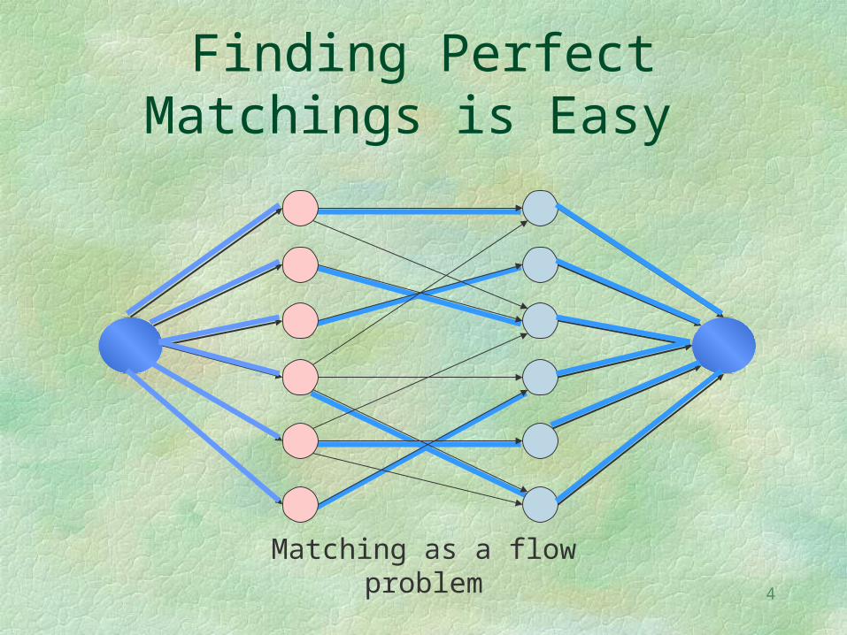
11

Integer Permanent Reduces to 0-1 Permanent

2

the rest of the graph

1

1

We would have loved to do something of this sort...

12

Integer Permanent Reduces to 0-1 Permanent

the rest of the graphSo instead we do:

13

But this is really cheating!The integers may be exponentially large, but we are forbidden to add an exponential number of nodes!

14

The Solution

the rest of the graph

...

15

What About Negative Numbers?

Without loss of generality, let us assume the only negative numbers are -1’s.

We can reduce the problem to calculating the Permanent modulo (big enough) N of a 0-1 matrix by replacing each -1 with (N-1).

Obviously, Perm mod N is efficiently reducible to calculating the Permanent.

16

Continuing With The Hardness Proof

We showed that computing the permanent of an integer matrix reduces to computing the permanent of a 0-1 matrix.

It remains to prove the reduction from #SAT to integer Permanent.

We start by presenting a few gadgets.

17

The Choice Gadget

Observation: in any cycle-cover the two nodes must be covered by either the left cycle (true) or the right cycle (false).

x= true x= false

18

The Clause Gadget

Observation: no cycle-cover of this

graph contains all three external edges.

However, for every proper subset of the external edges, there is exactly one cycle-cover containing it.

each external edge corresponds to one

literal

19

The Exclusive-Or Gadget

The Perm. of the whole matrix is 0.

The Perm. of the matrix resulting if we delete the first (last) row and column is 0.

The Perm. of the matrix resulting if we delete the first (last) row and the last (first) column is 4.

-1

-1

23

-1

0310

2110

1111

1110

20

Plugging in the XOR-GadgetObserve a cycle-cover of the graph with a XOR-

gadget plugged as in the below figure. If e is traversed but not t (or vice versa), the

Perm. is multiplied by 4. Otherwise, the Perm. is added 0.

e

t

21

Putting It All Together

One choice gadget for every variable.

One Clause gadget for every clause.

x= true x= falseif the literal is x

x= true x= false

if the literal is x

22

Sum Up

Though finding a perfect matching in a bipartite graph can be done in polynomial time,

counting the number of perfect matchings is #P-Complete, and hence believed to be impossible in polynomial time.

So what can we do?

23

Our Goal - FPRAS for Perm

Describing an algorithm, which given a 0-1 nn matrix M and an >0, computes, in time polynomial in n and in -1, a r.v Y, s.t

Pr[(1-)Perm(M) Y (1+)Perm(M)] 1-, where 0< ¼.

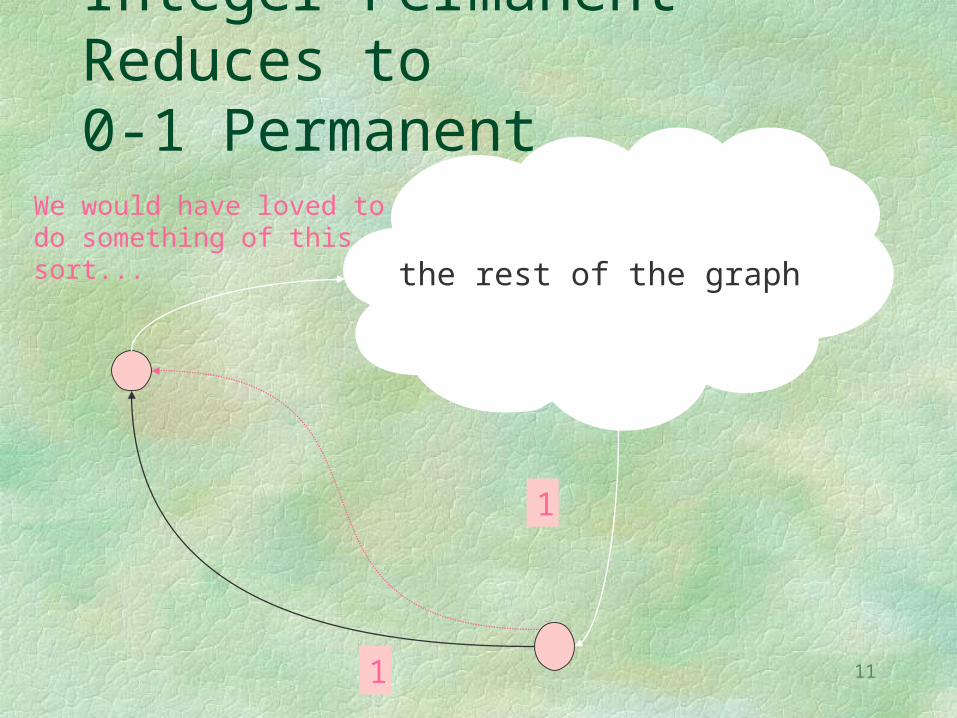
24

The Markov Chain Monte Carlo Method

Let be a very large (but finite) set of combinatorial structures,

and let be a probability distribution on . The task is to sample an element of

according to the distribution .

The Connection to Approximate Counting

U

G

The Monte-Carlo method: Choose at random u1,...,uNU.

Let Y=|{i : uiG }|.

Output Y|U|/N.

||4

|| 2

21||)1(||

||)1(Pr U

GN

eGN

UYG

Analysis: By standard Chernoff bound,

||

||12ln4

2 G

UN

26

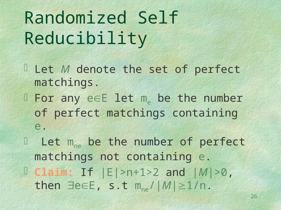
Randomized Self Reducibility

Let M denote the set of perfect matchings.For any eE let me be the number of perfect

matchings containing e. Let mne be the number of perfect matchings not

containing e.Claim: If |E|>n+1>2 and |M|>0, then eE, s.t

mne/|M|1/n.

27

Counting Reduces to Sampling

PermFPRAS(G)Input: a bipartite graph G=(VU,E).Output: an approximation for |M|.1. if |E|n+1 or n<2, compute |M| exactly.2. for each eE do 3. sample 4n|E|2ln(2|E|/)/2 perfect matchings 4. Y fraction of matchings not containing e.5. if Y1/n, return PermFPRAS(VU,E\{e})/Y

28

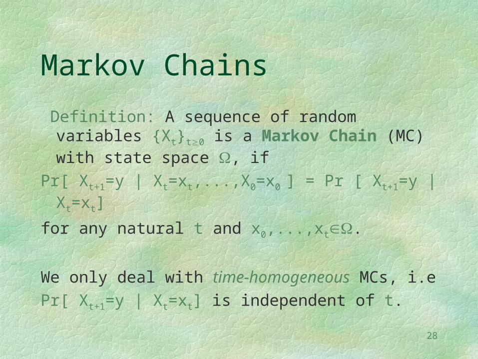
Markov Chains

Definition: A sequence of random variables {Xt}t0 is a Markov Chain (MC) with state space , if

Pr[ Xt+1=y | Xt=xt,...,X0=x0 ] = Pr [ Xt+1=y | Xt=xt]

for any natural t and x0,...,xt.

We only deal with time-homogeneous MCs, i.e

Pr[ Xt+1=y | Xt=xt] is independent of t.

29

Graph Representation of MC

Conceptually, A Markov chain is a HUGE directed weighted graph.

The nodes correspond to the objects in .

Xt = position in step t.

The weight of (x,y) is P(x,y)=Pr[X1=y|X0=x].

0.5

0.15

0.5

0.05

0.5

0.1

0.1

0.60.1

0.2

0.05

0.20.1

0.85

0.15

0.55

0.1

0.8

30

Iterated Transition

Definition: For any natural t,

i.e - Pt(x,y)=Pr[Xt=y|X0=x].

0),'()',(

0),(),(

'

1 tyyPyxP

tyxIyxP

y

tt

31

More Definitions

A MC is irreducible, if for every pair of states x,y, there exists tN, s.t.

Pt(x,y)>0. A MC is aperiodic, if

gcd{t : Pt(x,x) > 0}=1

for any x.A finite MC is ergodic if it is

both irreducible and aperiodic.

0.5

0.3

0.5

0.2

0.5

0.1

0.1

0.9

32

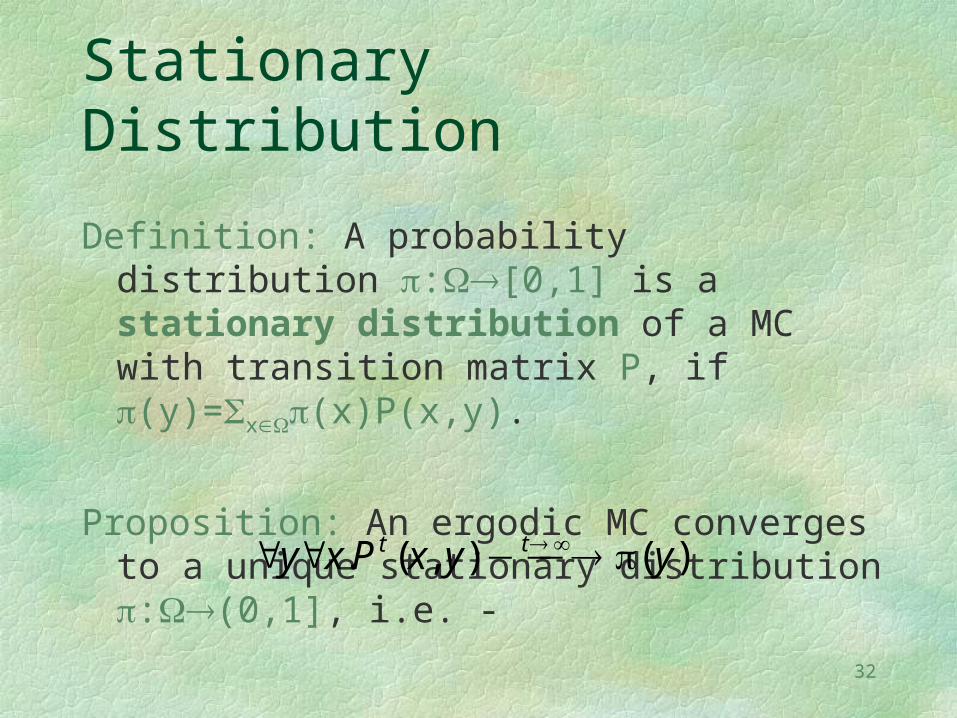
Stationary Distribution

Definition: A probability distribution :[0,1] is a stationary distribution of a MC with transition matrix P, if (y)=x(x)P(x,y).

Proposition: An ergodic MC converges to a unique stationary distribution :(0,1], i.e. -

)(),(. yyxPxy tt

33

Time Reversible Chains

Definition: Markov chains for which some distribution satisfies for all M,M’,

(the detailed balance condition)

are called (time) reversible. Moreover, that is the stationary distribution.

)',(:),'()'()',()( MMQMMPMMMPM

34

Mixing Time

Definition: Given a MC with transitions matrix P and stationary distribution , we define the mixing time as

x()=min{ t : ½y |Pt(x,y)-(y)| }

Definition: A MC is rapidly mixing, if for any fixed >0. x() is bounded above by a polynomial.

35

Conductance

Definition: the conductance of a reversible MC is defined as =minS(S), where

Theorem: For an ergodic, reversible Markov chain with self loops probabilities P(y,y)½ for all states x,

)()(

),(

)()(

),()(

SS

yxQ

SS

SSQS Sx Sy

)ln)((ln2

)( 112

xx

36

Framework

MC: ,

irreducibleaperiodic

ergodic

½ self loops

detailed balance condition

stationary

reversible

rapid mixing

1/poly

37

Our Markov Chain

The state space will consist of all perfect and near-perfect (size n-1) matchings in the graph.

The stationary distribution will be uniform over the perfect matchings and will assign them probability O(1/n2).