
1 Notes of Econ424 Part 1: Excel Spring 2008 Ginger Z. Jin ginger
83
1 Notes of Econ424 Part 1: Excel Spring 2008 Ginger Z. Jin http:// www.glue.umd.edu /~ginger/
-
Upload
ashley-cecily-rogers -
Category
Documents
-
view
221 -
download
0
Transcript of 1 Notes of Econ424 Part 1: Excel Spring 2008 Ginger Z. Jin ginger
1
Notes of Econ424Part 1: Excel
Spring 2008
Ginger Z. Jin
http://www.glue.umd.edu/~ginger/
2
Class 1: Introduction
• Goal of this class
• Syllabus
• First-class questionnaire
• Logins
• A peek at the data collected by the questionnaire
3
"There are three kinds of lies – lies, damned lies and statistics."
--- (?) Mark TwainWinston ChurchillBenjamin Disraeli

4
Statistical manipulation
– Randomness behind each statistics• News tend to report outliers or new observation that deviates
from the status quo• Newsworthy is not equal to good statistics
– Correlation and causation• Harvard graduates earn more than high school dropouts, this
does not mean these dropouts, if given a Harvard diploma, will earn as much
– Report favorable information while hide measurement error / variable definition
5
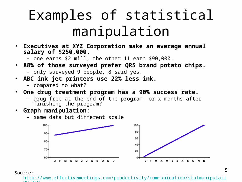
Examples of statistical manipulation
• Executives at XYZ Corporation make an average annual salary of $250,000.
– one earns $2 mill, the other 11 earn $90,000. • 88% of those surveyed prefer QRS brand potato chips.
– only surveyed 9 people, 8 said yes. • ABC ink jet printers use 22% less ink.
– compared to what?• One drug treatment program has a 90% success rate.
– Drug free at the end of the program, or x months after finishing the program?• Graph manipulation:
– same data but different scale
Source: http://www.effectivemeetings.com/productivity/communication/statmanipulation.asp

6
Real examples• Kerry: Now, the president has presided over an economy where we've
lost 1.6 million jobs. – there are by 1.6 million private sector job loss since Bush took office, but the drop
in total payroll employment -- including teachers, firemen, policemen and other federal, state and local government employees is down by 821,000.
Source: http://www.factcheck.org/article275.html
• An internet ad by the Democratic Senatorial Campaign Committee: there were "four times as many terror attacks in 2005“ (as compared to 2004).
– National Counter Terrorism Center: The previously used statutory definition of "international terrorism" ("involving citizens or territory of more than one country") resulted in hundreds of incidents per year; the currently used statutory definition of "terrorism" ("premeditated, politically motivated violence perpetrated against noncombatant targets") results in many thousands of incidents per year.
Source: http://www.factcheck.org/article417.html

7
My goal
At the end of the semester:
• You feel comfortable collecting, locating and analyzing real data
• You are able to read, interpret and criticize statistics generated by other people
• Given a real data set, you are able to generate basic statistics by yourself and give them meaningful interpretations

8
Syllabus is at:
http://www.glue.umd.edu/~ginger/Click on “ECON424” at the bottom
Assign project 1

9
Class 2: Introduction to Excel
Handout from UMD peer training• Open a file in N:\ and save it (as .xls or .csv) in
M:\.• Define observation and variable• Hide/unhide rows/columns, freeze panes• Change excel settings (Tools+options)• Change cell/column/row formats• Highlight (shift+, ctrl+) • Formulas/dragdowns• Charts
10
Class 2: More on Excel
Three more items on excel:
• Text to columns
• Insert text box in excel
• Transport excel table and chart into MS words

11
Class 3: Data Collection (e.stat chapter 3)
• Start with a question– characterize facebook usage among 18-25
• Define observation– an individual, a class, a school?
• Define variables– use or not, intensity of usage, scope of usage
• Define sample– Students enrolled? Students attending the
first class? Students attending the first class and use facebook?

12
Data Collection (continued)
• Methods of data collection– Field collection by hand– Experiment– Survey / Questionnaire
• In class• By phone • By email• Follow up survey
– Existing data sources (library, internet, etc.)

13
Data Collection (continued)
• Things that need special attention– Measurement error
• data collector’s preference, if revealed in the survey, may bias respondent answer
• self report may be biased in a specific direction• anonymous vs. identity-revealing
– Sample selection • sample not representative by design (those attending first
class are different from those who don’t attend)• missing values generate sample selection (need a follow
up?)– Sample size and balance
• variations in the studied variables• trade off between statistical power and cost of data collection• similar size of comparable subsamples
14
Role playing• To better understand subprime mortgage financial
crisis, what statistics would you generate and analyze if you are the head of:
– Federal Reserve – Wall Street Journal– New York Stock Exchange– Countrywide Financial– National Association of Realtors– European Central Bank

15
Background of subprime mortgage financial crisisfinal borrower with poor credit
Bank / Mortgage companies
subprime loans (low introductory rates, insufficient income check, backed up by house value)
depositors investors on corporate debt investors on
mortgage loans
banks issuing loans
……… ………
………
house boom
Fed sets low interest rate
seeking high returns
16
Role playing tasks
• Specify a question• Define a data set that will help you answer the
question. What statistics do you want most from this data set?
• How would you interpret the statistics if it turns out to be …. (imagine the possible outcomes)?
• What cannot the statistics say about? • Identify another statistics that would help you
most but you cannot get internally
17
Class 4: Data Description
Before summarizing the data, clean it first!• Sample – every student that attended 1st class
(may be different from the official roster)• Unit of observation?• # of observations?• Variable(s)?• Missing values?• Abnormal values?
– Delete them, clean them? Be aware of the assumptions you are making.
• What’s the # of observations after all the cleaning?• Take a note of all the above!

18
Class 4: Data Description(e.stat chapter 4)
• Mean
unweighted:
weighted:
Example: compute GPA (e.stat Figure 4.7)
x
x
N
ii
N
1
x
w x
w
i ii
N
ii
N
1
1
Excel: =average(data)
19
Class 4: Data Description
• Median
Define: middle point in the data set50% observations >= median50% observations <= median
Excel: median(data)
If the distribution is symmetric, median=mean.Unlike mean, median is insensitive to outliers.
Example: e.stat Figure 4.8
20
Class 4: Data Description
• Trimmed mean:
Ignores a percentage of values that are extreme and compute mean for the rest.
Excel: trimmean(data, percent)
Example: e.stat Figure 4.10

21
Class 4: Data Description
• Order statistics1st quartile (25% obs below) =quartile(data,1)2nd quartile = median =quartile(data,2)3rd quartile (75% obs below) =quartile(data,3)4th quartile = maximum =quartile(data,4)=max(data)60th percentile (60% obs below) =percentile(data,0.6)0 percentile = minimum =min(data)range = max - minInterquartile range = 3rd quartile – 1st quartileInterquartile ratio = 3rd quartile / 1st quartile
Example: e.stat Figure 4.15

22
Class 4: Data Description
• Sample variance and standard deviation
Var(x):
Std dev:
Note: sample variance not equal to population variance
Example: e.stat Figure 4.15
( )x x
N
ii
N
2
1
1
=var(data)
v ar( )x =stdev(data)
23
Class 4: Data Description
• Other jargons
Mode: the most common value=mode(data)
Skewness: asymmetry, long right tail = positively skewed
=skew(data)Kurtosis: peakedness, positive if peakier than normal
distribution=kurt(data)
Example: e.stat sections 4-13, 4-18, 4-20.
24
Class 4: Data Description
Exercise: N:\share\notes\datasummary-exercise.xls
Variable: age, gender, # of friends using facebook
Exercise: use facebook or note, # friends listed

25
Class 5: Histogram (e.stat Section 4-3)
• Histogram: A column chart in which line segments are graphed for the frequencies of classes across the class intervals (bins) and then each segment is connected to the X-axis to form a rectangle.
Frequency of scores
0
2
4
6
8
25 50 75 100
Upper limit of each bin
Cou
nt o
f obs
in e
ach
bin

26
Class 5: Histogram
• Steps in drawing histogram:– Define bins
• Must cover all the data (start from min or less, stop at max or more)• Equal width• The number of bins is between 5 and 20
– Count frequency in each bin• Method 1: =countif(..)• Method 2: =frequency(data, bins)• Method 3: Tools – data analysis – histogram
– Plot histogram
• Note: histogram is a frequency chart that shows the distribution of the raw data. It is not equal to highlighting the raw data and plotting them directly.

27
Relative frequency polygon• (Absolute) frequency: number of observations per bin
draw histogram as a column bar chart• Relative frequency: percentage of observations per bin
draw relative frequency polygon as a line chart • Relative frequency polygon is more convenient to compare two data
sets, especially when they differ in the number of observations.
• N:\share\notes\data-summary-example-fall2007.xls
Relative frequency polygons
00.10.20.30.40.50.6
0 25 50 75 100 125
Upper limit of each bin
Rela
tive fre
q
28
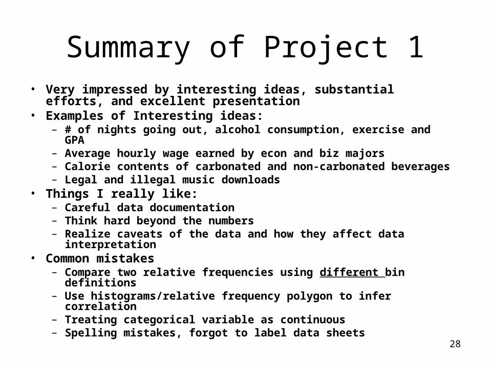
Summary of Project 1• Very impressed by interesting ideas, substantial efforts, and
excellent presentation• Examples of Interesting ideas:
– # of nights going out, alcohol consumption, exercise and GPA– Average hourly wage earned by econ and biz majors– Calorie contents of carbonated and non-carbonated beverages– Legal and illegal music downloads
• Things I really like: – Careful data documentation– Think hard beyond the numbers– Realize caveats of the data and how they affect data
interpretation• Common mistakes
– Compare two relative frequencies using different bin definitions– Use histograms/relative frequency polygon to infer correlation– Treating categorical variable as continuous– Spelling mistakes, forgot to label data sheets

29
Class 6-7: Probability Theory(e.stat Chapters 5 and 6)
• Population: entire set of events that occur in a given universe.– Event probability– Probability density function (PDF, )– Cumulative density function (CDF, )– Population statistics (mean, variance, etc.)– Certainty about a random process
• Sample: a subset of a population– Data analysis– Random by nature– Sample statistics are random variables, but population
statistics are not!
f x( )
F x( )
30
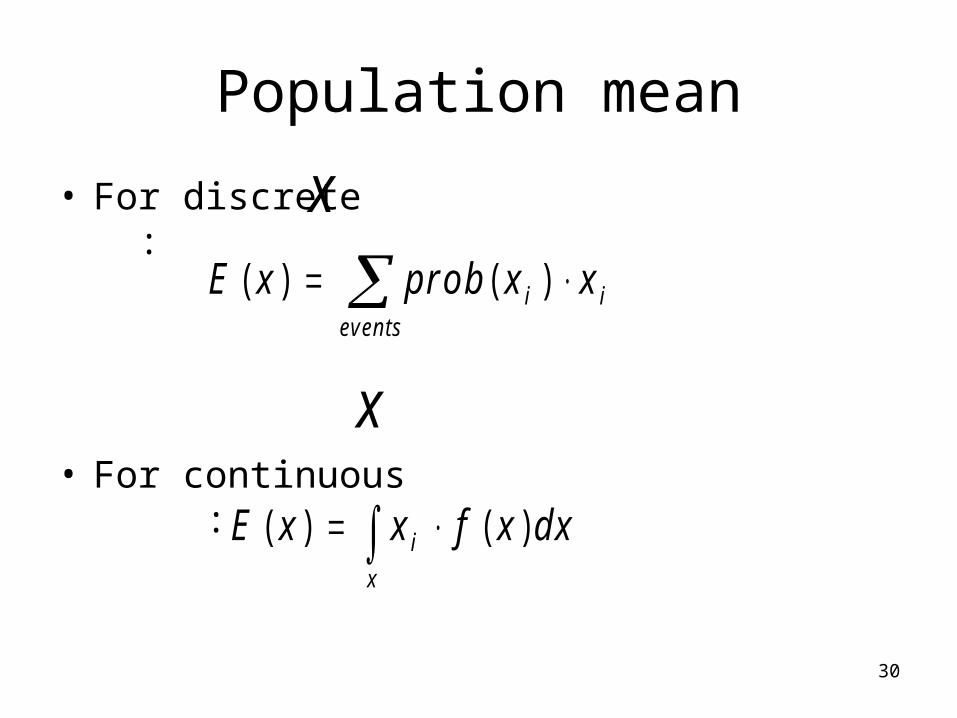
Population mean
• For discrete :
• For continuous :
E x prob x xi ieven ts
( ) ( ) x
x
E x x f x dxi
x
( ) ( )

31
Population variance and standard deviation
• For discrete :
• For continuous :
2 2 prob x x E xieven ts
( ) ( ( ))
x
x
2 2 ( ( )) ( )x E x f x dxx
32
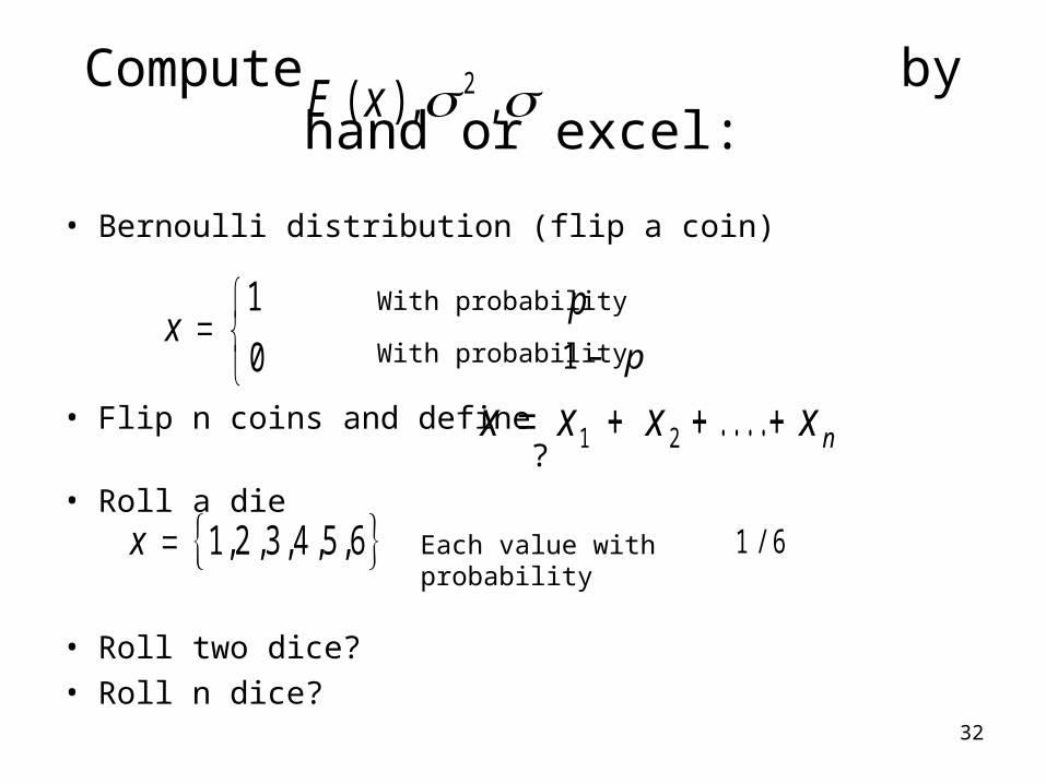
Compute by hand or excel:
• Bernoulli distribution (flip a coin)
• Flip n coins and define ?• Roll a die
• Roll two dice?• Roll n dice?
E x( ), , 2
x
1
0
With probability pWith probability 1 p
Each value with probability 1 6/ x 1 2 3 4 5 6, , , , ,
x x x x n 1 2 . . . .
33
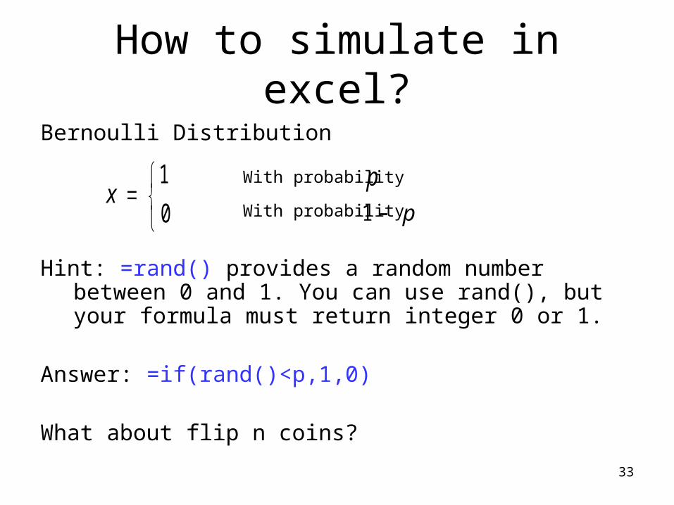
How to simulate in excel?
Bernoulli Distribution
Hint: =rand() provides a random number between 0 and 1. You can use rand(), but your formula must return integer 0 or 1.
Answer: =if(rand()<p,1,0)
What about flip n coins?
x
1
0
With probability pWith probability 1 p

34
How to simulate in excel?
Roll a die
Hint: Your formula must return an integer between 1 and 6, with equal probability.
Answer: =round(rand()*6+0.5,0), or =randbetween(1,6)Note: randbetween function may not exist in some versions of Excel.
What about roll n dice?
Each value with probability 1 6/ x 1 2 3 4 5 6, , , , ,

35
Compute by hand or excel:
• uniform distribution between (a,b)
f xb a
( ) 1
E x( ), , 2
a b
x
1/(b-a)
Answer:
E xa b
b a
( )
( )
2
1 22
2

36
Normal distribution
• Normal distribution:
x N~ ( , ) prob x
prob x
prob x
( ) .
( ) .
( ) .
0 6 7
2 2 0 9 5
3 3 0 9 9
x N~ ( , )1 0 0 1 0
Normal PDF
0.000
0.250
0.500
0.750
1.000
70.0
80.0
90.0
100.0
110.0
120.0
130.0
x
f(x)
, cum
(p(x
))Example:

37
What about ?
E x x E x E x
Var x x Var x Var x Cov x x
x x Var x Var x Cov x x
( ) ( ) ( )
( ) ( ) ( ) ( , )
( ) ( ) ( ) ( , )
1 2 1 2
1 2 1 2 1 2
1 2 1 2 1 2
2
2
Note: if both x1 and x2 are normally distributed, so is x1+x2. But if x1 and x2 are uniformly distributed, x1+x2 is not uniformly distributed.
x x x 1 2
38
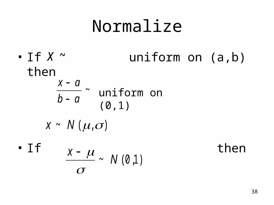
Normalize
• If uniform on (a,b) then
• If then
x a
b a
~ uniform on (0,1)
x N~ ( , )
xN
~ ( , )0 1
x ~
39
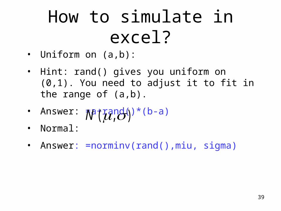
How to simulate in excel?
• Uniform on (a,b):
• Hint: rand() gives you uniform on (0,1). You need to adjust it to fit in the range of (a,b).
• Answer: =a+rand()*(b-a)
• Normal:
• Answer: =norminv(rand(),miu, sigma)
N ( , )
40
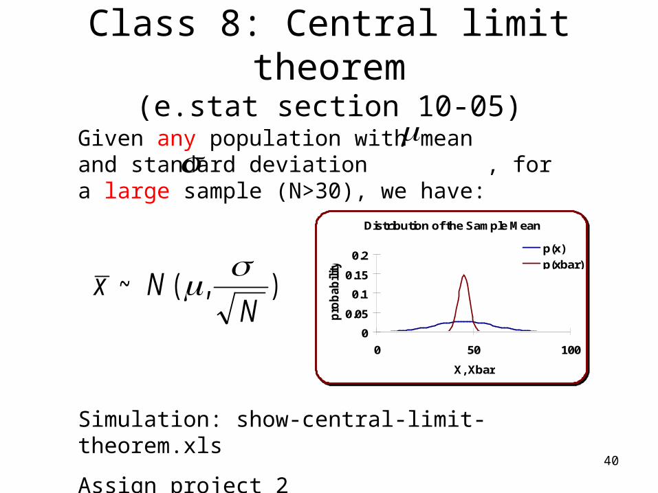
Class 8: Central limit theorem(e.stat section 10-05)
x NN
~ ( , )
Given any population with mean and standard deviation , for a large sample (N>30), we have:
Simulation: show-central-limit-theorem.xls
Assign project 2
Distribution of the Sample Mean
0
0.05
0.1
0.15
0.2
0 50 100
X, Xbar
pro
bab
ility
p(x)p(xbar)

41
Show CLT in Excel (1)
• Choose a population– type of distribution, e.g. Bernoulli– distribution parameters, e.g. p=0.3.
• Simulate data – 200 samples– each sample of size N
• Lock in the simulated data so the samples do not change later on – copy, paste special

42
Show CLT in Excel (2)
• Calculate sample mean for each sample
• Compare the distributions of (1) all the raw data and (2) all the sample means– bin range must be wide enough to cover the
most dispersed distribution– bin width must be narrow enough so that
there are at least 4-5 bins for the most concentrated distribution

43
Summary of project 2
• Most students perform well
• Correct answer:
Relative Frequency Polygon (Uniform)
0
0.05
0.1
0.15
0.2
0.25
0.3
0.35
0.4
0 8 16 24 32 40 48 56 64 72 80 88 96
Bins
relative frequency for n=20
relative frequency for n=30
relative frequency for n=40
relative frequency forrawdata
Relative Frequency Polygon
0
0.1
0.2
0.3
32 35 38 41 44 47 50 53 56 59 62 65 68
Bins
relative frequency for n=20
relative frequency for n=30
relative frequency for n=40
relative frequency forrawdata

44
Common mistakes in project 2
• You should simulate from normal/uniform distribution, not from Bernoulli.
• You should put raw data and sample mean in ONE relative frequency polygon. To do so, you must have the same bin definition for all the data series plotted in the graph.
45
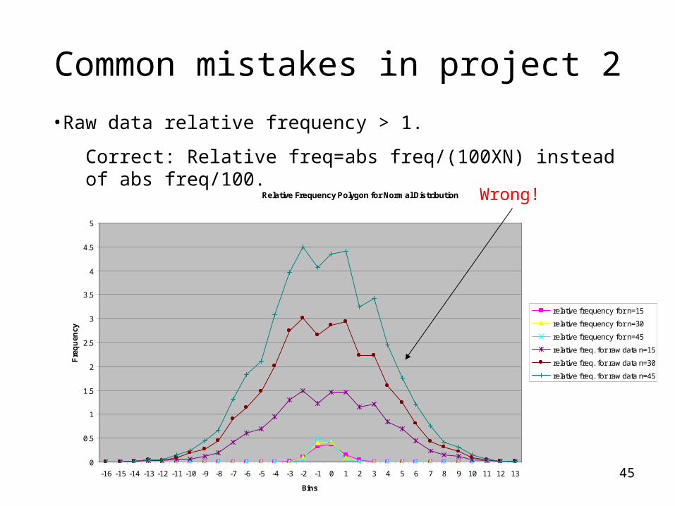
Common mistakes in project 2
•Raw data relative frequency > 1.
Correct: Relative freq=abs freq/(100XN) instead of abs freq/100.
Relative Frequency Polygon for Normal Distribution
0
0.5
1
1.5
2
2.5
3
3.5
4
4.5
5
-16 -15 -14 -13 -12 -11 -10 -9 -8 -7 -6 -5 -4 -3 -2 -1 0 1 2 3 4 5 6 7 8 9 10 11 12 13
Bins
Fre
qu
ency
relative frequency for n=15
relative frequency for n=30
relative frequency for n=45
relative freq. for raw data n=15
relative freq. for raw data n=30
relative freq. for raw data n=45
Wrong!
46
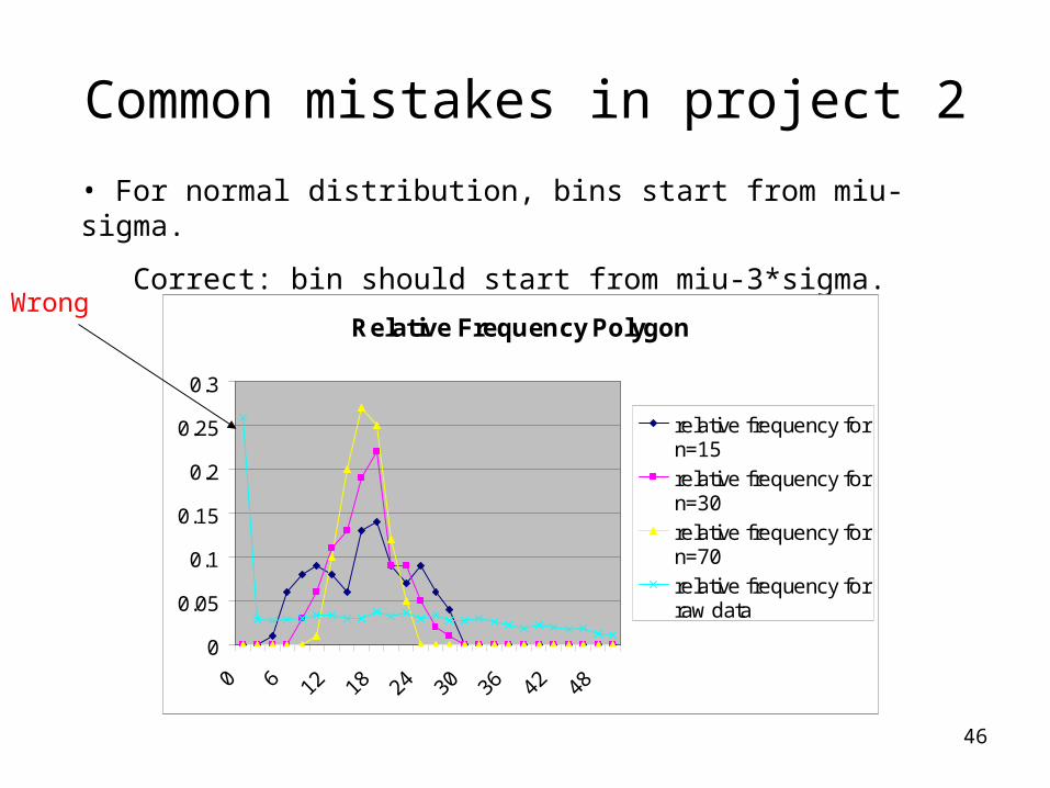
Common mistakes in project 2
• For normal distribution, bins start from miu-sigma.
Correct: bin should start from miu-3*sigma.
Relative Frequency Polygon
0
0.05
0.1
0.15
0.2
0.25
0.3
0 6 12 18 24 30 36 42 48
relative frequency forn=15
relative frequency forn=30
relative frequency forn=70
relative frequency forraw data
Wrong

47
Class 9: Mean estimation
• According to CLT, sample mean is an unbiased estimate of population mean, but with some errors.
• What is the distribution of if
?
Answer:
xE x N( ) , , 0 1 0 1 0 0
x N E xN
N~ ( ( ), ) ( , )
0 1

48
distribution of sample mean (xbar)with E(x)=0
0
0.2
0.4
-3 -2.2 -1.4 -0.6 0.2 1 1.8 2.6
xbar
95% chance within this range
E xN
( ) 2 E x
N( )
2
49
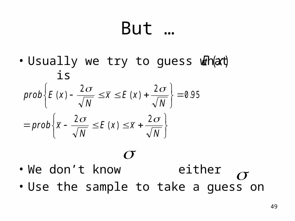
But …
• Usually we try to guess what is
• We don’t know either
• Use the sample to take a guess on
E x( )
prob E xN
x E xN
prob xN
E x xN
( ) ( ) .
( )
2 20 9 5
2 2
50
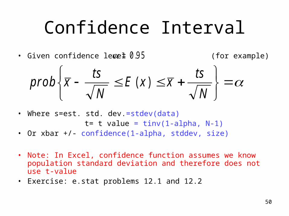
Confidence Interval
• Given confidence level (for example)
• Where s=est. std. dev.=stdev(data) t= t value = tinv(1-alpha, N-1)• Or xbar +/- confidence(1-alpha, stddev, size)
• Note: In Excel, confidence function assumes we know population standard deviation and therefore does not use t-value
• Exercise: e.stat problems 12.1 and 12.2
prob xts
NE x x
ts
N
( )
0 9 5.
51
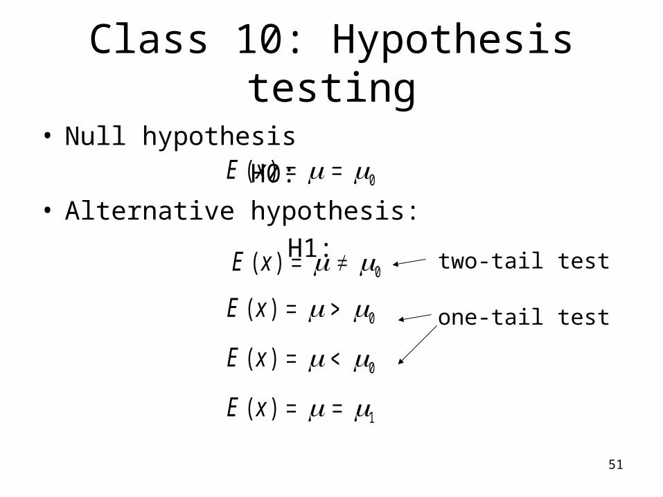
Class 10: Hypothesis testing
• Null hypothesis
H0: • Alternative hypothesis:
H1:
E x( ) 0
E x( ) 0
E x( ) 0
E x( ) 1
E x( ) 0
two-tail test
one-tail test
52
Logic
• Assume H0 is right
• Choose a confidence level
• Compute prob(get the sample mean)
• Reject H0 if prob(..) is too small, otherwise accept H0
0 9 5.
53
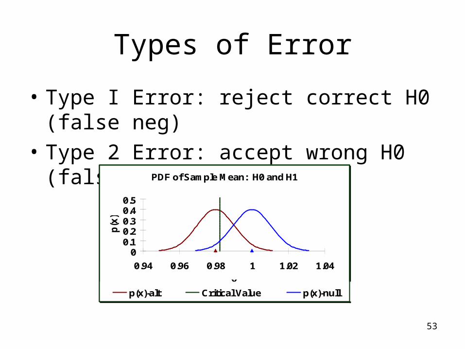
Types of Error
• Type I Error: reject correct H0 (false neg)
• Type 2 Error: accept wrong H0 (false pos)
PDF of Sample Mean: H0 and H1
00.10.20.30.40.5
0.94 0.96 0.98 1 1.02 1.04
x
p(x
)
p(x)-alt Critical Value p(x)-null mu's
54
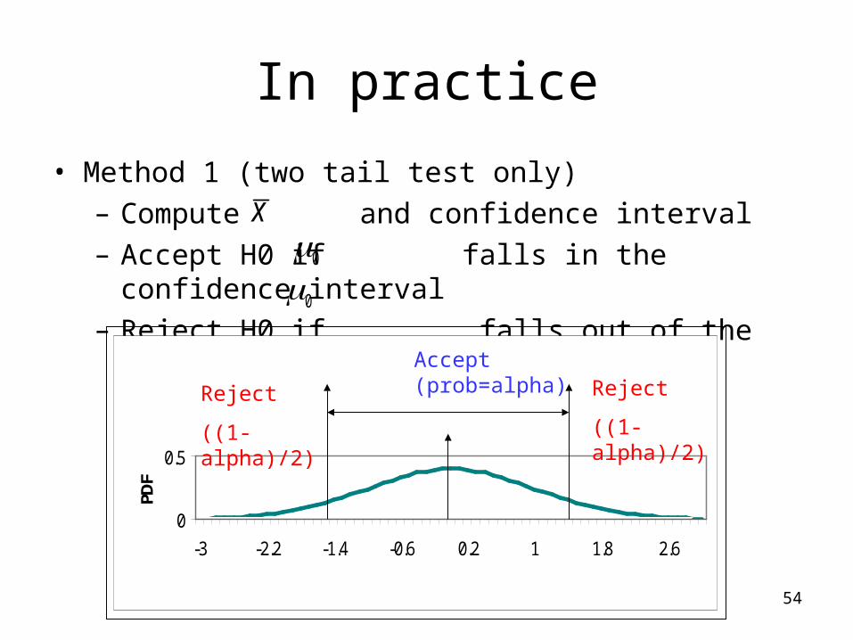
In practice
• Method 1 (two tail test only)– Compute and confidence interval– Accept H0 if falls in the confidence interval– Reject H0 if falls out of the confidence interval
x0
0
x
0
0.5
-3 -2.2 -1.4 -0.6 0.2 1 1.8 2.6
Accept (prob=alpha)Reject
((1-alpha)/2)
Reject
((1-alpha)/2)
55
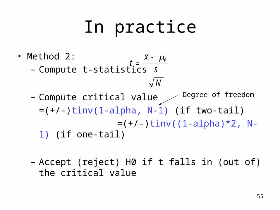
In practice
• Method 2:– Compute t-statistics
– Compute critical value
=(+/-)tinv(1-alpha, N-1) (if two-tail)
=(+/-)tinv((1-alpha)*2, N-1) (if one-tail)
– Accept (reject) H0 if t falls in (out of) the critical value
txs
N
0
Degree of freedom

56
0
0.5
-3 -2.2 -1.4 -0.6 0.2 1 1.8 2.6
Accept (prob=alpha)Reject
((1-alpha)/2)
Reject
((1-alpha)/2)t
Two-tail critical values
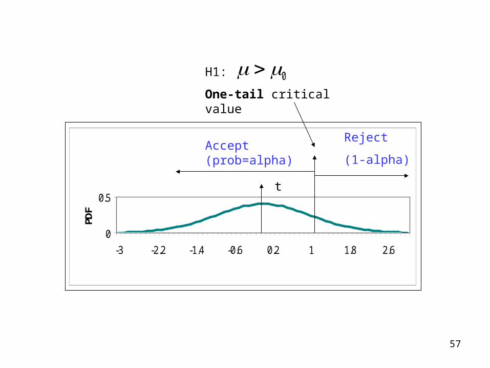
57
0
0.5
-3 -2.2 -1.4 -0.6 0.2 1 1.8 2.6
Accept (prob=alpha)
Reject
(1-alpha)
t
H1:
One-tail critical value
0

58
In practice
• Method 3:– Compute t-statistics
– Compute p-value = prob(t-stat>=|t|)=tdist(|t|, N-1,2) (if two-tail)
=tdist(|t|,N-1,1) (if one-tail)
– Reject H0 if p-value<(1-alpha)
Accept H0 if p-value>(1-alpha)
txs
N
0
59
Exercise
• What is H0? What is H1?
• Two-tail or one-tail?
• Choose a method
• E.stat problems: – two-tail test: e.stat 13.13 and 13.17– One-tail test: e.stat 13.20 and 13.E10

60
Two-tail vs. one-tail
• Two-tail test does not indicate which direction to go if we reject H0: , so the alternative is H1: .
• One-tail test has a strong view of one direction. For example, a saleman wants to know whether sales have increased from the past, in which case the alternative is H1: . If he is worried if the sales have decreased, the alternative will point to another direction where H1 is .
0
0
0
0

61
In Excel (alpha=95%):Two-tail• H0:
• H1:
• T-stat:
• Crit.Val:
(+/-) tinv(0.05,N-1)
• Reject if
t > + crit. val.
or t< - crit. val
One-tail• H0:
• H1:
• T-stat:
• Crit. Val:
= -tinv(0.10,N-1)
• Reject if
t<crit. val.
0
One-tail• H0:
• H1:
• T-stat:
• Crit. Val
= + tinv(0.10,N-1)
• Reject if
t> crit. val.
0
x
s N
0
/
x
s N
0
/
x
s N
0
/
0
0
0 0

62
Three methods, same resultTwo-tail• H0:
• H1:
• T-stat:
• Crit.Val:
(+/-) tinv(0.05,N-1)
• Reject if
t > + crit. val.
or t< - crit. val
0
x
s N
0
/
0
Two-tail• H0:
• H1:
• T-stat:
• P-value:
tdist(|t-stat|,N-1,2)
• Reject if
p<0.05
0
x
s N
0
/
0
Two-tail• H0:
• H1:
• Conf. Interval
[ ,
]
tinv(0.05,N-1)
• Reject if
is out of conf. interval
0
0
x ts N /
x ts N /
0

63
Class 11: two sample testing
• One sample test H0:
• What if we don’t know but have two samples
• Can we compare and ?
• Yes, must account for errors in both
0
0
x 1 x 2

64
Two independent samples
• H0:• H1: (two-tail) (one-tail)• Independent errors in the two samples are
independent
• Degree of freedom [min(N1,N2)-1]• Exercise: e.stat problems 14.5, 14.6
1 2 1 2
1 2
tx x
s
N
s
N
( ) ( )1 2 1 2
12
1
22
2

65
Two matched samples(same subjects, N1=N2)
• H0:• H1: (two-tail) (one-tail)• Generate a new variable dx=x1-x2• Transform H0: • Now is a one-sample test• Degree of freedom N1-1• Example: e.stat figure 14.8• Exercise: e.stat problem 14.7
1 2 1 2
1 2
dx 1 2
66
How to tell if two samples are matched or not?
• N1=N2 for matched pairs
• Same subjects?
• If resorting one sample does not affect the comparison, they are independent

67
Class 12: regression
• “Regress Y on X” means:
y x Dependent variable
Independent variable(s)
coefficients
Error term
68
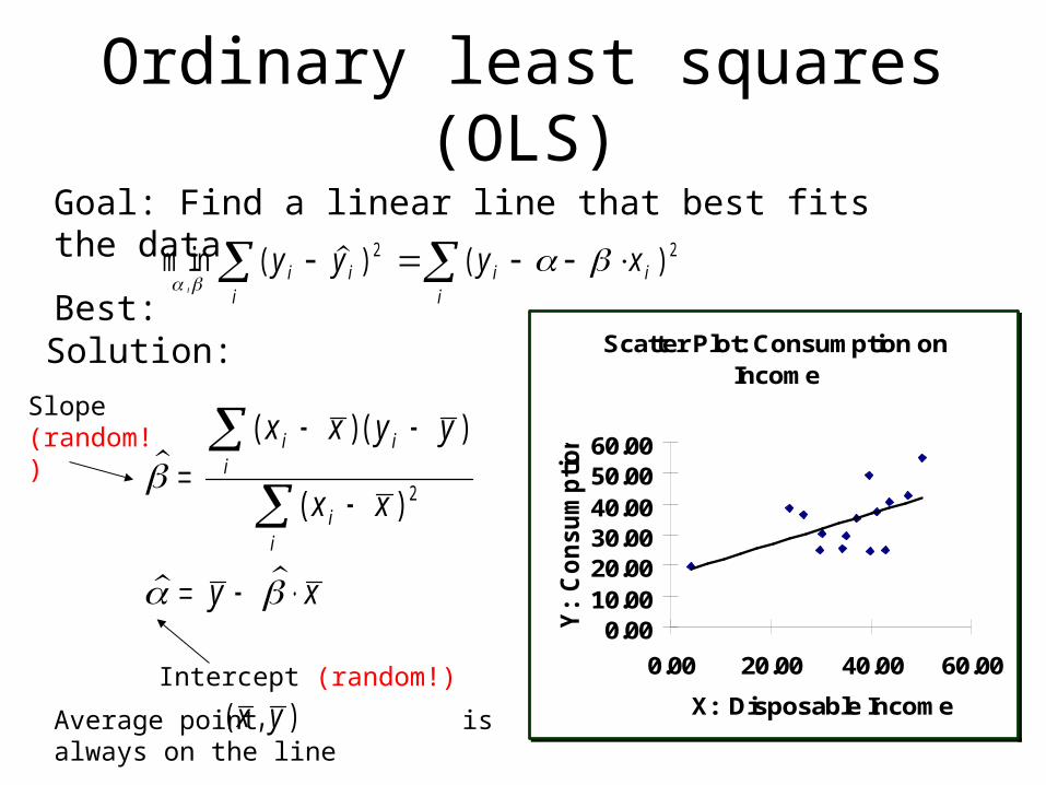
Ordinary least squares (OLS)
Scatter Plot: Consumption on Income
0.0010.0020.0030.0040.0050.0060.00
0.00 20.00 40.00 60.00
X: Disposable Income
Y:
Consu
mptio
n
Goal: Find a linear line that best fits the data
Best: m in ( ) ( ),
y y y xi ii
i ii
2 2
Intercept (random!)
Slope (random!)
Average point is always on the line
( , )x y
( )( )
( )
x x y y
x x
y x
i ii
ii
2
Solution:
69
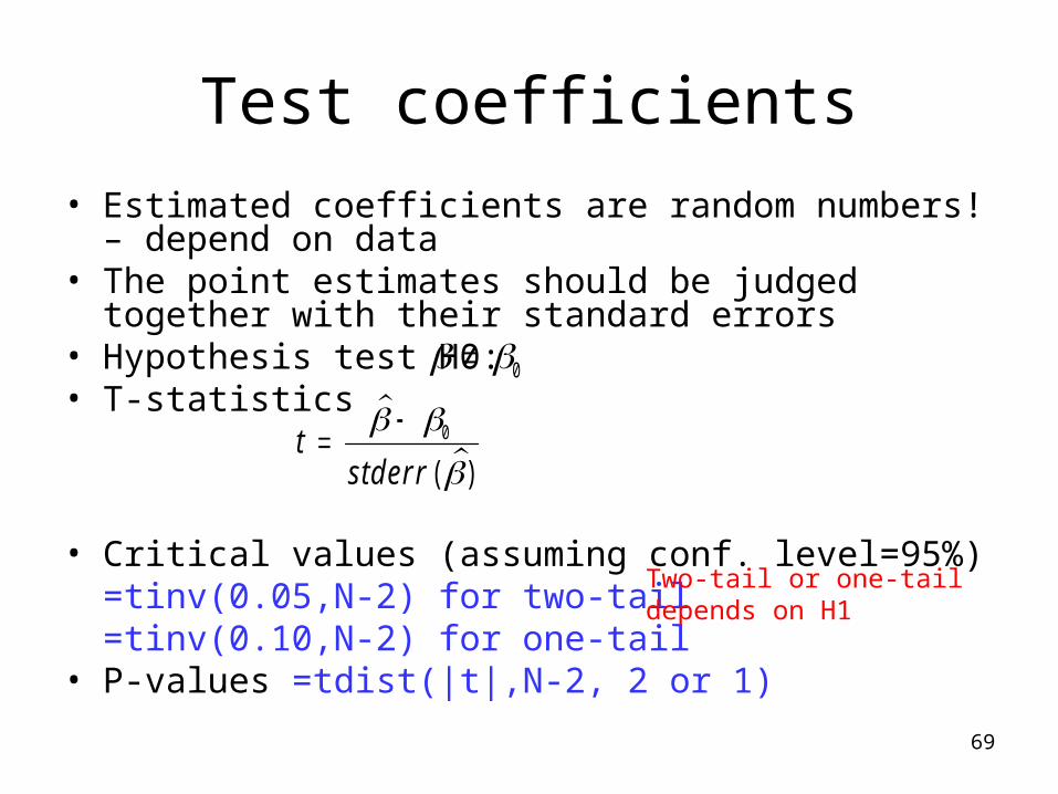
Test coefficients
• Estimated coefficients are random numbers! – depend on data
• The point estimates should be judged together with their standard errors
• Hypothesis test H0: • T-statistics
• Critical values (assuming conf. level=95%)=tinv(0.05,N-2) for two-tail=tinv(0.10,N-2) for one-tail
• P-values =tdist(|t|,N-2, 2 or 1)
0
tstderr
( )
0
Two-tail or one-tail depends on H1

70
Measure the fit of OLS
• Total sum of squared deviations (TSS):
• Decompose TSS:– Explained by the model:– Unexplained residuals:
• R-square: (explained)/(total)
( )y yi
2
( )y yi
2
( )y yi
2
71
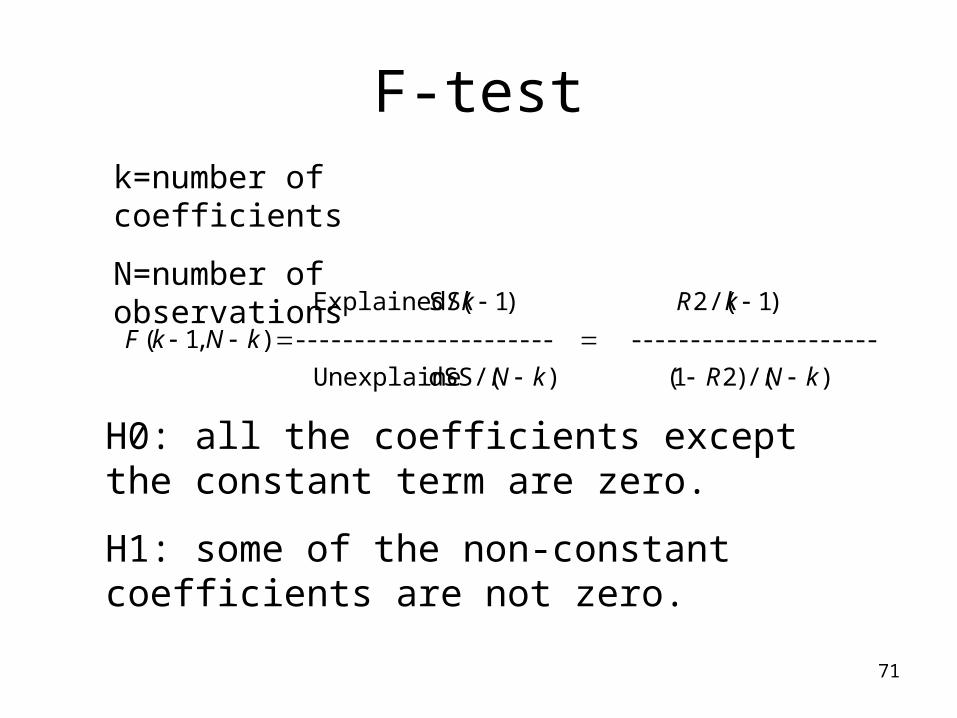
F-testk=number of coefficients
N=number of observations
H0: all the coefficients except the constant term are zero.
H1: some of the non-constant coefficients are not zero.
)/()21( )/( dSSUnexplaine
--------------------- ---------------------- ),1(
)1/(2 )1/(SExplainedS
kNRkN
kNkF
kRk
72
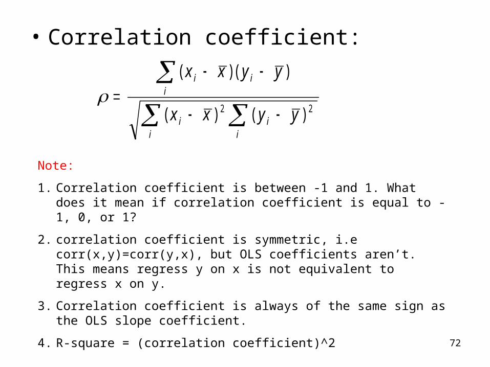
• Correlation coefficient:
( )( )
( ) ( )
x x y y
x x y y
i ii
i iii
2 2
Note:
1. Correlation coefficient is between -1 and 1. What does it mean if correlation coefficient is equal to -1, 0, or 1?
2. correlation coefficient is symmetric, i.e corr(x,y)=corr(y,x), but OLS coefficients aren’t. This means regress y on x is not equivalent to regress x on y.
3. Correlation coefficient is always of the same sign as the OLS slope coefficient.
4. R-square = (correlation coefficient)^2
73
Regression in Excel
• Method 1:=linest(data of y, data of x, include const?, other statistics?)No output labels, must be familiar with the output layout
• Method 2: Tools - data analysis – regression
• Note: you could have multiple x, but they must be adjacent to each other.
• Example: e.stat Figure 19.7• Exercise: e.stat problems 19.E1, 19.E2, 19.E3

74
Assumptions and Caveats in OLS(e.stat section 22-04)
• Errors have mean zero.
• Errors have a constant standard deviation.
• Errors are drawn independently.
• Errors are uncorrelated with x. All the important x are included in the regression.(omitted variable bias, see e.stat Figure 22.4.)
• Errors are distributed normally.
75
Class 14: Midterm Review
– open book– understand the concepts– use them in real examples– 9:30-10:45am, Plant Sciences 1129– If you cannot attend the midterm for reasons
that are consistent with University Policy, please let me know AT LEAST 12 hours BEFORE the midterm time, otherwise your midterm grade will be counted as zero.
76
Concepts to grasp (1)
• Population / sample• Population
– Cdf (prob(var<x))– Pdf (first derivative of cdf)– population mean, population std. dev.
• Sample– Histogram, frequency polygon, quartiles, percentiles, sample
mean, sample std. dev., skewness, kurtosis
• Population sample – Central limit theorem xbar~N(µ, σ/sqrt(n))
• Sample Population – Xbar is a proxy of µ with noise

77
Concepts to grasp (2)
• Inference– Type I error, Type II error– Confidence level α– Confidence interval– Hypothesis testing
• H0• H1• Accept/reject?• One-tail, two-tail test
78
Summary of Excel (1)
• Basic excel – open, save and close files– cut, paste and paste special– change format for cell, row or columns– sort data by one or two variables– chart wizard– freeze panes– drag cells– use excel functions
79
Summary of Excel (2)
• Data description – mean, median, trimmed mean– standard deviation, variance– quartiles– mode, skewness, kurtosis– histogram (absolute frequency)– relative frequency polygon
80
Summary of Excel (3)
• Probability theory – PDF, CDF– mean and standard deviation– bernoulli, binomial– uniform, normal– how to simulate them in Excel?– Central limit theorem– how to see central limit theorem in excel?
81
Summary of Excel (4)
• Estimation and Hypothesis testing– use sample mean to estimate population mean– confidence interval– type I error and type II error– null hypothesis (H0) and alternative hypothesis (H1)– one-tail vs. two-tail– t-statistics, critical value, p-value– one-sample test – two-sample test (independent)– two-sample test (matched pair)
82
Summary of Excel (5)• Linear regression
– model• one variable on the right hand side• more than one variables on the right hand side• create and use binary variables
– fit of the model• R square• F test• scatter plot• correlation coefficient
– coefficient estimates• point estimate• hypothesis testing• omitted variable bias

83
Class 15: Midterm Grades


![THE GINGER GUIDE · PDF file · 2017-09-27GINGER GUIDE THE [ORIGINS OF FLAVOR ] ... omes of ginger ingiber officinale) ... ORGANIC GINGER SYRUP #25400 INGREDIENTS: Organic ginger,](https://static.fdocuments.in/doc/165x107/5aadf2a57f8b9a22118b6437/the-ginger-guide-guide-the-origins-of-flavor-omes-of-ginger-ingiber-officinale.jpg)
