1 Non-Seasonal Box-Jenkins Models. 2 Box-Jenkins (ARIMA) Models The Box-Jenkins methodology refers...
75
1 Non-Seasonal Box- Jenkins Models
-
Upload
moses-johns -
Category
Documents
-
view
223 -
download
4
Transcript of 1 Non-Seasonal Box-Jenkins Models. 2 Box-Jenkins (ARIMA) Models The Box-Jenkins methodology refers...

1
Non-Seasonal Box-Jenkins Models

2
Box-Jenkins (ARIMA) Models
The Box-Jenkins methodology refers to a set of procedures for identifying and estimating time series models within the class of autoregressive integrated moving average (ARIMA) models.
ARIMA models are regression models that use lagged values of the dependent variable and/or random disturbance term as explanatory variables.
ARIMA models rely heavily on the autocorrelation pattern in the data
This method applies to both non-seasonal and seasonal data. In this course, we will only deal with non-seasonal data.

3
Box-Jenkins (ARIMA) Models
Three basic ARIMA models for a stationary time series yt :
(1) Autoregressive model of order p (AR(p))
i.e., yt depends on its p previous values
(2) Moving Average model of order q (MA(q))
i.e., yt depends on q previous random error terms
,2211 tptpttt yyyy
,2211 qtqtttty

4
Box-Jenkins (ARIMA) Models
(3) Autoregressive-moving average model of order p and q (ARMA(p,q))
i.e., yt depends on its p previous values and q previous random error terms
,2211
2211
qtqttt
ptpttt yyyy

5
Box-Jenkins (ARIMA) Models
In an ARIMA model, the random disturbance term
is typically assumed to be “white noise”; i.e., it is identically and independently distributed with a mean of 0 and a common variance across all observations.
We write ~ i.i.d.(0, )
t
2
t 2
6
A five-step iterative procedure
1) Stationarity Checking and Differencing
2) Model Identification
3) Parameter Estimation
4) Diagnostic Checking
5) Forecasting

7
Step One: Stationarity checking

8
Stationarity
“Stationarity” is a fundamental property underlying almost all time series statistical models.
A time series yt is said to be stationary if it satisfies the following conditions:
2 2
(1) ( ) .
(2) ( ) [( ) ] .
(3) ( , ) .
t y
t t y y
t t k k
E y u for all t
Var y E y u for all t
Cov y y for all t

9
Stationarity
The white noise series satisfies the stationarity condition because
(1) E( ) = 0
(2) Var( ) =
(3) Cov( ) = for all s 0
t
2
t
t
t t s

10
Example of a white noise series
3632282420161284
100
80
60
40
20
0
Time
Time Series Plot

11
Example of a non-stationary series
2902612322031741451168758291
4000
3900
3800
3700
3600
3500
Time
Time Series Plot of Dow-Jones Index

12
Stationarity
Suppose yt follows an AR(1) process without drift.
Is yt stationarity?
Note that
ot
tttt
ttt
ttt
y
y
yy
133
122
111
1211
11
...........
)(
13
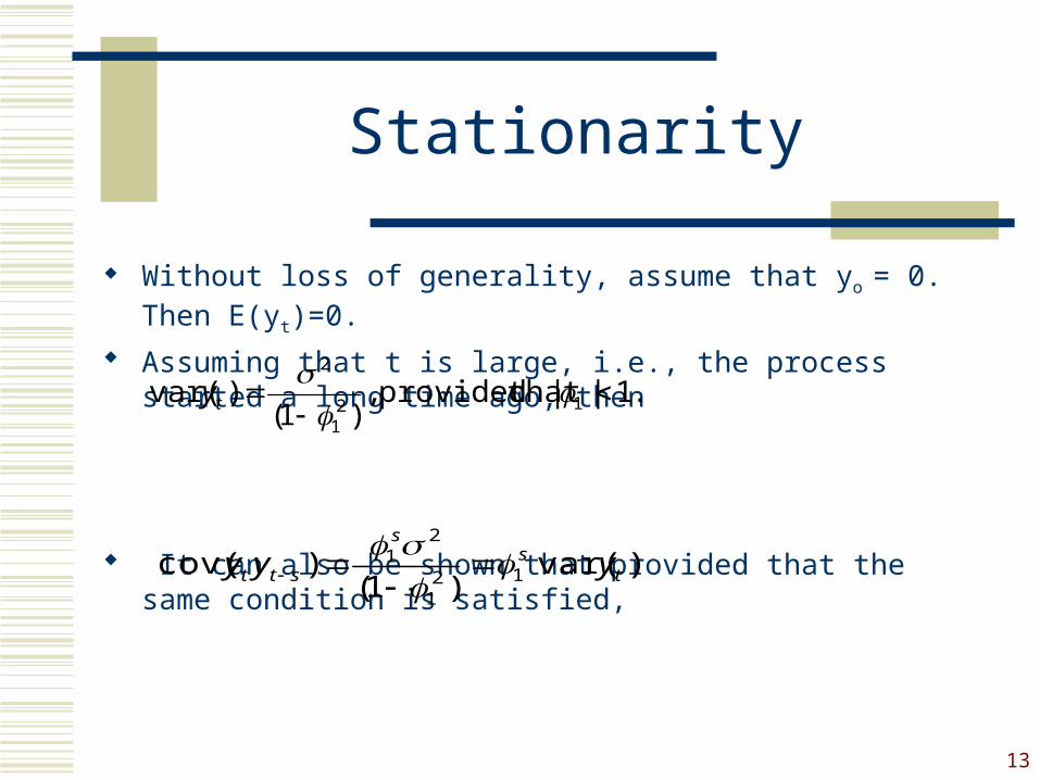
Stationarity
Without loss of generality, assume that yo = 0. Then E(yt)=0.
Assuming that t is large, i.e., the process started a long time ago, then
It can also be shown that provided that the same condition is satisfied,
.1|| that provided ,)1(
)var( 121
2
ty
)var()1(
)cov( 121
21
ts
s
stt yyy

14
Stationarity
Special Case: 1 = 1
It is a “random walk” process. Now,
Thus,
.1 ttt yy
1
0
.t
jjtty
2
2
(1) ( ) 0 .
(2) ( ) .
(3) ( , ) ( ) .
t
t
t t s
E y for all t
Var y t for all t
Cov y y t s for all t

15
Stationarity
Suppose the model is an AR(2) without drift, i.e.,
It can be shown that for yt to be stationary,
The key point is that AR processes are not stationary unless appropriate prior conditions are imposed on the parameters.
tttt yyy 2211
1 || and 1 ,1 21221
16
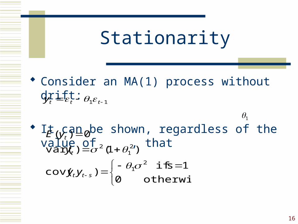
Stationarity
Consider an MA(1) process without drift:
It can be shown, regardless of the value of , that 11 ttty
otherwise 0
1s if )cov(
)1()var(
0)(
21
21
2
stt
t
t
yy
y
yE
1

17
Stationarity
For an MA(2) process
2211 tttty
otherwise 0
2 s if
1s if )1(
)cov(
)1()var(
0)(
22
22
1
22
21
2
stt
t
t
yy
y
yE

18
Stationarity
In general, MA processes are stationarity regardless of the values of the parameters, but not necessarily “invertible”.
An MA process is said to be invertible if it can be converted into a stationary AR process of infinite order.
The conditions of invertibility for an MA(k) process is analogous to those of stationarity for an AR(k) process. More on invertibility in tutorial.

19
Differencing
Often non-stationary series can be made stationary through differencing.
Examples:
stationary is7.0
but ,stationarynot is 7.07.1 )2
stationary is
but ,stationarynot is )1
11
21
1
1
ttttt
tttt
tttt
ttt
wyyw
yyy
yyw
yy

20
Differencing
Differencing continues until stationarity is achieved.
The differenced series has n-1 values after taking the first-difference, n-2 values after taking the second difference, and so on.
The number of times that the original series must be differenced in order to achieve stationarity is called the order of integration, denoted by d.
In practice, it is almost never necessary to go beyond second difference, because real data generally involve only first or second level non-stationarity.
1t t ty y y 2
1 1 2( ) ( ) 2t t t t t t ty y y y y y y

21
Differencing
Backward shift operator, B
B, operating on yt, has the effect of shifting the data back one period.
Two applications of B on yt shifts the data back two periods.
m applications of B on yt shifts the data back m periods.
1t tBy y
22( )t t tB By B y y
mt t mB y y
22
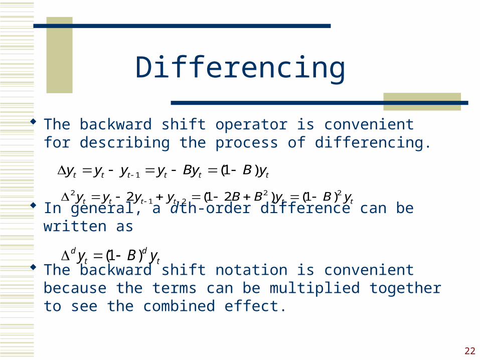
Differencing
The backward shift operator is convenient for describing the process of differencing.
In general, a dth-order difference can be written as
The backward shift notation is convenient because the terms can be multiplied together to see the combined effect.
1 (1 )t t t t t ty y y y By B y
2 2 21 22 (1 2 ) (1 )t t t t t ty y y y B B y B y
(1 )d dt ty B y

23
Population autocorrelation function
The question is, in practice, how can one tell if the data are stationary?
If the data are non-stationary (i.e., random walk), then = 1 for all values of k
If the data are stationary (i.e., ), then the magnitude of the autocorrelation coefficient “dies down” as k increases.
k. lagat t coefficienation autocorrel theis /
thatso )cov(Let
okk
kttk yy
k1k
process, AR(1)an Consider
1
1|| 1

24
Population autocorrelation function
Consider an AR(2) process without drift :
The autocorrelation coefficients are
.2211 tttt yyy
.2
1
,1
2211
2
21
22
2
11
kforkkk
25
Population autocorrelation function
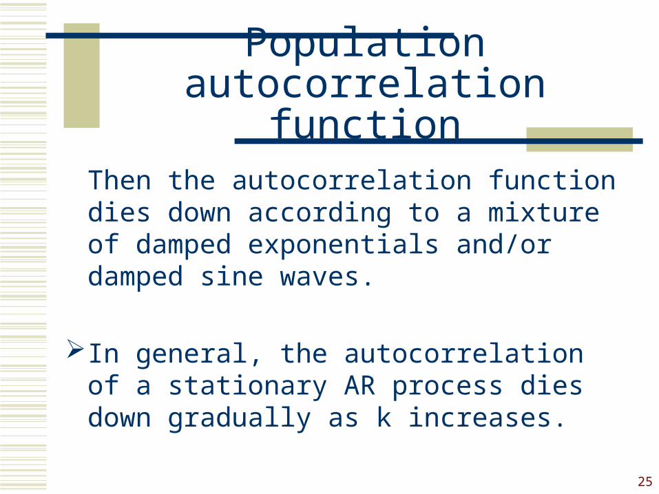
Then the autocorrelation function dies down according to a mixture of damped exponentials and/or damped sine waves.
In general, the autocorrelation of a stationary AR process dies down gradually as k increases.

26
Population autocorrelation function
Moving Average (MA) ProcessesConsider a MA(1) process without drift :
Recall that.11 ttty
.10
1),()3(
.)1())2(
.0)()1(
21
21
20
s
syyCov
tallforVar(y
tallforyE
sstt
t
t

27
Population autocorrelation function
Therefore the autocorrelation coefficient of the MA(1) process at lag k is
The autocorrelation function of the MA(1) process “cuts off” after lag k=1.
.10
11 2
1
1
0
k
k
kk
28
Population autocorrelation function
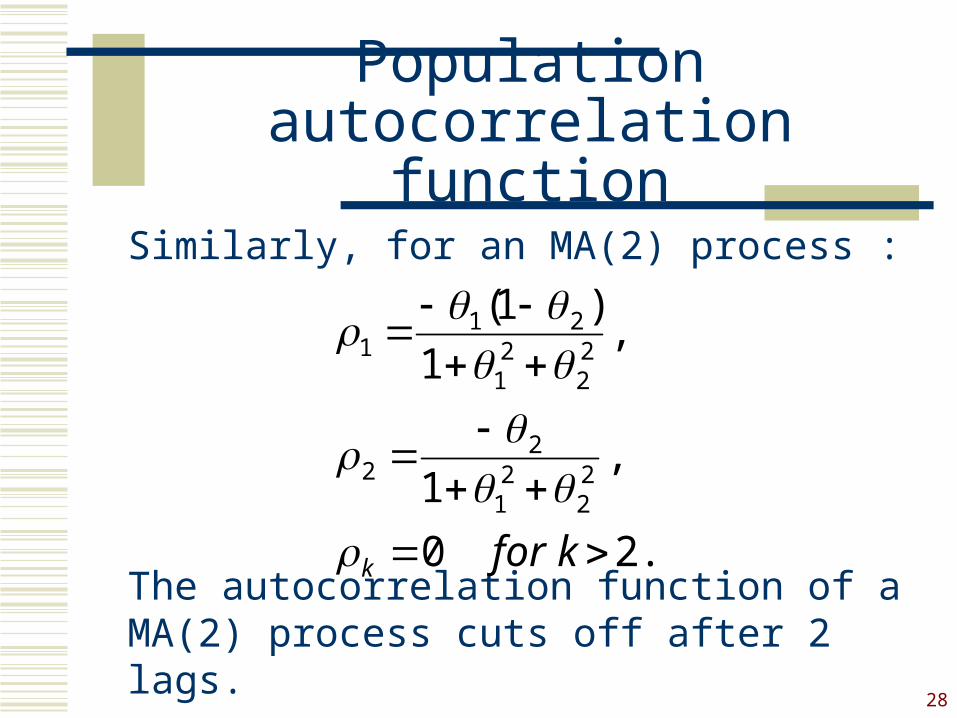
Similarly, for an MA(2) process :
The autocorrelation function of a MA(2) process cuts off after 2 lags.
.20
,1
,1
)1(
22
21
22
22
21
211
kfork

29
Population autocorrelation function
In general, all stationary AR processes exhibit autocorrelation patterns that “die down” to zero as k increases, while the autocorrelation coefficient of a non-stationary AR process is always 1 for all values of k. MA processes are always stationary with autocorrelation functions that cut off after certain lags.
Question: how are the autocorrelation coefficients “estimated” in practice?
30
Sample Autocorrelation Function (SAC)
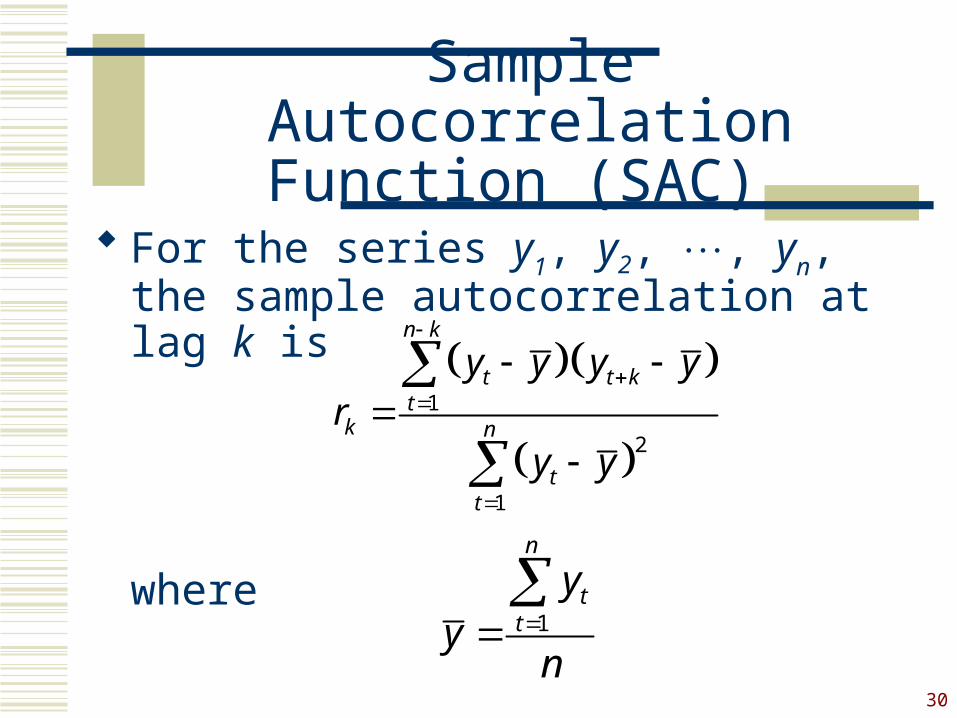
For the series y1, y2, , yn, the sample autocorrelation at lag k is
where
1
2
1
n k
t t kt
k n
tt
y y y yr
y y
1
n
tt
yy
n
31
Sample Autocorrelation Function (SAC)
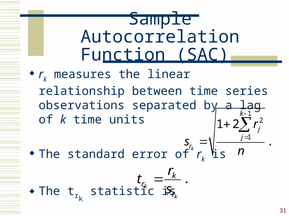
rk measures the linear relationship between
time series observations separated by a lag of k time units
The standard error of rk is
The trk statistic is
12
1
1 2
.k
k
jj
r
r
sn
.k
k
r
kr s
rt

32
Sample Autocorrelation Function (SAC)
Behaviour of SAC
(1) The SAC can cut off. A spike at lag k exists in the SAC if rk is statistically large. If
Then rk is considered to be statistically large. The SAC cuts off after lag k if there are no spikes at lags greater than k in the SAC.
2kr
t
33
Sample Autocorrelation Function (SAC)
(2) The SAC is said to die down if this function does not cut off but rather decreases in a
‘steady fashion’. The SAC can die down in(i) a damped exponential fashion(ii) a damped sine-wave fashion(iii) a fashion dominated by either one of
or a combination of both (i) and (ii).The SAC can die down fairly quickly or
extremely slowly.

34
Sample Autocorrelation Function (SAC)
The time series values y1, y2, …, yn should be considered stationary if the SAC of the time series values either cuts off fairly quickly or dies down fairly quickly.
However if the SAC of the time series values y1, y2, …, yn dies down extremely slowly, and r1 at lag 1 is close to 1, then the time series values should be considered non-stationary.

35
Stationarity Summary
Stationarity of data is a fundamental requirement for all time series analysis.
MA processes are always stationary AR and ARMA processes are generally not
stationary unless appropriate restrictions are imposed on the model parameters.

36
Stationarity Summary
Population autocorrelation function behaviour:
1) stationary AR and ARMA: dies down gradually as k increases
2) MA: cuts off after a certain lag
3) Random walk: autocorrelation remains at one for all values of k

37
Stationarity Summary
Sample autocorrelation function behaviour:1) stationary AR and ARMA: dies down gradually as k increases2) MA: cuts off after a certain lag3) Random walk: autocorrelation functions dies down very slowly and the estimated autocorrelation coefficient at lag 1 is close to 1.
What if the data are non-stationary? Perform differencing until stationarity is accomplished.

38
SAC of a stationary AR(1) process
The ARIMA Procedure Name of Variable = y
Mean of Working Series -0.08047 Standard Deviation 1.123515 Number of Observations 99
Autocorrelations
Lag Covariance Correlation -1 9 8 7 6 5 4 3 2 1 0 1 2 3 4 5 6 7 8 9 1 Std Error
0 1.262285 1.00000 | |********************| 0 1 0.643124 0.50949 | . |********** | 0.100504 2 0.435316 0.34486 | . |******* | 0.123875 3 0.266020 0.21075 | . |****. | 0.133221 4 0.111942 0.08868 | . |** . | 0.136547 5 0.109251 0.08655 | . |** . | 0.137127 6 0.012504 0.00991 | . | . | 0.137678 7 -0.040513 -.03209 | . *| . | 0.137685 8 -0.199299 -.15789 | . ***| . | 0.137761 9 -0.253309 -.20067 | . ****| . | 0.139576 "." marks two standard errors

39
SAC of an MA(2) process
The ARIMA Procedure Name of Variable = y
Mean of Working Series 0.020855 Standard Deviation 1.168993 Number of Observations 98
Autocorrelations
Lag Covariance Correlation -1 9 8 7 6 5 4 3 2 1 0 1 2 3 4 5 6 7 8 9 1 Std Error
0 1.366545 1.00000 | |********************| 0 1 -0.345078 -.25252 | *****| . | 0.101015 2 -0.288095 -.21082 | ****| . | 0.107263 3 -0.064644 -.04730 | . *| . | 0.111411 4 0.160680 0.11758 | . |** . | 0.111616 5 0.0060944 0.00446 | . | . | 0.112873 6 -0.117599 -.08606 | . **| . | 0.112875 7 -0.104943 -.07679 | . **| . | 0.113542 8 0.151050 0.11053 | . |** . | 0.114071 9 0.122021 0.08929 | . |** . | 0.115159
"." marks two standard errors

40
SAC of a random walk process
The ARIMA Procedure Name of Variable = y
Mean of Working Series 16.79147 Standard Deviation 9.39551 Number of Observations 98
Autocorrelations
Lag Covariance Correlation -1 9 8 7 6 5 4 3 2 1 0 1 2 3 4 5 6 7 8 9 1 Std Error
0 88.275614 1.00000 | |********************| 0 1 85.581769 0.96948 | . |******************* | 0.101015 2 81.637135 0.92480 | . |****************** | 0.171423 3 77.030769 0.87262 | . |***************** | 0.216425 4 72.573174 0.82212 | . |**************** | 0.249759 5 68.419227 0.77506 | . |**************** | 0.275995 6 64.688289 0.73280 | . |*************** | 0.297377 7 61.119745 0.69237 | . |************** | 0.315265 8 57.932253 0.65627 | . |************* | 0.330417 9 55.302847 0.62648 | . |*************. | 0.343460
"." marks two standard errors
41
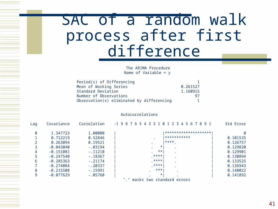
SAC of a random walk process after first difference
The ARIMA Procedure Name of Variable = y
Period(s) of Differencing 1 Mean of Working Series 0.261527 Standard Deviation 1.160915 Number of Observations 97 Observation(s) eliminated by differencing 1
Autocorrelations
Lag Covariance Correlation -1 9 8 7 6 5 4 3 2 1 0 1 2 3 4 5 6 7 8 9 1 Std Error
0 1.347723 1.00000 | |********************| 0 1 0.712219 0.52846 | . |*********** | 0.101535 2 0.263094 0.19521 | . |****. | 0.126757 3 -0.043040 -.03194 | . *| . | 0.129820 4 -0.151081 -.11210 | . **| . | 0.129901 5 -0.247540 -.18367 | .****| . | 0.130894 6 -0.285363 -.21174 | .****| . | 0.133525 7 -0.274084 -.20337 | .****| . | 0.136943 8 -0.215508 -.15991 | . ***| . | 0.140022 9 -0.077629 -.05760 | . *| . | 0.141892 "." marks two standard errors
42
Step Two: Model Identification
43
Model Identification
When the data are confirmed stationary, one may proceed to tentative identification of models through visual inspection of both the SAC and partial sample autocorrelation (PSAC) functions.

44
Partial autocorrelation function
Partial autocorrelations are used to measure the degree of association between Yt and Yt-k, when the effects of other time lags (1, 2, 3, …, k – 1) are removed.
The partial autocorrelations at lags 1, 2, 3, …, make up the partial autocorrelation function or PACF.
45
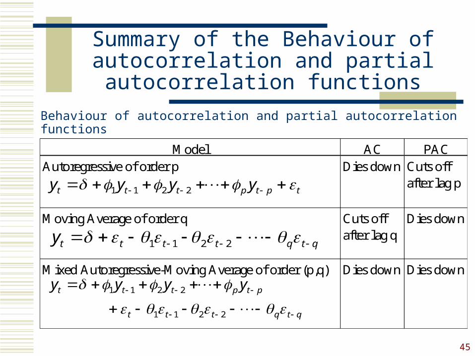
Summary of the Behaviour of autocorrelation and partial autocorrelation
functions
Behaviour of autocorrelation and partial autocorrelation functions
Model AC PAC
Dies down Dies down
Autoregressive of order p
Moving Average of order q
Mixed Autoregressive-Moving Average of order (p,q)
Dies down Cuts off after lag p
Cuts off after lag q
Dies down
1 1 2 2t t t p t p ty y y y
1 1 2 2t t t t q t qy
1 1 2 2
1 1 2 2
t t t p t p
t t t q t q
y y y y

46
Summary of the Behaviour of autocorrelation and partial autocorrelation
functions
Model AC PACFirst-order autoregressive
Second-order autoregressive
Dies down in a damped exponential fashion; specifically:
Cuts off after lag 1
Dies down according to a mixture of damped exponentials and/or damped sine waves; specifically:
Cuts off after lag 2
Behaviour of AC and PAC for specific non-seasonal models
11 k forkk
,1
,1
2
21
22
2
11
32211 k forkkk
1 1t t ty y
1 1 2 2t t t ty y y

47
Summary of the Behaviour of autocorrelation and partial autocorrelation
functions
Behaviour of AC and PAC for specific non-seasonal modelsModel AC PAC
First-order moving average
Second-order moving average
Cuts off after lag 1; specifically: Dies down in a fashion dominated by damped exponential decay
Cuts off after lag 2; specifically: Dies down according to a mixture of damped exponentials and/or damped sine waves
20
,1 2
1
11
k fork
.20
,1
,1
)1(
22
21
22
22
21
211
k fork
1 1t t ty
1 1 2 2t t t ty
48
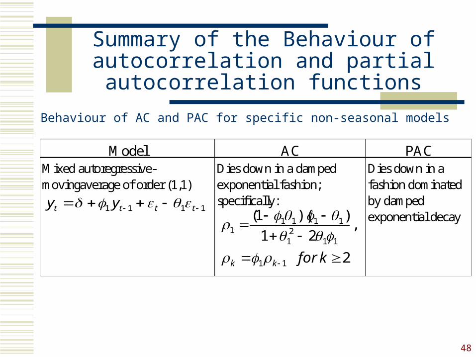
Summary of the Behaviour of autocorrelation and partial autocorrelation
functions
Behaviour of AC and PAC for specific non-seasonal models
Model AC PACMixed autoregressive-movingaverage of order (1,1)
Dies down in a damped exponential fashion; specifically:
Dies down in a fashion dominated by damped exponential decay
2
,21
))(1(
11
112
1
11111
k forkk
1 1 1 1t t t ty y
49
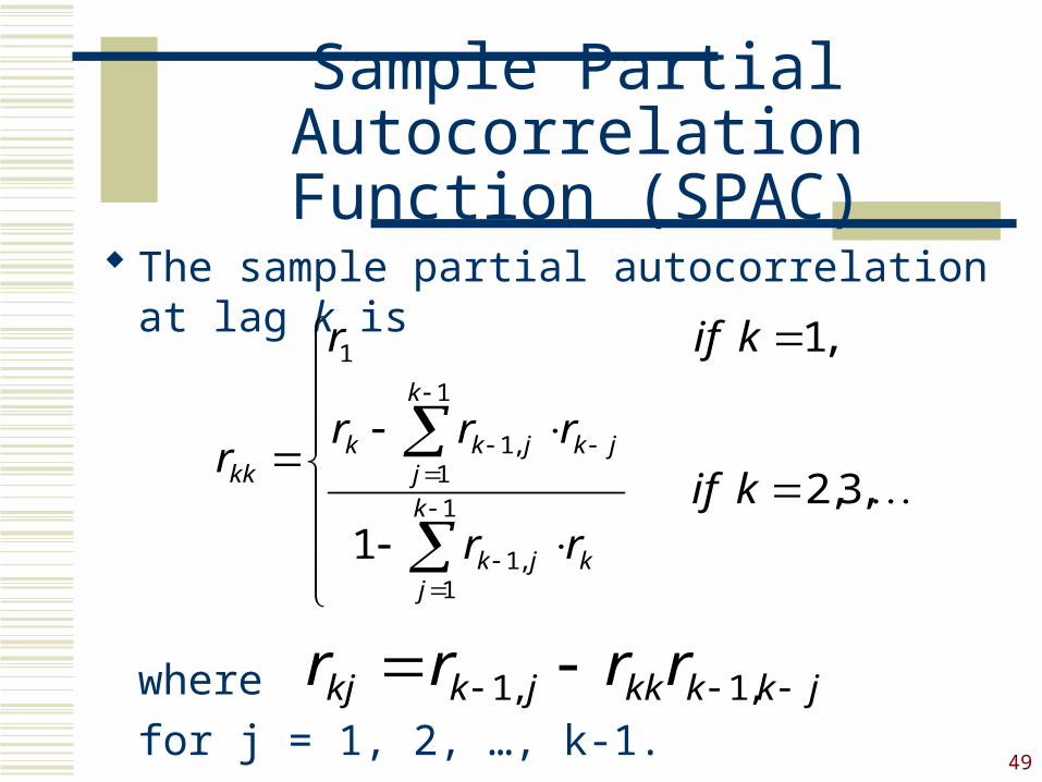
Sample Partial Autocorrelation Function (SPAC)
The sample partial autocorrelation at lag k is
where
for j = 1, 2, …, k-1.
,3,21
,1
1
1,1
1
1,1
1
k ifrr
rrr
k ifr
rk
jkjk
k
jjkjkk
kk
jkkkkjkkj rrrr ,1,1

50
Sample Partial Autocorrelation Function (SPAC)
rkk may intuitively be thought of as the sample autocorrelation of time series observations separated by a lag k time units with the effects of the intervening observations eliminated.
The standard error of rkk is
The trkk statistic is
1.
kkrsn
.kk
kk
r
kkr s
rt

51
Sample Partial Autocorrelation Function (SPAC)
Behaviour of SPAC similar to its of the SAC. The only difference is that rkk is considered to be statistically large if
for any k.2kkrt
52
Model Identification
Refers to class Examples 1, 2 and 3 for SAC and SPAC of simulated AR(2), MA(1) and ARMA(2,1) processes respectively.

53
Step Three: Parameter Estimation

54
Parameter Estimation
The method of least squares can be used. However, for models involving an MA component, there is no simple formula that can be applied to obtain the estimates.
Another method that is frequently used is maximum likelihood.

55
Parameter Estimation
Given n observations y1, y2, …, yn, the likelihood
function L is defined to be the probability of obtaining the data actually observed.
The maximum likelihood estimators (m.l.e.) are those value of the parameters for which the data actually observed are most likely, that is, the values that maximize the likelihood function L.

56
Parameter Estimation
Given n observations y1, y2, …, yn, the likelihood L is
the probability of obtaining the data actually observed.
For non-seasonal Box-Jenkins models, L is a function of , ’s, ’s and
2 given y1, y2, …, yn.
The maximum likelihood estimators (m.l.e.) are those values of the parameters which make the observation of the data a most likely event, that is, the values that maximize the likelihood function L.
57
Parameter Estimation
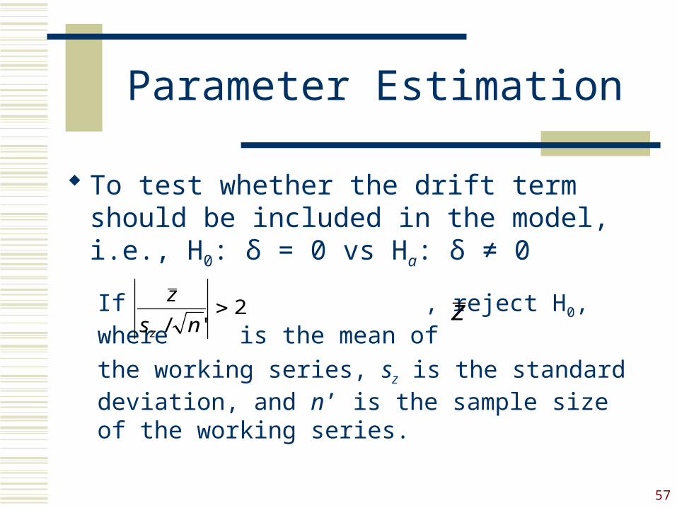
To test whether the drift term should be included in the model, i.e., H0: δ = 0 vs Ha: δ ≠ 0
If , reject H0, where is the mean of
the working series, sz is the standard deviation, and n’ is the sample size of the working series.
2'/
ns
z
z
z

58
Parameter estimation
Refers to the MA(1) example seen before The ARIMA Procedure Name of Variable = y
Mean of Working Series 0.020855 Standard Deviation 1.168993 Number of Observations 98
Here,
The drift term should not be included.
2 0.176608
)98/168993.1/(020855.0
t

59
Step Four: Diagnostic Checking
60
Diagnostic Checking
Often it is not straightforward to determine a single model that most adequately represents the data generating process, and it is not uncommon to estimate several models at the initial stage. The model that is finally chosen is the one considered best based on a set of diagnostic checking criteria. These criteria include
(1) t-tests for coefficient significance(2) residual analysis(3) model selection criteria

61
Diagnostic checking (t-tests)
Consider the data series of Example 4. First, the data appear to be stationary. Second, the drift term is significant. The SAC and SPAC functions indicate that the an AR(2) model probably best fits the data.
For illustration purpose, suppose an MA(1) and ARMA(2,1) are fiitted in addition to the AR(2).

62
Diagnostic checking (t-tests)
data MA2;input y;cards;4.04932687.08999114.7896497..2.22534772.439893;proc arima data=ma2;identify var=y;estimate p=2 method=ml printall;estimate q=1 method=ml printall;estimate p=2 q=1 method=ml printall;run;

63
Diagnostic checking (t-tests)
The AR(2) model estimation results produce
The t test statistic for is 8.93, indicating significance.
Similarly, the t test also indicates that is significantly different from zero.
21 49115.035039.068115.4ˆ ttt yyy
0: 1 oH
2
64
Diagnostic checking (t-tests)
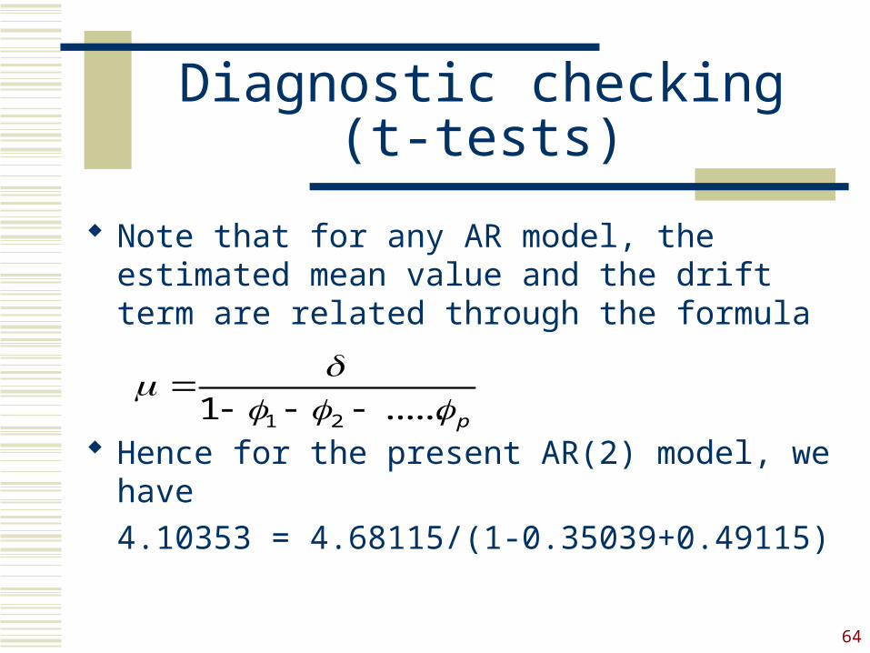
Note that for any AR model, the estimated mean value and the drift term are related through the formula
Hence for the present AR(2) model, we have
4.10353 = 4.68115/(1-0.35039+0.49115)
1 21 ...... p

65
Diagnostic checking (t-tests)
The MA(1) model produces
The t test indicates significance of the coefficient of .
Note that for any MA models,
148367.010209.4 ttt eey
1
.
66
Diagnostic checking (t-tests)
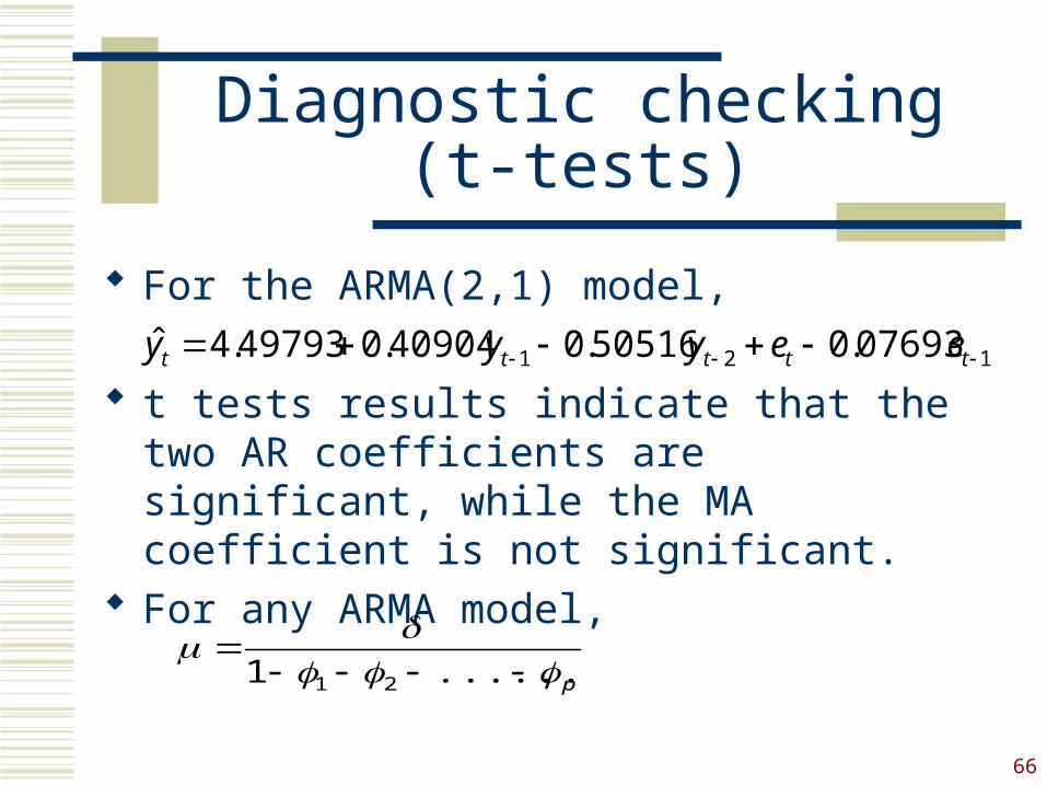
For the ARMA(2,1) model,
t tests results indicate that the two AR coefficients are significant, while the MA coefficient is not significant.
For any ARMA model,
121 07693.050516.040904.049793.4ˆ ttttt eeyyy
p
.......1 21

67
Residual Analysis
If an ARMA(p,q) model is an adequate representation of the data generating process, then the residuals should be uncorrelated.
Portmanteau test statistic:
2)(
1
2* ~
)()2)(()( qpk
k
l
l
ldn
erdndnkQ

68
Residual Analysis
Let’s take the AR(2) model as an example, let ut be the model’s residual. It is assumed that
Suppose we want to test, up to lag 6,
The portmanteau test statistic gives 3.85 with a p-value of 0.4268. Hence the null cannot be rejected and the residuals are uncorrelated at least up to lag 6.
0......: 621 oH
...........2211 ttt uuu

69
Residual Analysis
The results indicate that AR(2) and ARMA(2, 1) residuals are uncorrelated at least up to lag 30, while MA(1) residuals are correlated.

70
Model Selection Criteria
Akaike Information Criterion (AIC)AIC = -2 ln(L) + 2k
Schwartz Bayesian Criterion (SBC)SBC = -2 ln(L) + k ln(n)
where L = likelihood function k = number of parameters to be
estimated, n = number of observations.
Ideally, the AIC and SBC should be as small as possible

71
Model Selection Criteria
For the AR(2) model,
AIC = 1424.66, SBC = 1437.292 For the MA(1) model,
AIC = 1507.162, SBC = 1515.583 For the ARMA(2,1) model,
AIC = 1425.727, SBC = 1442.57
72
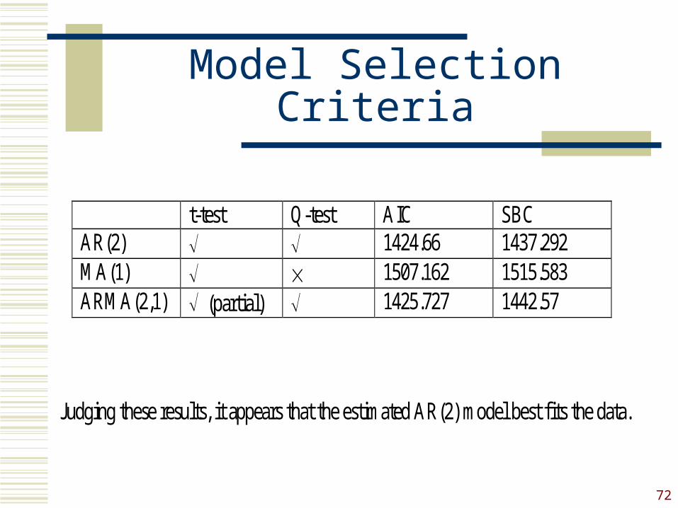
Model Selection Criteria
t-test Q-test AIC SBC AR(2) 1424.66 1437.292 MA(1) 1507.162 1515.583 ARMA(2,1) (partial) 1425.727 1442.57
Judging these results, it appears that the estimated AR(2) model best fits the data.

73
Step Four: Forecasting

74
Forecasting
The h-period ahead forecast based on an ARMA(p,q) model is given by
where elements on the r.h.s. of the equation may be replaced by their estimates when the actual values are not available.
qhtqhthtphtphtht eeeyyy ˆ.....ˆˆ.....ˆˆˆ 1111

75
Forecasting
For the AR(2) model,
For the MA(1) model,
0418.54339893.249115.04410.435039.068115.4ˆ
4410.42253477.249115.04339893.235039.068115.4ˆ
2498
1498
y
y
10209.4)0(48367.0010209.4ˆ
7508.3)7263.0(48367.0010209.4ˆ
2498
1498
y
y