1 Neuro-Dynamic Programming José A. Ramírez , Yan Liao Advanced Decision Processes ECECS 841,...
89
1 Neuro-Dynamic Programming José A. Ramírez , Yan Liao Advanced Decision Processes ECECS 841, Spring 2003 University of Cincinnati
-
date post
21-Dec-2015 -
Category
Documents
-
view
217 -
download
0
Transcript of 1 Neuro-Dynamic Programming José A. Ramírez , Yan Liao Advanced Decision Processes ECECS 841,...

1
Neuro-Dynamic Programming
José A. Ramírez , Yan LiaoAdvanced Decision Processes
ECECS 841, Spring 2003University of Cincinnati

Neuro-Dynamic Programming - ECECS 841- Advanced Decision Processes - J.Ramirez & Y. Liao
2
Outline1. Neuro-Dynamic Programming (NDP): motivation.
2. Introduction to Infinite Horizon Problems Minimization of Total Cost, Discounted Problems, Finite-State Systems,
Value Iteration and Error Bounds, Policy Iteration,
The Role of Contraction Mappings.
3. Stochastic Control Overview: State Equation (system model), Value Function, Stationary policies and value function, Introductory example: Tetris (game).
Neuro-Dynamic Programming - ECECS 841- Advanced Decision Processes - J.Ramirez & Y. Liao
3
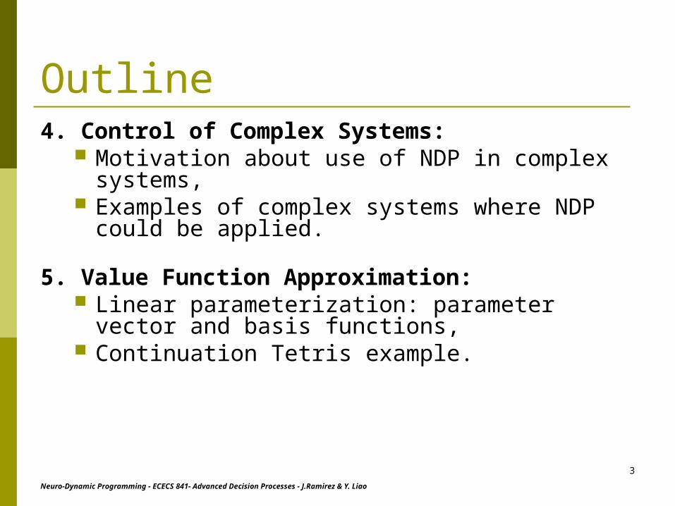
Outline4. Control of Complex Systems:
Motivation about use of NDP in complex systems, Examples of complex systems where NDP could be
applied.
5. Value Function Approximation: Linear parameterization: parameter vector and basis
functions, Continuation Tetris example.

Neuro-Dynamic Programming - ECECS 841- Advanced Decision Processes - J.Ramirez & Y. Liao
4
Outline6. Temporal-Difference Learning (TD()):
Introduction: Autonomous systems, general TD() algorithm, Controlled Systems, TD() for more general systems:
Approximate policy iteration, Controlled TD, Q-functions, and approximating the Q-function (Q-
learning), Comments about relationship with Approximate Value
Iteration.7. Actors and Critics:
Averaged Rewards, Independent actors, Using critic Feedback.
Neuro-Dynamic Programming - ECECS 841- Advanced Decision Processes - J.Ramirez & Y. Liao
5
1. Neuro-Dynamic Programming (NDP): motivation
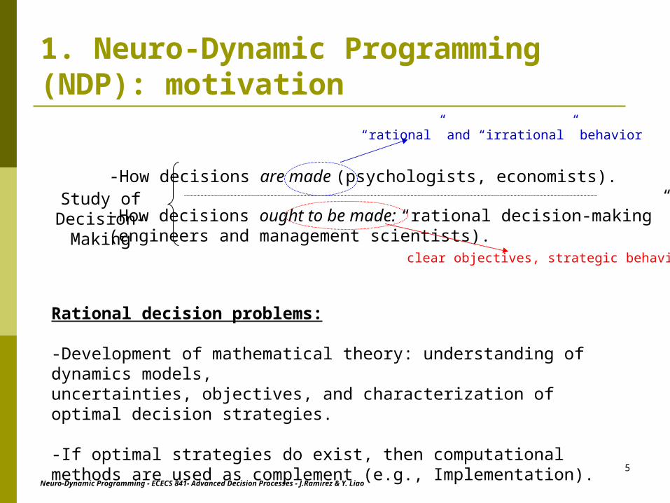
Study ofDecision-Making
-How decisions are made (psychologists, economists).
-How decisions ought to be made: “rational decision-making” (engineers and management scientists).
“rational” and “irrational” behavior
clear objectives, strategic behavior.
Rational decision problems:
-Development of mathematical theory: understanding of dynamics models,uncertainties, objectives, and characterization of optimal decision strategies.
-If optimal strategies do exist, then computational methods are used as complement (e.g., Implementation).

Neuro-Dynamic Programming - ECECS 841- Advanced Decision Processes - J.Ramirez & Y. Liao
6
1. Neuro-Dynamic Programming (NDP): motivation
-In contrast to rational decision-making, there is no clear-cut mathematical theory about decisions made by participants of natural systems (speculative theories, refining ideas by experimentation).
-One approach: hypothesis that behavior is in some sense rational, then ideas from study of rational decision-making are used to characterize such behavior, e.g., utility and equilibrium theory in financial economics.
-Also, study of animal behavior is subject of interest: evolutionary theory and its popular precept “survival of the fittest” –support the possibility that behavior to some extent concurs with that rational agent.
-Contributions from study of natural systems to science of rational decision-making:
-Computational complexity of decision problems and lack of systematic approaches for dealing with it.
Neuro-Dynamic Programming - ECECS 841- Advanced Decision Processes - J.Ramirez & Y. Liao
7
1. Neuro-Dynamic Programming (NDP): motivation
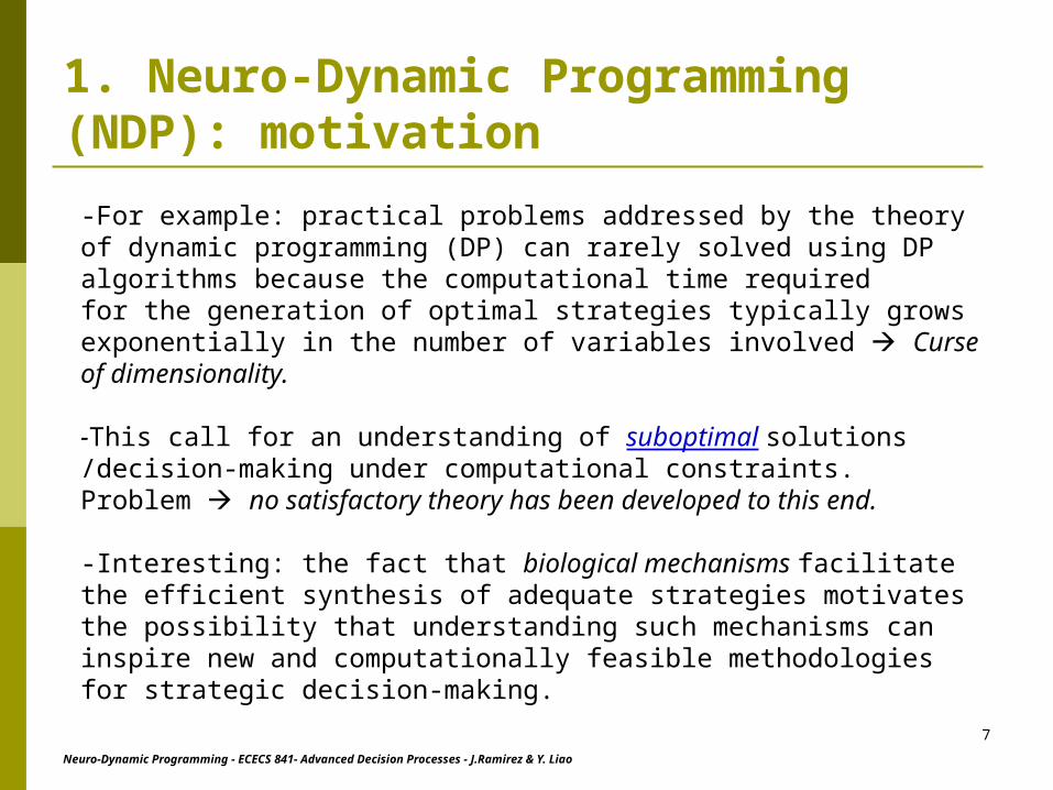
-For example: practical problems addressed by the theory of dynamic programming (DP) can rarely solved using DP algorithms because the computational time required
for the generation of optimal strategies typically grows exponentially in the number of variables involved Curse of dimensionality.
-This call for an understanding of suboptimal solutions /decision-making under computational constraints. Problem no satisfactory theory has been developed to this end.
-Interesting: the fact that biological mechanisms facilitate the efficient synthesis of adequate strategies motivates the possibility that understanding such mechanisms can inspire new and computationally feasible methodologies for strategic decision-making.

Neuro-Dynamic Programming - ECECS 841- Advanced Decision Processes - J.Ramirez & Y. Liao
8
1. Neuro-Dynamic Programming (NDP): motivation
-Reinforcement Learning (RL): over two decades, RL algorithms –originally conceived as descriptive models for phenomena observed in animal behavior- have grown out in the field of artificial intelligence and been applied to solving complex sequential decision problems.
-Success of RL in solving large-scale problems has generated special interest among operations researchers and control theorists research devoted to understand those methods and their potential.
-Developments from the operations research and control theorists: focused in normative view, acknowledge of relative disconnect from descriptive models of animal behavior, some operations researchers and control theorists have come to refer this area of research as Neuro-Dynamic Programming (NDP) instead of RL.

Neuro-Dynamic Programming - ECECS 841- Advanced Decision Processes - J.Ramirez & Y. Liao
9
1. Neuro-Dynamic Programming (NDP): motivation
-During these lectures we will present a sample of the recent developments and open issues of research in NDP.
-Specifically, we will be focused in two algorithmic ideas of greatest use in NDP, and for which there has been significant theoretical progress in recent years:
-Temporal-Difference learning-Actor-Critic Methods.
-First, we begin providing some background and perspective on the methodology and problems may address.
Comments about references

Neuro-Dynamic Programming - ECECS 841- Advanced Decision Processes - J.Ramirez & Y. Liao
10
2. Introduction to Infinite Horizon ProblemsMaterial taken from “Dynamic Programming and Optimal Control”, vol. I, II; and “Neuro-Dynamic Programming” by Dimitri P. Berstsektas and John Tsitsiklis.
The Dynamic Programming Problems with infinite horizon are characterized by the following aspects:a) The number of stages is infinite*.b) The system is stationary the system equation, the cost per stage, and the random disturbance statistics do not change from one stage to the next.
Why Infinite Horizon Problems?: -They are interesting because their analysis is elegant and insightful.-Implementation of optimal policies is often simple. Optimal policies
are typically stationary, e.g., optimal rule used to choose controls does not change from stage to stage.-NDP! complex systems.
*This assumption is never satisfied in practice, but is a reasonable approximation for problems with a finite but very large number of stages.

Neuro-Dynamic Programming - ECECS 841- Advanced Decision Processes - J.Ramirez & Y. Liao
11
2. Introduction to Infinite Horizon Problems-They require more sophisticated analysis than the finite horizon problems. It is needed to analyze limiting behavior as the horizon tends to infinity.
-We consider four principal classes of infinite horizon problems. The first two classes try to minimize J (x0), the total cost over an infinite number of stages:
i) Stochastic shortest path problems: in this case = 1 and assume that there is an additional state 0, which is a cost-free termination state; once the system reach the termination state it remains there at not additional cost. objective: reach the termination state with the minimal cost.
ii) Discounted problems with bounded cost per stage: here < 1, and the absolute one-stage cost |g(x,u,w)| is bounded from above by some constant M. Thus, J(x0) is well defined because it is the infinite sum of a sequence of numbers that are bounded in absolute value by the decreasing geometric progression Mk.
factor.discount 1
000
10
:,xx)w),x(,x(gElim)x(JN
kkkkk
k
wkN,...,k

Neuro-Dynamic Programming - ECECS 841- Advanced Decision Processes - J.Ramirez & Y. Liao
12
2. Introduction to Infinite Horizon Problemsiii) Discounted problems with unbounded cost per stage: here the discount factor
may or may not be less than 1, and the cost per stage is unbounded. this problem is difficult to analyze because of the possibility of infinite cost for some policies (more details in chap.3, Dynamic Programming,vol. II, by Bertsekas).
iv) Average cost problems: in some problems we have J(x0) =, for every policy and initial state i, then in many problems the average cost per stage, given by
where JN(i) is the N-stage cost-to-go of policy starting at state x0, is well defined
as a limit and is finite.
,1 1
0
))w),x(,x(g(JN
limN
kkkkkN
N

Neuro-Dynamic Programming - ECECS 841- Advanced Decision Processes - J.Ramirez & Y. Liao
13
2. Introduction to Infinite Horizon ProblemsA Preview of Infinite Horizon Results:
Let J* the optimal cost-to-go function of the infinite horizon problem, and consider the case = 1, with JN(x) as the optimal cost of the problem involving N stages, initial state x, cost per stage g(x,u,w), and zero terminal cost. Thus, the N-stage cost can be computed after N iterations of the DP algorithm*:
Thus, we can speculate the following:
i) The optimal infinite horizon cost is the limit of the corresponding N-stage optimal costs as N ∞ :
.)x(J,))w,,x(f(J)w,,x(gEmin)x(J k)x(Uu
k 0 01
.x)x(Jlim)x(J NN
*
*Note that the time indexing has been reversed from the original DP algorithm, thus the optimal finite horizon cost functions can be computed with a singleDP recursion (more details in chap.1, “Dynamic Programming”, vol. II, by D.P. Bertsekas.

Neuro-Dynamic Programming - ECECS 841- Advanced Decision Processes - J.Ramirez & Y. Liao
14
2. Introduction to Infinite Horizon Problemsii) The following limiting form of the DP algorithm should hold for all states:
this is not an algorithm, but a system of equations (one equation per state), which has as solution the costs-to-go for all states. It is also viewed as a functional equation for the cost-to-go function J* , and it is called Bellman’s equation.
iii) If (x) attains the minimum in the right-hand side of the Bellman’s equation for each x, then the policy ={, , …} should be optimal. This is true for most infinite horizon problems of interest. stationary policies.
Most of the analysis of infinite horizon problems are focused around the above three issues and efficient methods to compute J* and optimal policies.
))w,,x(f(J)w,,x(gEmin)x(J *
)x(Uu
*

Neuro-Dynamic Programming - ECECS 841- Advanced Decision Processes - J.Ramirez & Y. Liao
15
2. Introduction to Infinite Horizon ProblemsStationary Policy:A stationary policy is an admissible policy ={, , …} with a corresponding cost function J (x). is optimal if J(x)=J*(x) for all states x.
Some Shorthand Notation:The use of single recursions in the DP algorithm to compute optimal costs over a finite horizon, motivates the introduction of two mappings that play an important theoretical role and give us a convenient shorthand notation for expressions that are Complicated to write.
For any function J:S, where S is the states space, we consider the function obtained by applying the DP mapping J as follows:
T can be viewed as a mapping that transforms J on S into the function TJ on S. TJ represent the optimal cost function for the one-stage problem that has stage cost g and terminal cost J.
.Sx,))w,,x(f(J)w,,x(gEmin)x)(TJ( *
)x(Uu

Neuro-Dynamic Programming - ECECS 841- Advanced Decision Processes - J.Ramirez & Y. Liao
16
2. Introduction to Infinite Horizon ProblemsSimilarly, for any control function : S C, where C is the space of controls, we have:
Also, we denote the composition Tk of the mapping T with itself k times
Then, for k=0 we have
.Sx,))w),x(,x(f(J)w),x(,x(gEmin)x)(JT( *
)x(Uu
.Sx),x))(JT(T()x)(JT( kk 1
.Sx),x))(JT(T()x)(JT( kk 1

Neuro-Dynamic Programming - ECECS 841- Advanced Decision Processes - J.Ramirez & Y. Liao
17
2. Introduction to Infinite Horizon ProblemsSome Basic Properties
Monotonicity Lemma: For any functions J:S and J’:S, such that
and for any function :SC with (x) U(x), for all x S, we have
,Sx),x('J)x(J
,...,k,Sx),x)('JT()x)(JT(
,...,,k,Sx),x)('JT()x)(JT(kk
kk
10
10

Neuro-Dynamic Programming - ECECS 841- Advanced Decision Processes - J.Ramirez & Y. Liao
18
2. Introduction to Infinite Horizon ProblemsThe Role of Contraction Mappings (Dynamic Programming, vol. II, Bertsekas)
Definition 1.4.1: A mapping H: B(S) B(S) is said to be a contraction mapping if there exists a scalar <1 such that
Where || ∙ || is the norm
It is said to be an m-stage contraction mapping if there exists a positive integer m and
some < 1 such that
where Hm denotes the composition of H with itself m times.
Note: B(S) is the set of all bounded real-valued functions on S. Every function J:S .
),S(B'J,J,'JJ'HJHJ
.)x(JmaxJXx
),S(B'J,J,'JJ'JHJH mm

Neuro-Dynamic Programming - ECECS 841- Advanced Decision Processes - J.Ramirez & Y. Liao
19
2. Introduction to Infinite Horizon ProblemsThe Role of Contraction Mappings (Dynamic Programming, vol. II, Bertsekas)
Proposition 1.4.1: (Contraction Mapping Fixed-Point Theorem)If H: B(S) B(S) is a contraction mapping or an m-stage contraction mapping, then there exists a unique fixed point of H; i.e., there exists a unique function J* B(S) such that
Furthermore, if J is any function in B(S) and Hk is the composition of H with itself k times, then
.JHJ **
0.
*k
kJJHlim

Neuro-Dynamic Programming - ECECS 841- Advanced Decision Processes - J.Ramirez & Y. Liao
20
3. Stochastic Control Overview
State Equation: Let’s consider a discrete-time dynamic system, that at each time t, takes on a state xt and evolves according to:
),w,a,x(fx tttt 1
where wt is a disturbance (iid) and at is a control decision. We restrict attention to finite state, disturbances, and control spaces, denoted by , W, and , respectively.
Value Function: Let r : x associates a reward r( xt , at ) with a decision at, made at state xt. Let a stationary policy with : . For each policy we define a value function v( ∙ , ) : :
.xx))x(,x(rE),x(vt
ttt
00
factor.discount
1 0,
:

Neuro-Dynamic Programming - ECECS 841- Advanced Decision Processes - J.Ramirez & Y. Liao
21
3. Stochastic Control Overview
Optimal Value Function: we define the optimal value function V as follows:
From dynamic programming, we have that any stationary policy * given by
).,(max)(
xvxV
,)),,((),(maxarg)(* waxfVaxrEx wAa
is optimal in the sense that
),x(v)x(V *

Neuro-Dynamic Programming - ECECS 841- Advanced Decision Processes - J.Ramirez & Y. Liao
22
3. Stochastic Control Overview
Example 1: TetrisThe video arcade game of Tetris can be viewed as an instance of stochastic control. In particular, we can view the state xt as an encoding of the current “wall of bricks” and the shape of the current “falling piece.” The decision at identifies an orientation and horizontal position for placement of the falling piece onto the wall. Though the arcade game employs a more complicated scoring system, consider for simplicity a reward r(xt, at) equal to the number of rows eliminated by placing the piece in the position described by a t. Then, a stationary policy that maximizes the value
,))(,(),(0
0
ttt
t xxxxrExv
essentially optimizes a combination of present and future row elimination, with decreasing emphasis placed on rows to be eliminated at times farther into the future.

Neuro-Dynamic Programming - ECECS 841- Advanced Decision Processes - J.Ramirez & Y. Liao
23
3. Stochastic Control Overview
Example 1: Tetris, cont.Tetris was first programmed by Alexey Pajitnov, Dmitry Pavlovsky, and Vadim Gerasimov, computer engineers at the Computer Center of the Russian Academy of Sciences in 1985-86.
Standard shapes
h=20
w=10Number of states
states. 10248127
shapes ofnumber 2612010
.
:mm wh

Neuro-Dynamic Programming - ECECS 841- Advanced Decision Processes - J.Ramirez & Y. Liao
24
3. Stochastic Control Overview
Dynamic programming algorithms compute the optimal value function V. The result is stored in a “look-up” table with one entry V(x) per state x X. When is required, the value function is used to generate optimal decisions. For example, given a current state xt X , a decision at is selected according to
.)),,((),(maxarg waxfVaxrEa ttwAa
t

Neuro-Dynamic Programming - ECECS 841- Advanced Decision Processes - J.Ramirez & Y. Liao
25
4. Control of Complex Systems
The main objective is in the development of a methodology for the control of “complex systems”.
Two common characteristics of these type of systems are:
i-An intractable state space : intractable state spaces preclude the use of classical DP which compute and store one numerical value per state.
ii- Severe nonlinearities: methods of traditional linear control, which are applicable even in large state spaces, are ruled out by severe nonlinearities.
Let’s review some examples of complex systems, where NDP could be and has been applied.

Neuro-Dynamic Programming - ECECS 841- Advanced Decision Processes - J.Ramirez & Y. Liao
26
4. Control of Complex Systemsa) Call Admission and RoutingWith rising demand in telecommunication network resources, effective management is as important as ever. Admission (deciding which calls to accept/reject) and routing (allocating links in the network to particular calls) are examples of decisions that must be made at any point in time. The objective is to make the “best” use of limited network resources. In principle, such sequential decision problems can be addressed by dynamic programming. Unfortunately, the enormous state spaces involved render dynamic programming algorithms inapplicable, and heuristic control strategies are used in lieu.
b) Strategic Asset AllocationStrategic asset allocation is the problem of distributing an investor’s wealth among assets in the market in order to take on a combination of risk and expected return that best suits the investor’s preferences. In general, the optimal strategy involves dynamic rebalancing of wealth among assets over time. If each asset offers a fixed rate of risk and return, and some additional simplifying assumptions are made, the only state variable is wealth, and the problem can be solved efficiently by dynamic programming algorithms. There are even closed form solutions in cases involving certain types of investor preferences. However, in the more realistic setting involving risks and returns that fluctuate with economic conditions, economic indicators must be taken into account as state variables, and this quickly leads to an intractable state space. The design of effective strategies in such situations constitutes an important challenge in the growing field of financial engineering.

Neuro-Dynamic Programming - ECECS 841- Advanced Decision Processes - J.Ramirez & Y. Liao
27
4. Control of Complex Systemsc) Supply–Chain ManagementWith today’s tight vertical integration, increased production complexity, and diversification, the inventory flow within and among corporations can be viewed as a complex network – called a supply chain – consisting of storage, production, and distribution sites. In a supply chain, raw materials and parts from external vendors are processed through several stages to produce finished goods. Finished goods arethen transported to distributors, then to wholesalers, and finally retailers, before reaching customers. The goal in supply–chain management is to achieve a particular level of product availability while minimizing costs. The solution is a policy that decides how much to order or produce at various sites given the present state of the company and the operating environment.
d) Emissions ReductionsThe threat of global warming that may result from accumulation of carbon dioxide and other “greenhouse gasses” poses a serious dilemma. In particular, cuts in emission levels bear a detrimental short–term impacton economic growth. At the same time, a depleting environment can severely hurt the economy – especially the agricultural sector – in the longer term. To complicate the matter further, scientific evidence on the relationship between emission levels and global warming is inconclusive, leading to uncertainty about the benefits of various cuts. One systematic approach to considering these conflicting goals involves the formulation of a dynamic system model that describes our understanding of economic growth and environmental science. Given such a model, the design of environmental policy amountsto dynamic programming. Unfortunately, classical algorithms are inapplicable due to the size of the state space.
Neuro-Dynamic Programming - ECECS 841- Advanced Decision Processes - J.Ramirez & Y. Liao
28
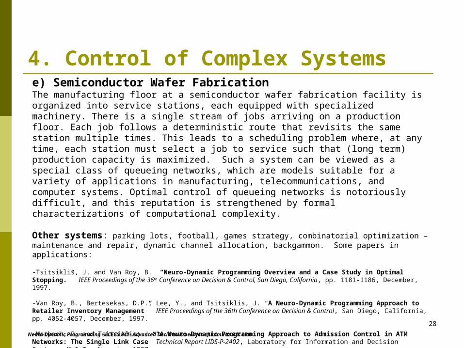
4. Control of Complex Systemse) Semiconductor Wafer FabricationThe manufacturing floor at a semiconductor wafer fabrication facility is organized into service stations, each equipped with specialized machinery. There is a single stream of jobs arriving on a production floor. Each job follows a deterministic route that revisits the same station multiple times. This leads to a scheduling problem where, at any time, each station must select a job to service such that (long term) production capacity is maximized. Such a system can be viewed as a special class of queueing networks, which are models suitable for a variety of applications in manufacturing, telecommunications, and computer systems. Optimal control of queueing networks is notoriously difficult, and this reputation is strengthened by formal characterizations of computational complexity.
Other systems: parking lots, football, games strategy, combinatorial optimization – maintenance and repair, dynamic channel allocation, backgammon. Some papers in applications:
-Tsitsiklis, J. and Van Roy, B. “Neuro-Dynamic Programming Overview and a Case Study in Optimal Stopping.” IEEE Proceedings of the 36th Conference on Decision & Control, San Diego, California, pp. 1181-1186, December, 1997.
-Van Roy, B., Bertesekas, D.P., Lee, Y., and Tsitsiklis, J. “A Neuro-Dynamic Programming Approach to Retailer Inventory Management” IEEE Proceedings of the 36th Conference on Decision & Control, San Diego, California, pp. 4052-4057, December, 1997.
-Marbach, P. and Tsitsiklis, J. “A Neuro-Dynamic Programming Approach to Admission Control in ATM Networks: The Single Link Case” Technical Report LIDS-P-2402, Laboratory for Information and Decision Systems, M.I.T., November 1997.
- Marbach, P, Mihatsch, O, and Tsitsiklis, J. “Call Admission Control and Routing in Integrated Services Networks Using Reinforcement Learning” IEEE Proceedings of the 37th Conference on Decision & Control, Tampa, Florida, pp. 563-568, December, 1998.
-Bertsekas, D.P., Homer, M.L., “Missile Defense and Interceptor Allocation by Neuro-Dynamic Programming” IEEE Transactions on Systems Man and Cybernetics, vol. 30, pp.101-110, 2000.

Neuro-Dynamic Programming - ECECS 841- Advanced Decision Processes - J.Ramirez & Y. Liao
29
4. Control of Complex Systems
-For the examples presented, state spaces are intractable as consequence of the “curse of dimensionality”, that is, state spaces grow exponentially in the number of state variables. difficult (if not impossible) to compute (store) one value per state as is required by classical DP.
-Additional shortcoming with classical DP: computations require use of transition probabilities. For many complex systems, such probabilities are not readily accessible. On the other hand, is often easier develop simulation models for the system and generate sample trajectories.
-Objective of NDP: overcoming curse of dimensionality through use of parameterized (value) function approximators and through use of output generated by simulators, rather than explicit transition probabilities.

Neuro-Dynamic Programming - ECECS 841- Advanced Decision Processes - J.Ramirez & Y. Liao
30
5. Value Function Approximation
-Intractability of state spaces value function approximation.
-Two important pre-conditions for the development of effective approximation:
i-Choose a parameterization*: that yields a good approximation
ii-Algorithms for computing appropriate parameter values.
*Note: the choice of a suitable parameterization requires some practical experience or theoretical analysis that provides rough information about the shape of the function to be approximated.
KXv :~
),(),(~ xVuxv Kuu vector,parameter :

Neuro-Dynamic Programming - ECECS 841- Advanced Decision Processes - J.Ramirez & Y. Liao
31
5. Value Function Approximation
Linear parameterization*
-General classes of parameterizations have been found used in NDP, to keep the exposition simple, let us focus on linear parameterizations, which take the form
,)()(),(~1
K
kk xkuuxv
where 1, …, K are “basis functions” mapping X to and u = (u(1), …, u(K))’ is a vector of scalar weights.
Similar to statistical regression, the basis functions 1, …, K are selected by a human based on intuition or analysis to the problem at hand.
Hint: one interpretation that is useful for the construction of basis functions involves viewing each function k as a “feature” – that is, a numerical value capturing a salient characteristic of the state that may be pertinent to effective decision making.

Neuro-Dynamic Programming - ECECS 841- Advanced Decision Processes - J.Ramirez & Y. Liao
32
5. Value Function Approximation
Example 2: Tetris, continuation.In our stochastic control formulation of Tetris, the state is an encoding of the current wall configuration and the current falling piece. There are clearly too many states for exact dynamic programming algorithms to be applicable. However, we may believe that most information relevant to game–playing decisions can be captured by a few intuitive features. In particular, one feature, say 1, may map states to the height of the wall. Another, say 2, could map states to a measure of “jaggedness” of the wall. A third might provide a scalar encoding of the type of the current falling piece (there are seven different shapes in the arcade game). Given a collection of such features, the next task is to select weights u(1), . . . , u(K) such that
for all states x. This approximation could then be used to generate a game–playing strategy.
),()()(1
xVxkuK
kk
Neuro-Dynamic Programming - ECECS 841- Advanced Decision Processes - J.Ramirez & Y. Liao
33
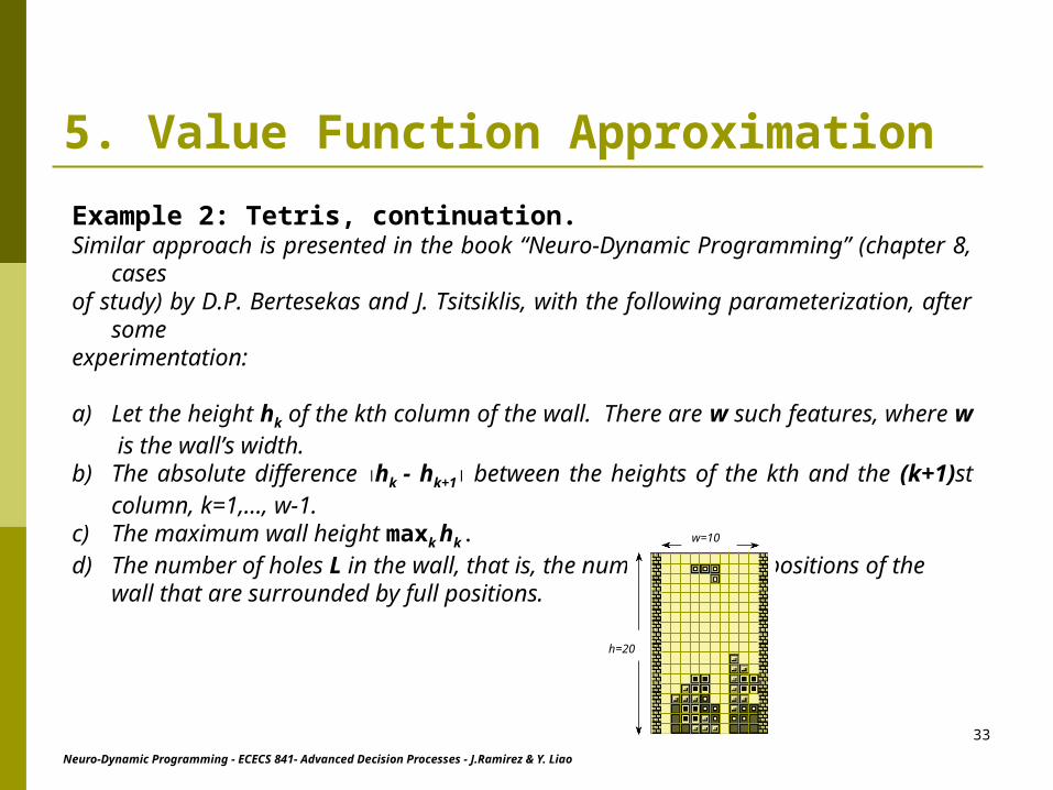
5. Value Function Approximation
Example 2: Tetris, continuation.Similar approach is presented in the book “Neuro-Dynamic Programming” (chapter 8, casesof study) by D.P. Bertesekas and J. Tsitsiklis, with the following parameterization, after someexperimentation:
a) Let the height hk of the kth column of the wall. There are w such features, where w is the wall’s width.
b) The absolute difference hk - hk+1 between the heights of the kth and the (k+1)st column, k=1,…, w-1.
c) The maximum wall height maxk hk.d) The number of holes L in the wall, that is, the number of empty positions of the wall that
are surrounded by full positions.
h=20
w=10

Neuro-Dynamic Programming - ECECS 841- Advanced Decision Processes - J.Ramirez & Y. Liao
34
5. Value Function Approximation
Example 2: Tetris, continuation.
Thus, there are 2w+1 features, which together with a constant offset, require 2w+2 weights in alinear architecture of the form
Using this parameterization, with w=10 (22 features), an strategy is generated by NDP thateliminates an average of 3554 rows per game, reflecting performance comparable of an expertplayer.
.)12(max)2()()()0(),(~1
11
1
Lwuhwuhhwkuhkuuuxv kk
w
kkk
w
kk
offset

Neuro-Dynamic Programming - ECECS 841- Advanced Decision Processes - J.Ramirez & Y. Liao
35
6. Temporal-Difference LearningIntroduction to Temporal-Difference Learning
Material from:Richard Sutton, “Learning to Predict by Methods of Temporal Differences”, MachineLearning, 3: 9-44, 1988. this paper provide the first formal results in the theory of temporal-difference (TD) methods.
- “Learning to predict”:-Use of past experience (historical information) with a incompletely know
system to predict its future behavior.-”Learning to predict“ is one of the most basic and prevalent kinds of learning.-In prediction learning training examples can be taken directly from the
temporal -sequence of ordinary sensory input; no special supervisor or teacher is required.
-Conventional prediction-learning methods (Widrow-Hoff, LMS, Delta Rule, Backpropagation):
-Driven by error between predicted and actual outcomes.

Neuro-Dynamic Programming - ECECS 841- Advanced Decision Processes - J.Ramirez & Y. Liao
36
6. Temporal-Difference Learning
-TD methods:• Driven by error or difference between temporally successive predictions.
learning occurs whenever there is a change in prediction over time.
-Advantages of TD methods over conventional methods:• They are more incremental, and therefore more easier to compute.
• They tend to make more efficient use of their experience: they converge faster and produce better predictions.
-TD Approach:• Predictions are based on numerical features combined using adjustable
parameters or “weights”. similar to connectionist models (Neural Networks)

Neuro-Dynamic Programming - ECECS 841- Advanced Decision Processes - J.Ramirez & Y. Liao
37
6. Temporal-Difference Learning
-TD and supervised-learning approaches to prediction:• Historically, the most important learning paradigm has been supervised learning:
learner is asked to associate pairs of items (input,output).
• Supervised learning has been used in patter classification, concept acquisition, learning from examples, system identification, and associative memory.
AInput Real Output
Input
Estimated OutputA
+
-
Error LearningAlgorithm
Adjust estimator parameters

Neuro-Dynamic Programming - ECECS 841- Advanced Decision Processes - J.Ramirez & Y. Liao
38
6. Temporal-Difference Learning
-Single-step and multi-step prediction problems:• Single-step: all information about the correctness of each prediction is revealed at
once. supervised learning methods.
• Multi-step: correctness is not revealed until more than one step after the prediction is made, but partial information relevant to its correctness is revealed at each step. TD learning methods.
-Computational issues:• Sutton introduce a particular TD procedure by formally relating it to a classical
supervised-learning procedure, the Widrow-Hoff rule (also known as “delta rule’, the ADALINE –Adaptive Linear Element, and the Least Mean Squares –LMS- filter).
• We consider multi-step prediction problems in which experience comes in observation-outcome sequences of the form x1, x2, x3, …, xm, z, where each xt is a vector of observations available at time t in the sequence, and z is the outcome of the sequence. Also, xt n and z .

Neuro-Dynamic Programming - ECECS 841- Advanced Decision Processes - J.Ramirez & Y. Liao
39
6. Temporal-Difference Learning-Computational issues (cont.):
• For each observation-outcome, the learner produces a corresponding sequence of predictions P1, P2, P3, …, Pm, each of which is an estimate of z.
• Predictions Pt are based on a vector of modifiable parameters w. Pt(xt ,w)
• All learning procedures are expressed as rules for updating w. For each observation, an increment to w, denoted wt , is determined. After a complete sequence has been processed, w is changed by (the sum of) all the sequences increments:
• The supervised-learning approach treats each sequence of observations and its outcome as a sequence of observation-outcome pairs: (x1 , z) , (x2 , z), …, (xm , z). In this case increments due to time t depends on the error between Pt and z, and on how to change w will affect Pt .
m
ttwww
1

Neuro-Dynamic Programming - ECECS 841- Advanced Decision Processes - J.Ramirez & Y. Liao
40
6. Temporal-Difference Learning-Computational issues (cont.):
• Then, a prototypical supervised-learning update procedure is
where is a positive parameter affecting the rate of learning, and the gradient wPt , isthe vector of partial derivatives of Pt with respect to each component of w.
• Special case: consider Pt a linear function of xt and w, that is Pt = wTxt = i w(i) xt(i), where w(i) and xt(i) are ith component of w and xt. wPt = xt. Thus,
which correspond to the Widrow-Hoff rule.
• This equation depend critically on z, and thus cannot be determined until the end of the sequence when z becomes known. All observations and predictions made during a sequence must be remembered until its end: wt cannot be computed incrementally.
,P)Pz(w twtt
,x)xwz(w ttT
t
Neuro-Dynamic Programming - ECECS 841- Advanced Decision Processes - J.Ramirez & Y. Liao
41
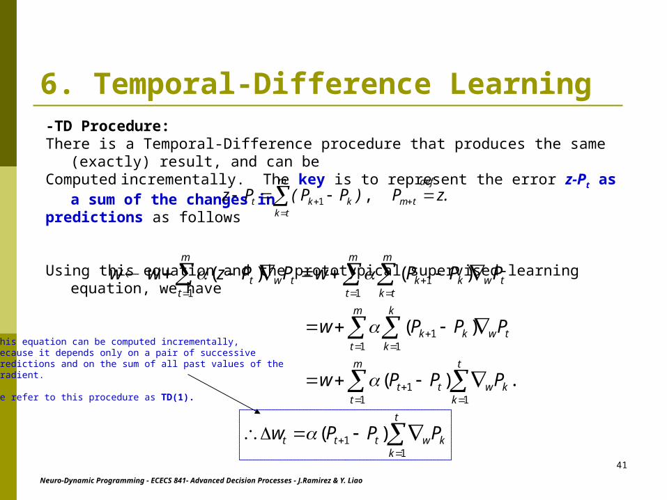
6. Temporal-Difference Learning-TD Procedure:There is a Temporal-Difference procedure that produces the same (exactly) result, and can beComputed incrementally. The key is to represent the error z-Pt as a sum of the changes in predictions as follows
Using this equation and the prototypical supervised-learning equation, we have
.zP)PP(Pzdef
tm
m
tkkkt
, 1
t
kkwttt
m
t
t
kkwtt
tw
m
t
k
kkk
tw
m
t
m
tkkktw
m
tt
PPPw
PPPw
PPPw
PPPwPPzww
11
1 11
1 11
11
1
)(
.)(
)(
)()(
This equation can be computed incrementally,because it depends only on a pair of successivepredictions and on the sum of all past values of thegradient.
We refer to this procedure as TD(1).

Neuro-Dynamic Programming - ECECS 841- Advanced Decision Processes - J.Ramirez & Y. Liao
42
6. Temporal-Difference LearningThe TD() family of learning procedures:
• The “hallmark” of temporal-difference methods is their sensitivity to changes in successive predictions rather than overall error between predictions and the final outcome.
• In response to an increase (decrease) in prediction from Pt to Pt+1 , an increment wt is
determined that increases (decreases) the predictions for some or all of the preceding observations vectors x1, …,xt.
• TD(1) is a special case where all the predictions are altered to an equal extent.
• Now, consider the case where greater alterations are made to more recent predictions. We consider an exponential weighting with recency, in which alterations to the predictions of observation vectors occurring k steps in the past are weighted according to k for 0 1:
t
kkw
ktttt PPPw
11 )( 1
0
t-k
=1, TD(1)
0 < < 1
=0TD(0)
t-k
k increases

Neuro-Dynamic Programming - ECECS 841- Advanced Decision Processes - J.Ramirez & Y. Liao
43
6. Temporal-Difference LearningThe TD() family of learning procedures:
• For =0 we have the TD(0) procedure:
• For =1 we have the TD(1) procedure, that is equivalent to the Widrow-Hoff rule, except that TD(1) is incremental:
• Alterations of past predictions can be weighted in ways other than the exponential form given previously, let
tttttwtttttwt
t
kkw
kttw
t
kkw
kttw
t
kkw
kttw
tt
t
kkw
ktt
t
kkw
ktt
ePPePPPwePe
PP
PPPP
ttkPe
Pe
)())((
.1,,...,1
11111
11
1
11
1
11
)1(1
1
1
11
1
Also referred in literature as eligibility vectors.
t
kkwttt PPPw
11 )(
twttt P)PP(w 1

Neuro-Dynamic Programming - ECECS 841- Advanced Decision Processes - J.Ramirez & Y. Liao
44
6. Temporal-Difference Learning(Material taken from Neuro-Dynamic Programming, Chapter 5)
Monte Carlo Simulation: brief overview
• Suppose v is a random variable with unknown mean m that we want to estimate. • Using Monte Carlo simulation to estimate m: generate a number of samples v1, v2, …, vN,
and then estimate m by forming the sample mean
Also, we can compute the sample mean recursively
with M1 = v1 .
.1
1
N
kkN v
NM
),(1
111 NNNN Mv
NMM

Neuro-Dynamic Programming - ECECS 841- Advanced Decision Processes - J.Ramirez & Y. Liao
45
6. Temporal-Difference LearningMonte Carlo simulation: case of iid samples
Suppose N samples v1, v2, …, vN , independent and identically distributed, with mean m, andvariance 2. Then we have
where MN is said to be an unbiased estimator of m. Also, its variance is given by
As N the variance of MN converge to zero MN converges to m.
Also, the strong law of large numbers provides an additional property: the sequence MN converges to m with probability one. The estimator is consistent.
,}{1
}{1
mvEN
MEN
kkN
,)(1
)(2
12 N
vVarN
MVarN
kkN

Neuro-Dynamic Programming - ECECS 841- Advanced Decision Processes - J.Ramirez & Y. Liao
46
6. Temporal-Difference LearningPolicy Evaluation by Monte Carlo simulation
-Consider the stochastic shortest path problem, with state space {0, 1, 2, …, n} with 0 as an absorbing state and cost-free. Let the cost-to-go from i to j g( i , j ) (given the control action μ(i) , pij(μ(i))). Suppose that we have a fixed stationary policy μ (proper) and we want to
calculate, using simulation, the corresponding cost-to-go vector
J μ’ = ( J μ (1) J μ (2) . . . J μ (n) ).
Approach: generate, starting from each i, many samples states trajectories and average the corresponding costs to obtain an approximation to J μ(i). Instead of do this for each state i, lets use each trajectory to obtain cost samples for all states visited by the trajectory, and consider the cost of the trajectory portion that starts at each intermediate state.

Neuro-Dynamic Programming - ECECS 841- Advanced Decision Processes - J.Ramirez & Y. Liao
47
6. Temporal-Difference LearningPolicy Evaluation by Monte Carlo simulation
Suppose that a number of simulation runs are performed, each ending at the termination state 0. Consider the m-th time a given state i0 is encountered, and let (i0 , i1 ,…, iN) be the remainder of the corresponding trajectory, where iN = 0.
Then, let c( i0 , m ) the cumulative cost up to reaching state 0, then
Some assumptions: different simulated trajectories are statistically independent, and each trajectory is generated according to the Markov process determined by the policy μ. Then we have,
).,(...),(),( 1100 NN iigiigmic
)}.m,i(c{E)i(J

Neuro-Dynamic Programming - ECECS 841- Advanced Decision Processes - J.Ramirez & Y. Liao
48
6. Temporal-Difference LearningPolicy Evaluation by Monte Carlo simulation
The estimation of Jμ(i) is obtained by forming the sample mean
subsequent to the Kth encounter with state i. The sample mean can be expressed in iterative form:
where
starting with J(i)=0.
,...,2,1 )),(),(()(:)( miJmiciJiJ m
,...,2,1 ,1
mmm
,),(1
)(1
K
m
micK
iJ

Neuro-Dynamic Programming - ECECS 841- Advanced Decision Processes - J.Ramirez & Y. Liao
49
6. Temporal-Difference LearningPolicy Evaluation by Monte Carlo simulation
Consider the trajectory (i0, i1, …, iN), and let k an integer, such as 1 k N. The trajectory contains the subtrajectory (ik, ik+1,…, iN). sample trajectory with initial state ik that can be used to update J(ik) using the iterative equation previously presented.
Algorithm*:Run a simulation and generate the state trajectory (i0, i1, …,iN), update the estimates J(ik) for each k=0, 1, …, N-1, the formula
The step size γ(ik) can change from one iteration to iteration.
*Additional details Neuro-Dynamic Programming by Bertsekas and Tsitsiklis, chapter 5.
)),(),(...),(),()(()(:)( 1211 kNNkkkkkkk iJiigiigiigiiJiJ

Neuro-Dynamic Programming - ECECS 841- Advanced Decision Processes - J.Ramirez & Y. Liao
50
6. Temporal-Difference LearningMonte Carlo simulation using Temporal Differences
Here we consider the implementation of the Monte Carlo policy evaluation algorithm that incrementally updates the cost-to-go estimates J(i).
First, assume that for any trajectory i0, i1, …, iN , with iN = 0, and ik =0 for k > N,g( ik, ik+1) =0 for k N, and J(0)=0. Also, the policy under consideration is proper.
Lets rewrite the previous formula in the following form:
Note that we use the property J(iN)=0.
))).()(),((
))()(),((
)()(),((()(:)(
11
1221
11
NNNN
kkkk
kkkkkk
iJiJiig
iJiJiig
iJiJiigiJiJ

Neuro-Dynamic Programming - ECECS 841- Advanced Decision Processes - J.Ramirez & Y. Liao
51
6. Temporal-Difference LearningMonte Carlo simulation using Temporal Differences
Equivalently, we can rewrite the previous equation as follows:
where
are called temporal differences (TD). The TD represents the difference between the estimate
of the cost-to-go based on the simulated outcome in the current stage, and the current estimate J(ik).
),...()(:)( 11 Nkkkk dddiJiJ
),i(J)i(J)i,i(gd kkkkk 11
),(),( 11 kkk iJiig

Neuro-Dynamic Programming - ECECS 841- Advanced Decision Processes - J.Ramirez & Y. Liao
52
6. Temporal-Difference LearningMonte Carlo simulation using Temporal Differences
Advantage: The estimations can be computed incrementally, e.g., for the l-th temporal difference dl (once that it becomes available) we have
as soon as dl is available.
The temporal difference dl appears in the update formula for J(ik) for every k l, then,
as soon as transition il+1 has been simulated.
,N,...,kld)i(J)i(J lkk 1 , :
,l,...,k)),i(J)i(J)i,i(g)i(J
d)i(J)i(J
llllk
lkk
0 (
:
11

Neuro-Dynamic Programming - ECECS 841- Advanced Decision Processes - J.Ramirez & Y. Liao
53
Monte Carlo simulation using Temporal Differences: TD()
Here we introduce the TD() algorithm as a stochastic approximation method for solving a suitably reformulated Bellman equation.
The Monte Carlo evaluation algorithm can be viewed as a Robbins-Monro stochastic approximation (more details chapter 4. Neuro-Dynamic Programming) method for solving the equations
for unknowns J(ik), as ik ranges over the states in the state space. Other algorithms can be
generated in similar form, e.g., starting from other systems equation involving J and then replacing expectations by single estimates. For example, from Bellman’s equation
6. Temporal-Difference Learning
,)i,i(gE)i(Jm
mkmkk
01
)},i(J)i,i(g{E)i(J kkkk 11

Neuro-Dynamic Programming - ECECS 841- Advanced Decision Processes - J.Ramirez & Y. Liao
54
Monte Carlo simulation using Temporal Differences: TD()
the stochastic approximation method takes the form
which is updated each time that state ik is visited.
Lets take now a fixed value l, nonnegative and integer, and taking into consideration the cost for the first l+1 transitions, then the stochastic algorithm could be based on the (l+1)-step Bellman equation
Without any special knowledge to select one value of l over another, we consider forming a weighted average of all possible multistep Bellman equations. Specifically, we fix some < 1, and multiply by (1- ) l and sum over all nonnegative l.
6. Temporal-Difference Learning
,)i(J)i,i(gE)i(Jl
mlkmkmkk
0
11
)),i(J)i(J)i,i(g()i(J)i(J kkkkkk 11:
Neuro-Dynamic Programming - ECECS 841- Advanced Decision Processes - J.Ramirez & Y. Liao
55
Monte Carlo simulation using Temporal Differences: TD()
Then, we have
Interchanging the order of the two summations, and using the fact that we have
6. Temporal-Difference Learning
.)i(J)i,i(gE)()i(Jl
l
mlkmkmk
lk
0 0111
0
1l
ml .)(
)i(J)i(J)i(J)i,i(gE
))(i(J)i,i(g)(E)i(J
km
mkmkmkmkm
ml l
lllk
l
mmkmkk
011
0
11
01
1

Neuro-Dynamic Programming - ECECS 841- Advanced Decision Processes - J.Ramirez & Y. Liao
56
Monte Carlo simulation using Temporal Differences: TD()
The previous equation can be expressed in terms of the temporal differences as follows
where
are the temporal differences, and E{dm}=0 for all m (Bellman’s equation).
The Robbins-Monro stochastic approximation method, equivalent to the previous equation, is
where γ is a stepsize parameter (can change from iteration to iteration). The above equation provide us with a family of algorithms, one for each choice of , and it is known as TD(). Note that for =1 we have the Monte Carlo policy evaluation method, also called TD(1).
6. Temporal-Difference Learning
),i(JdE)i(J kkm
mkm
k
),i(J)i(J)i,i(gd mmmmm 11
,d)i(J:)i(Jkm
mkm
kk

Neuro-Dynamic Programming - ECECS 841- Advanced Decision Processes - J.Ramirez & Y. Liao
57
Monte Carlo simulation using Temporal Differences: TD()
Also, for =0, we have another limiting case, and using the convention 00=1, then the TD(0) method is presented as follows
This equation coincides with the one-step Bellman’s equation previously presented.
Off-line and On-line variants
When all of the updates are carried out simultaneously, after the entire trajectory has been simulated, then we have the off-line version of TD(). In alternative form, when the updates are evaluated one term at a time, we have the on-line version of TD().
6. Temporal-Difference Learning
)).i(J)i(J)i,i(g()i(J:)i(J kkkkkk 11

Neuro-Dynamic Programming - ECECS 841- Advanced Decision Processes - J.Ramirez & Y. Liao
58
Discounted Problem
the (l+1)-step Bellman equation
Specifically, we fix some < 1, and multiply by (1- ) l and sum over all nonnegative l
Temporal-Difference Learning (TD()):
l
mlk
lmkmk
mk iJiigEiJ
01
11 )(),()(
0 01
11 )(),()1()(
l
l
mlk
lmkmk
mlk iJiigEiJ

Neuro-Dynamic Programming - ECECS 841- Advanced Decision Processes - J.Ramirez & Y. Liao
59
Interchanging the order of the two summations, and using the fact that
we have
Temporal-Difference Learning (TD()):
ml
ml )1(
)()()(),(
))((),()1()(
011
11
0
11
1
01
k
l
mmk
mmk
mmkmk
mm
ml l
lllk
ll
mmkmk
mk
iJiJiJiigE
iJiigEiJ

Neuro-Dynamic Programming - ECECS 841- Advanced Decision Processes - J.Ramirez & Y. Liao
60
Temporal-Difference Learning (TD()):
)()()( kkm
mkm
k iJdEiJ
)()(),( 11 mmmmm iJiJiigd
In terms of the temporal differences defined by
we have
Again we have E{dm}=0 for all m.

Neuro-Dynamic Programming - ECECS 841- Advanced Decision Processes - J.Ramirez & Y. Liao
61
From here on, the development is entirely similar to the development for the undiscounted case.
The only difference is that enters in the definition of the temporal difference and that is replaced by .
In particular, we have
Temporal-Difference Learning (TD()):
,)()(:)(
km
mkm
kk diJiJ

Neuro-Dynamic Programming - ECECS 841- Advanced Decision Processes - J.Ramirez & Y. Liao
62
Temporal-Difference Learning (TD()): Approximation (linear) To tune basis function weights
Value function Autonomous systems Controlled systems
Approximated policy iteration Controlled TD
Q-function Relationship with Approximate Value Iteration Historical View
)()(1
xku k
K
k

Neuro-Dynamic Programming - ECECS 841- Advanced Decision Processes - J.Ramirez & Y. Liao
63
Value function
Autonomous systems Problem formulation
Autonomous process:
Value function:
where is a scalar reward
is a discount factor
Linear approximation
where is a collection of basis function
),(1 ttt wxfx
xx)x(r)x(Vt
tt
00
)(xr)1,0[
)()(),(~1
xkuuxv k
K
k
KX:v~
K ,...., 21
Neuro-Dynamic Programming - ECECS 841- Advanced Decision Processes - J.Ramirez & Y. Liao
64
Value function
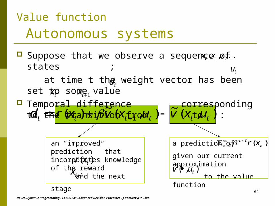
Autonomous systems Suppose that we observe a sequence of states ;
at time t the weight vector has been set to some value Temporal difference corresponding to the transition
from to :td
),(~),(~)( 1 tttttt uxvuxvxrd
....,, 210 xxx
tu
tx 1tx
a prediction of
given our current approximation
to the value function
)(
xrtt
),(~tuv
an “improved prediction ” that incorporates knowledge of the reward and the next
stage 1tx)( txr
Neuro-Dynamic Programming - ECECS 841- Advanced Decision Processes - J.Ramirez & Y. Liao
65
Value function
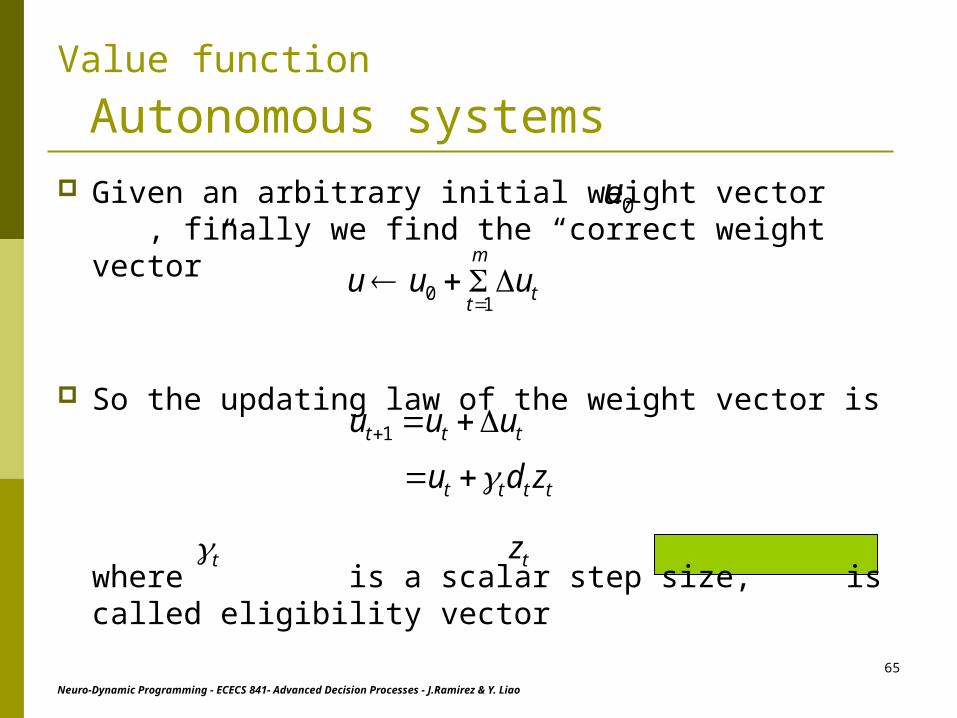
Autonomous systems Given an arbitrary initial weight vector , finally we find
the “correct weight vector”
So the updating law of the weight vector is
where is a scalar step size, is called eligibility vector
0u
t
m
tuuu
10
ttt uuu 1
tttt zdu
t tz

Neuro-Dynamic Programming - ECECS 841- Advanced Decision Processes - J.Ramirez & Y. Liao
66
Value function
Autonomous systems Eligibility vector is defined as
where
),(~)(0
uxvz ut
t
t
)()(0
xt
t
uu uxv ),(~ )()(
1 xku k
K
k
))(),...(( 1 xx K
)( x
providing a direction for the adjustment of such that
moves towards the improved prediction
tu),(~
tt uxv

Neuro-Dynamic Programming - ECECS 841- Advanced Decision Processes - J.Ramirez & Y. Liao
67
Value function
Autonomous systems Note that the eligibility vectors can be recursively updated
according to
)(
)()()(
)( )()(
)()()()(
)()(
)(
1
10
10
1
1)1(1
0
1
1
0
11
11
tt
t
tt
t
tt
ttt
tt
tt
t
ttt
xz
xx
xx
xx
xz
xzz

Neuro-Dynamic Programming - ECECS 841- Advanced Decision Processes - J.Ramirez & Y. Liao
68
Consequently, when the updating law of the weight vector can be rewritten as:
That means, only the last state has effect on the update In the more general case of ,
)()(0
1
xduu t
t
tttt
Value function
Autonomous systems
,0
)),(~),(~)()(( 11 ttttttttt uxvuxvxrxuu
]1,0(
“trigger”step size direction
Neuro-Dynamic Programming - ECECS 841- Advanced Decision Processes - J.Ramirez & Y. Liao
69
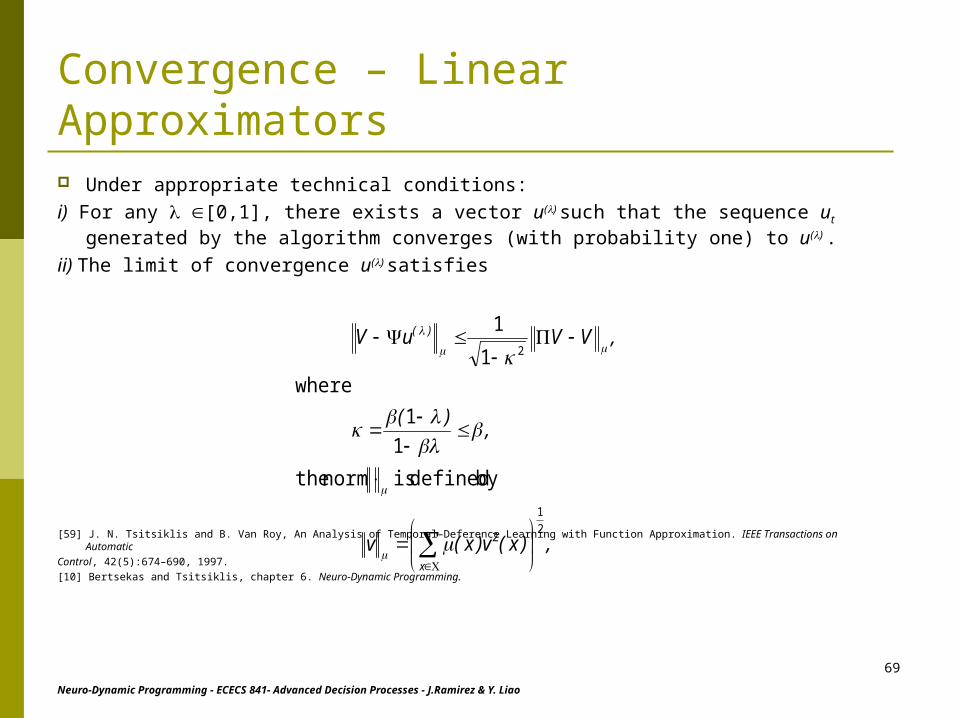
Convergence – Linear Approximators Under appropriate technical conditions:
i) For any [0,1], there exists a vector u() such that the sequence ut generated by the algorithm converges (with probability one) to u() .
ii) The limit of convergence u() satisfies
[59] J. N. Tsitsiklis and B. Van Roy, An Analysis of Temporal–Deference Learning with Function Approximation. IEEE Transactions on Automatic
Control, 42(5):674–690, 1997.
[10] Bertsekas and Tsitsiklis, chapter 6. Neuro-Dynamic Programming.
,)x(v)x(v
,)(
,VVuV
x
)(
2
1
2
2
by defined is norm the
1
1
where1
1
Neuro-Dynamic Programming - ECECS 841- Advanced Decision Processes - J.Ramirez & Y. Liao
70
Value function
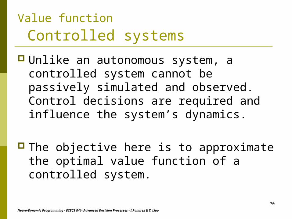
Controlled systems
Unlike an autonomous system, a controlled system cannot be passively simulated and observed. Control decisions are required and influence the system’s dynamics.
The objective here is to approximate the optimal value function of a controlled system.

Neuro-Dynamic Programming - ECECS 841- Advanced Decision Processes - J.Ramirez & Y. Liao
71
Approximate Policy Iteration A classical dynamic programming algorithm - policy iteration
Given a value function corresponding to a stationary policy
, an improved policy can be defined by
In particular, for all . Furthermore, a sequence of policies initialized
with some arbitrary and updated according to
converges to an optimal policy .
Value function
Controlled systems
),( v
*
0
)),,,((),(maxarg waxfvaxrx wa
),(),( xvxv Xx ,...2,1,0mm
)),,,((),(maxarg1 mwa
m waxfvaxrx
Neuro-Dynamic Programming - ECECS 841- Advanced Decision Processes - J.Ramirez & Y. Liao
72
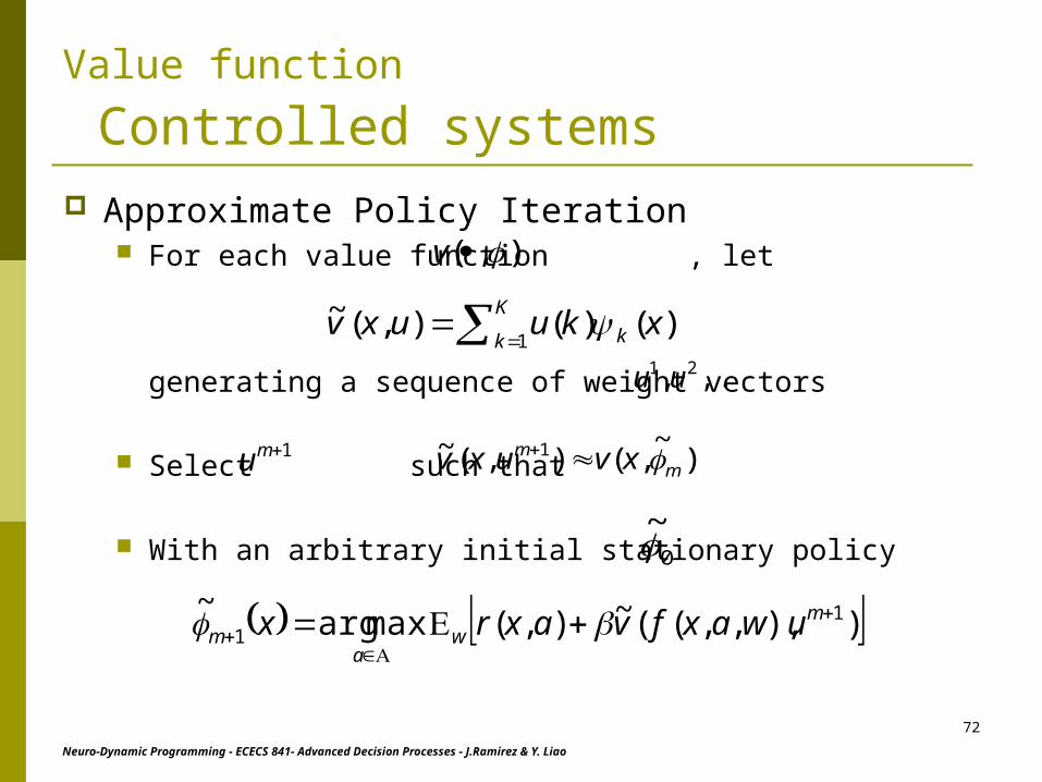
Value function
Controlled systems Approximate Policy Iteration
For each value function , let
generating a sequence of weight vectors
Select such that
With an arbitrary initial stationary policy
),( v
)),,,((~),(maxarg~ 1
1
m
wa
m uwaxfvaxrx
K
k k xkuuxv1
)()(),(~ ,..., 21 uu
1mu )~
,(),(~ 1m
m xvuxv
0
~

Neuro-Dynamic Programming - ECECS 841- Advanced Decision Processes - J.Ramirez & Y. Liao
73
Value function
Controlled systems Approximate Policy Iteration
Two loops:
External: find converged weight vector update the present stationary policy
Internal: applying temporal-difference learning to generate each iterate weight vector value function approximation
Initialization:mm uu 1
0

Neuro-Dynamic Programming - ECECS 841- Advanced Decision Processes - J.Ramirez & Y. Liao
74
Value function
Controlled systems Approximate Policy Iteration
A result from section 6.2 [10] D. P. Bertsekas and J. N. Tsitsiklis, Neuro-Dynamic Programming. Athena Scientific, Bellmont, MA, 1996.
if there exists some such that for all m
then
The external sequence does not always converge.
0
),())((max 1m
m
Xxxvxu
2)1(
2)())((maxsuplim
xVxum
Xxm
Neuro-Dynamic Programming - ECECS 841- Advanced Decision Processes - J.Ramirez & Y. Liao
75
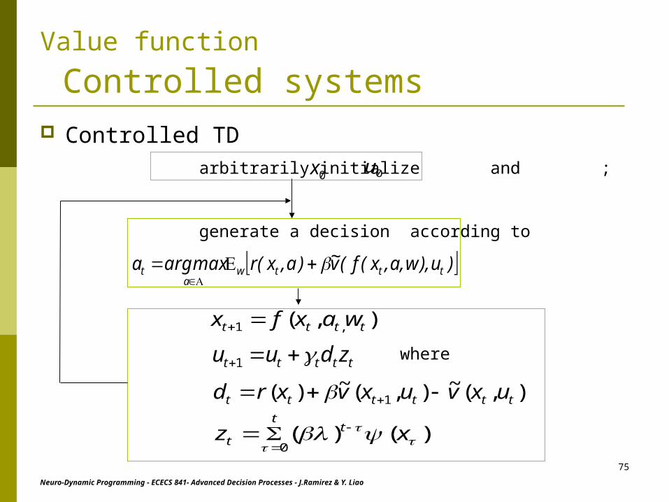
Controlled TD
arbitrarily initialize and ;
generate a decision according to
where
Value function
Controlled systems
0u0x
)u),w,a,x(f(v~)a,x(rmaxarga tttwa
t
),( ,1 tttt waxfx
),(~),(~)( 1 tttttt uxvuxvxrd ttttt zduu 1
)()(0
xz t
t
t

Neuro-Dynamic Programming - ECECS 841- Advanced Decision Processes - J.Ramirez & Y. Liao
76
Value function
Controlled systems Big problem: Convergence
A modification that has been found to be useful in practical applications involves adding “exploration noise” to the controls.
One approach to this end involves randomizing decisions by choosing at each time t a decision ,for , with probability
where is a small scalar.
aat Aat
Aa tttw
tttw
)/))u),w,a,x(f(v~)a,x(rexp((
)/))u),w,a,x(f(v~)a,x(rexp((
0

Neuro-Dynamic Programming - ECECS 841- Advanced Decision Processes - J.Ramirez & Y. Liao
77
Value function
Controlled systemsNote: 1) Probability >0
2) , the probability of ,such that
simple proof:
0 ta 1
)u),w,a,x(f(v~)a,x(rmaxarga tttwa
t
1
)/))),,,((~),()),,,((~),(exp((
1lim
)/))),,,((~),()),,,((~),(exp((*)/))),,,((~),(exp((
)/))),,,((~),(exp((lim
)/))),,,((~),(exp((
)/))),,,((~),(exp((lim
0
0
0
Aa tttwtttw
Aa tttwtttwtttw
tttw
Aa tttw
tttw
uwaxfvaxruwaxfvaxr
uwaxfvaxruwaxfvaxruwaxfvaxr
uwaxfvaxr
uwaxfvaxr
uwaxfvaxr

Neuro-Dynamic Programming - ECECS 841- Advanced Decision Processes - J.Ramirez & Y. Liao
78
Q-Function Given V,
Define a Q-function:
then
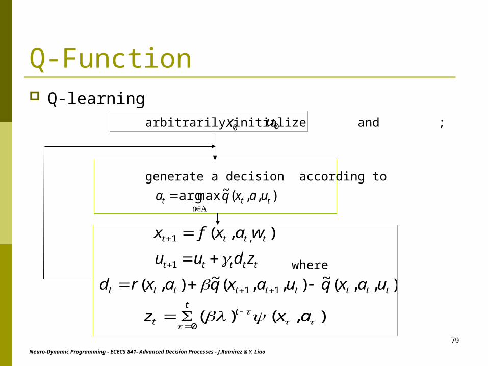
Q–learning is a variant of temporal–difference learning that approximates Q functions rather than value functions.
))w,a,x(f(V)a,x(rmaxarga ttwa
t
))w,a,x(f(V)a,x(r)a,x(Q ttw
),(maxarg axQa ta
t
),()(),,(~),(1
axkuuaxqaxQ k
K
k
Neuro-Dynamic Programming - ECECS 841- Advanced Decision Processes - J.Ramirez & Y. Liao
79
Q-learning
arbitrarily initialize and ;
generate a decision according to
where
Q-Function
0u0x
),,(~maxarg tta
t uaxqa
),( ,1 tttt waxfx
),,(~),,(~),( 11 ttttttttt uaxquaxqaxrd ttttt zduu 1
),()(0
axz t
t
t

Neuro-Dynamic Programming - ECECS 841- Advanced Decision Processes - J.Ramirez & Y. Liao
80
Q-Function Like in the case of controlled TD, it is often desirable to incorporate exploration. Randomize decisions by choosing at each time t a decision ,for , with
probability
where is a small scalar.Note: 1) Probability >0
2) , the probability of ,such that
The analysis of Q–learning bears many similarities with that of controlled TD, and results that apply to one can often be generalized in a straightforward way to accommodate the other.
aat Aat
Aa tt
tt
uaxq
uaxq
)/),,(~exp(
)/),,(~exp(
0
0 ta 1
),,(~maxarg tta
t uaxqa

Neuro-Dynamic Programming - ECECS 841- Advanced Decision Processes - J.Ramirez & Y. Liao
81
Relationship with Approximate Value Iteration
The classical value iteration algorithm can be described compactly in terms of the “dynamic programming operator” T,
Approximate Value iteration:
Disadvantage: the approximate value iteration need not possess fixed points, and
therefore should not be expected to converge. In fact, even in cases where a fixed point exists, and even when the
system is autonomous, the algorithm can generate a diverging sequence of weight vectors.
)),,((),(max)( waxfvwxrxTv wa
Dkk
Ruuvkk uvuvTuvTuv
kuk
1}{,~
1 ,~,~minarg,~,~
1

Neuro-Dynamic Programming - ECECS 841- Advanced Decision Processes - J.Ramirez & Y. Liao
82
Relationship with Approximate Value Iteration
V
),(~0uv
),(~0uvT
),(~1uv
min
),(~1uvT
),(~2uv

Neuro-Dynamic Programming - ECECS 841- Advanced Decision Processes - J.Ramirez & Y. Liao
83
Relationship with Approximate Value Iteration
Controlled TD can be thought of as a stochastic approximation algorithm designed to converge on fixed points of approximate value iteration.
Advantage:
Controlled TD uses simulation to effectively bypass the need to explicitly compute projections required for approximate value iteration. Autonomous systems
Controlled systems: the possible introduction of exploration

Neuro-Dynamic Programming - ECECS 841- Advanced Decision Processes - J.Ramirez & Y. Liao
84
Historical View A long history and big names
Sutton: Temporal–difference based on earlier work by Barto and Sutton on models for classical conditioning phenomena observed in animal behavior and by Barto, Sutton, and Anderson on “actor–critic methods”
Witten: look–up table algorithm bears similarities with one proposed a decade earlier.
Watkins: Q–learning was propose in his thesis; and the study of temporal–dierence learning was integrated with classical ideas from dynamic programming and stochastic approximation theory.
The work of Werbos and Barto, Bradtke, and Singh also contributed to the above integration.

Neuro-Dynamic Programming - ECECS 841- Advanced Decision Processes - J.Ramirez & Y. Liao
85
Historical View Application
Tesauro: a world–class Backgammon playing program. The practical potential was first demonstrated since then
channel allocation in cellular communication networks elevator dispatching inventory management job–shop scheduling

Neuro-Dynamic Programming - ECECS 841- Advanced Decision Processes - J.Ramirez & Y. Liao
86
Actors and Critics: Averaged Rewards
Independent actors
An actor is a parameterized class of policies.
))(,(
1lim)(
1tt
N
tNxxrE
Nv
lR

Neuro-Dynamic Programming - ECECS 841- Advanced Decision Processes - J.Ramirez & Y. Liao
87
Independent actors (cont.)
one stochastic gradient method, which was proposed by Marbach and Tsitsiklis
where
Using critic Feedback
Actors and Critics:
mmm
mmmm
r
1
11
)(
)(ˆ
m
m m
m
t
tt tt
tttm xa
xaq
an estimate of the
gradient given
parameters
1
)),((ˆm
m
t
tmt raxrq
K
kk axkuuaxq
1
),()(),,(~

Neuro-Dynamic Programming - ECECS 841- Advanced Decision Processes - J.Ramirez & Y. Liao
88

Neuro-Dynamic Programming - ECECS 841- Advanced Decision Processes - J.Ramirez & Y. Liao
89
Bibliography [1] D. P. Bertsekas, Dynamic Programming and Optimal Control. Athena
Scientific, Bellmont, MA, 1995. [2] D. P. Bertsekas and J. N. Tsitsiklis, Neuro-Dynamic Programming.
Athena Scientific, Bellmont, MA, 1996. [3] R. S. Sutton, Temporal Credic Assignment in Reinforcement Learning.
PhD thesis, University of Massachusetts, Amherst, Amherst, MA, 1984. [4] R. S. Sutton, Learning to Predict by the Methods of Temporal
Differences. Machine Learning, 3:9–44, 1988. [5] R. S. Sutton and A. G. Barto, Reinforcement Learning: An
Introduction.MIT Press, Cambridge, MA, 1998.
[6] J. N. Tsitsiklis and B. Van Roy, An Analysis of Temporal–DierenceLearning with Function Approximation. IEEE Transactions on AutomaticControl, 42(5):674–690, 1997.