1

Network Metrics:A Network Analysis EngineICCS 2006 ConferenceJune 2006 Boston MA

Joseph E. Johnson, PhD

Department of Physics

University of South Carolina

jjohnson@sc.edu

June 22, 2006 ©

2

Executive Overview Networks are extremely difficult to track We have discovered new network metrics These metrics can be used with all networks Our algorithms detect network changes We seek to deploy our code in all domains

3

The Network Problem

Networks are ubiquitous and complex They are at the foundation of a large number

of mathematically unsolved problems Large networks are difficult to analyze and to

dynamically track. We have found an a promising set of metrics

that can be used to characterize networks

4

Executive Summary 1

Networks: defined by a connection matrix Cij

We assign specific diagonal values Then M = eC is a Markov matrix M has columns are probability distributions We compute generalized column entropies

5

Executive Summary 2

The spectral curve characterizes the network’s topological structure

Determine ‘normal’ spectra Identify nodes that are topologically aberrant

6

Executive Summary 3

Do this for both columns and rows Network behavior can be further reduced Use 3 parameters track deviancy from normal We have developed algorithms in JAVA and

Mathematica

7

The Technical Details

8

Our Insights to be here presented – We will show that:

I: Networks are 1-1 with Markov transformations. II: Conserved Markov network flows track topology III. Compute entropy functions on Markov matrices IV: 2N entropy spectra proposed as network metrics V: Our software algorithms are general purpose VI: A totally solid mathematics & intuitive model

9

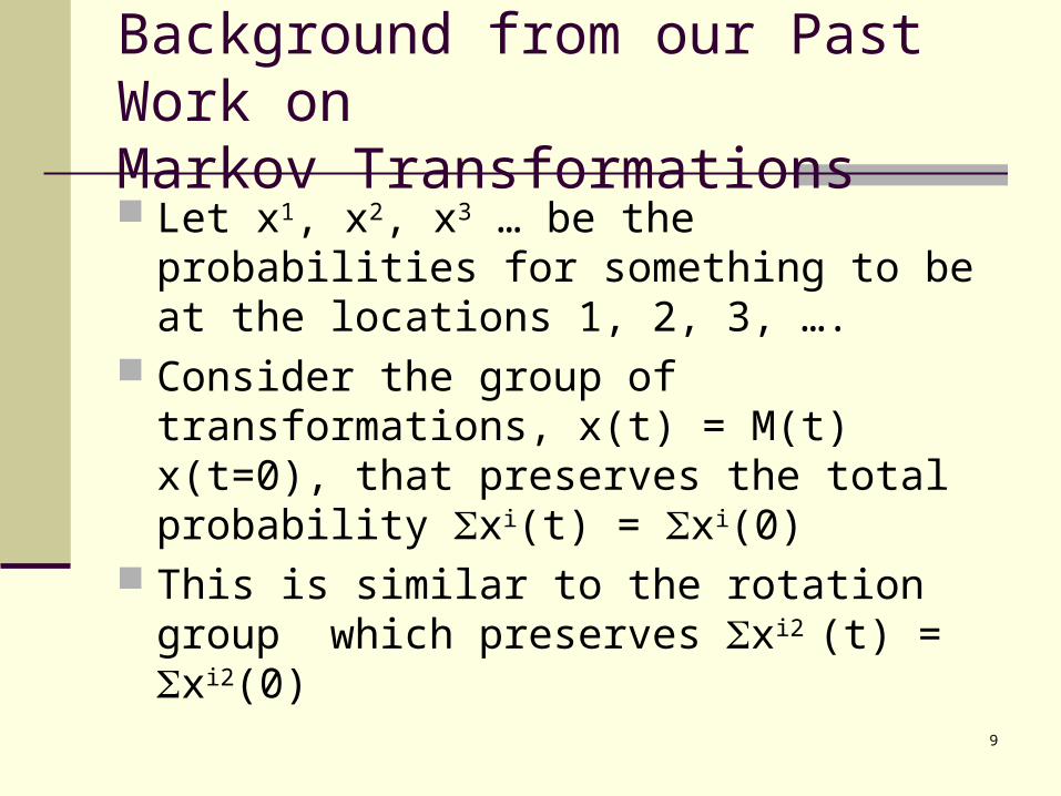
Background from our Past Work on Markov Transformations Let x1, x2, x3 … be the probabilities for

something to be at the locations 1, 2, 3, …. Consider the group of transformations, x(t) =

M(t) x(t=0), that preserves the total probability xi(t) = xi(0)

This is similar to the rotation group which preserves xi2 (t) = xi2(0)

10

An Example:

Einstein – random walk, diffusion theory 1905 Markov (1906) transformations (80% probable to stay put

and 10% probable to move to the two adjacent cells): |X’> = M |X> can be written as (note columns sum to unity):

0 0.8 0.1 0 0 0.1 0

0.1 0.1 0.8 0.1 0 0 0

0.8 0 0.1 0.8 0.1 0 1

0.1 0 0 0.1 0.8 0.1 0

0 0.1 0 0 0.1 0.8 0

Example of a discrete Markov transformation.

Note the irreversible diffusion.

11

GL(n,R) – Lie Algebra Decomposition

The N2 matrices with a 1 at the i,j position, and 0 elsewhere, form a basis of GL(n,R)

Matrices with a ‘1’ at the ij position and a -1 on the diagonal at jj can be shown to close into a (Markov type) Lie Algebra and still form a basis of the off-diagonal matrices.

Matrices with only a ‘1’ on a diagonal position are a complete basis for the Abelian scaling Lie group.

All general linear transformations are decomposable into these two Lie groups: Markov type & scaling.

12

Define the Lie Algebra for Markov Transformations The Markov Lie Group is defined by transformations that

preserve the sum of the elements of a vector ie xi’ = xi

The generators are defined by ‘rob Peter to pay Paul’ for M = et L where L= ijijLij is defined by the summation over L with a ‘1’ in row i and column j along with a ‘-1’ in the diagonal position row j and column j

In two dimensions we get:

L12 = L21 = 1 0

1 0

0 1

0 1

0 1

0 1

13

Lie group defined:

And the Markov group transformation then takes the form: M(t) = e s =

One notes that the column sums are unity as is required for a Markov transformation.

This transformation gradually transforms the x2 value into the x1 value preserving x1 + x2 = constant.

0 1

0 1

1 1

0

s

s

e

e

14

Higher Dimensions:

This Markov Lie Algebra can be defined on spaces of all integral dimensions (2, 3,….) and has n2 - n generators for n dimensions representing basis elements with a ‘1’ in the ij position and a ‘-1’ in the jj position.

This makes this basis a complete basis for all off-diagonal matrices. E.g. in 5 dimensions:

L14 = 0 0 0 1 0

0 0 0 0 0

0 0 0 0 0

0 0 0 1 0

0 0 0 0 0

15

Graphically, One can Visualize This

These transformations in two dimensions define the group of motions on a straight line.

The Markov Lie group is a mapping of this line back into itself – but is NOT a translation group.

In generally one gets hyperplane motions.

0

10

20

30

40

50

60

70

80

90

1st Qtr 2nd Qtr 3rd Qtr 4th Qtr

East

West

North

Y

-1.5

-1

-0.5

0

0.5

1

1.5

2

2.5

3

3.5

-2.5 -2 -1.5 -1 -0.5 0 0.5 1 1.5 2 2.5

Y

16

Loss of the Markov Inverse giving a Lie monoid To be probabilities, non-negative values must

be transformed into nonnegative values This exactly removes all inverses Allowable transformations are those with non-

negative linear combinations This gives us a Lie Monoid & Irreversibility.

17

Our New Applications to Networks

18

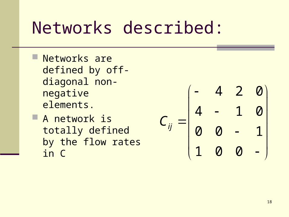
Networks described:

Networks are defined by off-diagonal non-negative elements.

A network is totally defined by the flow rates in C

4 2 0

4 1 0

0 0 1

1 0 0

ijC

19

Network topologies are 1-1 with Markov Lie generators The Lie monoid basis for transformations is

identical to a connection matrix where the diagonals are set to the negative of the sum of other values.

Thus network topologies are then 1-1 with Markov Lie generators

Every possible network corresponds to exactly one Markov family of transformations

20

Entropies can be computed on column probability densities Markov matrix columns are probabilities

Actually this holds to any order of expansion of M=eC if care is taken to use small

Thus we can compute entropy on each column distributions. We prefer to use second order Renyi entropy:

log2 (N(xi2))

21

Asymmetry gives more information

Asymmetry detection in the network is important

This asymmetry results in two spectral entropy curves – one for rows and one for columns

22

Spectral curve from sorted entropies

We only care about the overall pattern Thus entropies are sorted in order to derive a

spectral curve At each window of time, the sorting is redone

23

Normal & Anomalous Spectra

Spectral form studied relative to normal Correlation to normal studied by many

methods such as sums of squares of differences between current and normal entropy

Two values now represent the network at a given time: row and column sum of squares deviation from the normal

Wavelets and other expansions can be used on the spectra

24

Underlying Interpretation and Model

1 to 1 correspondence: one network to one family of Markov transformations.

The interpretation of M is a conserved flow Flows are at the rates indicated in C

25

Entropy Interpretation of the Flows

The altered C matrix is evolving family of Markov conserved flows corresponding exactly to the topology.

The entropy encapsulates the order/disorder of that nodes topology.

The entire spectra captures the entire order and disorder for the entire network

26

Eigenvalue Interpretation

The eigenvalues of C are rates of approach to equilibrium of a conserved fluid (probability) – like normal modes .

The eigenvectors are linear combinations of nodes that have simple exponential decays

27

Interpretation of Generalized Entropy

x(i) has a high degree of information (order) when it is concentrated in one area

The integral of the squares is maximum when x(i) is concentrated.

To obtain addativity of independent systems, we define the negative entropy (information) as I = log2(Nxi2)

28

Entropy used as a metric

The entropy spectra is the order associated with the distributed transfer

A random uniform distribution to all nodes gives high entropy while an organized transfer to a few nodes give low entropy.

The entropy function is thus measuring the order associated with transfer process.

29

Other Choices of Diagonal Values

Any diagonal value can be inserted into the generator from the scaling group.

Such action is equivalent to providing a source or sink of the conserved probability fluid at that node by the amount of deviation from the Markov value.

30

Abelian Scaling Group

Consider the Abelian scaling group generated by Lii = 1:

When adjoined to the Markov group, one obtains the entire general linear group, GL(n,R).

It is obvious that the combined Lie algebra spans all n x n matrices.

0 0 0 0

0 1 0 0

0 0 0 0

0 0 0 0

1 0 0 0

0 0 0

0 0 1 0

0 0 0 1

ssee

31

Practical Application -1

Use Time, Node i, Node j, and weight for C Fix diagonals for Markov generation. Normalize C matrix Adjust Compute M to a given order of expansion

32

Practical Application - 2

Compute entropy for each column of M Sort entropies to obtain a spectral curve Establish the ‘normal’ distribution

33

Practical Application - 3

Compute/display current-normal entropy spectral

Compute the sums of squares of deviations Do all this also for rows

34

Software Applications to Network Monitoring

35

Process

Network represented by two entropy spectral curves for incoming and outgoing links.

They represent entropy of a conserved fluid flow on that topology

Eigenvectors and eigenvalues have clear interpretation.

36

Software Functionality

Software is general purpose Normality for that network is established

37

Normal spectra is subtracted from the current distribution.

The network is thus reduced to two values whose deviation from normal is tracked

38

Utility of the algorithm

We seek to test the utility of these algorithms in all network domains.

Patents have been filled on these processes by the University of South Carolina

39

Thank You

40

41

42

Examples of Networks:

Communication Networks The Internet Phone (wired & wireless) Mail, Fed-Ex, UPS

Transportation Networks Air Traffic Highways Waterway Railroads Pipelines

43

More Examples:

Financial Networks Banking & Fund Transfers Accounting Flows Ownership & Investments Input-Output Economic Flows

Utility & Energy Networks Electrical Power Grids Electrical Circuits & Devices Water & Sewer Flows Natural Gas Distribution

Biological Networks esp. Disease Contagious Diseases Neural Nets

44

Markov Theory

“Markov Type Lie Groups in GL(n,R)”, Joseph E Johnson, 1985, J Math. Phys.

GL(n,R) = M(n,R) + A(n,R) Then M(n,R) = MM(n,R) + their inverses

where MM refers to the Markov Monoid MM contain diffusion, entropy, & irreversibility

45

46

Unanswered Questions for Further Research ** The window of time when chosen too short

gives low entropy as it does not reflect the true distribution of the connections.

The entropy is not additive from one time to another i.e. 2 windows taken as 1 window does not give a linear composition of the combined entropy.

**What spectral curves are possible – derive them.