1

Monopolistic Competition and

Oligopoly

Chapter 10

2

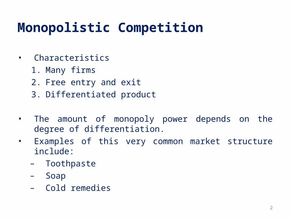
Monopolistic Competition

• Characteristics1. Many firms2. Free entry and exit3. Differentiated product

• The amount of monopoly power depends on the degree of differentiation.

• Examples of this very common market structure include:

– Toothpaste– Soap– Cold remedies

3

• Toothpaste– Crest and monopoly power

• Procter & Gamble is the sole producer of Crest• Consumers can have a preference for Crest – taste,

reputation, decay preventing efficacy• The greater the preference (differentiation) the

higher the price.

• Two important characteristics– Differentiated but highly substitutable

products– Free entry and exit

4

A Monopolistically CompetitiveFirm in the Short and Long Run

Quantity

$/Q

Quantity

$/QMC

AC

MC

AC

DSR

MRSR

DLR

MRLR

QSR

PSR

QLR

PLR

Short Run Long Run

5

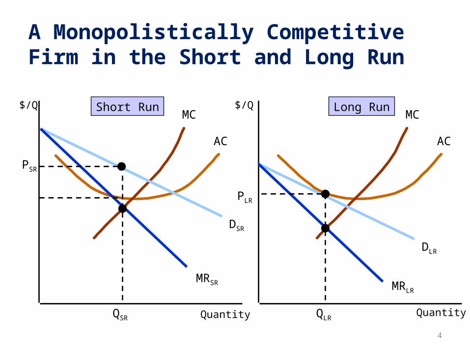
A Monopolistically CompetitiveFirm in the Short and Long Run

• Short-run– Downward sloping demand –

differentiated product– Demand is relatively elastic – good

substitutes– MR < P– Profits are maximized when MR = MC– This firm is making economic profits

6

A Monopolistically CompetitiveFirm in the Short and Long Run

• Long-run– Profits will attract new firms to the

industry (no barriers to entry)– The old firm’s demand will decrease to

DLR– Firm’s output and price will fall– Industry output will rise– No economic profit (P = AC)– P > MC some monopoly power

7

Oligopoly – Characteristics

• Small number of firms• Product differentiation may or may not exist• Barriers to entry

– Scale economies– Patents– Technology– Name recognition– Strategic action

• Examples– Automobiles– Steel– Aluminum– Petrochemicals– Electrical equipment

8

Oligopoly – Equilibrium• If one firm decides to cut their price, they must consider

what the other firms in the industry will do– Could cut price some, the same amount, or more than

firm– Could lead to price war and drastic fall in profits for all

• Actions and reactions are dynamic, evolving over time

• Defining Equilibrium– Firms are doing the best they can and have no incentive

to change their output or price– All firms assume competitors are taking rival decisions

into account.• Nash Equilibrium

– Each firm is doing the best it can given what its competitors are doing.

• We will focus on duopoly– Markets in which two firms compete

9

Oligopoly

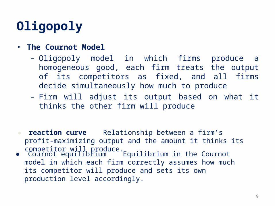
• The Cournot Model– Oligopoly model in which firms produce a homogeneous

good, each firm treats the output of its competitors as fixed, and all firms decide simultaneously how much to produce

– Firm will adjust its output based on what it thinks the other firm will produce

● reaction curve Relationship between a firm’s profit-maximizing output and the amount it thinks its competitor will produce.

● Cournot equilibrium Equilibrium in the Cournot model in which each firm correctly assumes how much its competitor will produce and sets its own production level accordingly.

10

Oligopoly

• The Reaction Curve– The relationship between a firm’s profit-

maximizing output and the amount it thinks its competitor will produce.

– A firm’s profit-maximizing output is a decreasing schedule of the expected output of Firm 2.

11

Reaction Curves and Cournot Equilibrium

Firm 2’s ReactionCurve Q*2(Q2)

Q225 50 75 100

25

50

75

100

Firm 1’s ReactionCurve Q*1(Q2)

x

x

x

x

Firm 1’s reaction curve shows how much itwill produce as a function of how much it thinks Firm 2 will produce. The x’s

correspond to the previous model.

Firm 2’s reaction curve shows how much itwill produce as a function of how much

it thinks Firm 1 will produce.

12

The Linear Demand Curve

• An Example of the Cournot Equilibrium– Two firms face linear market demand curve– We can compare competitive equilibrium and

the equilibrium resulting from collusion– Market demand is P = 30 - Q – Q is total production of both firms: – Q = Q1 + Q2– Both firms have MC1 = MC2 = 0

13

Oligopoly Example

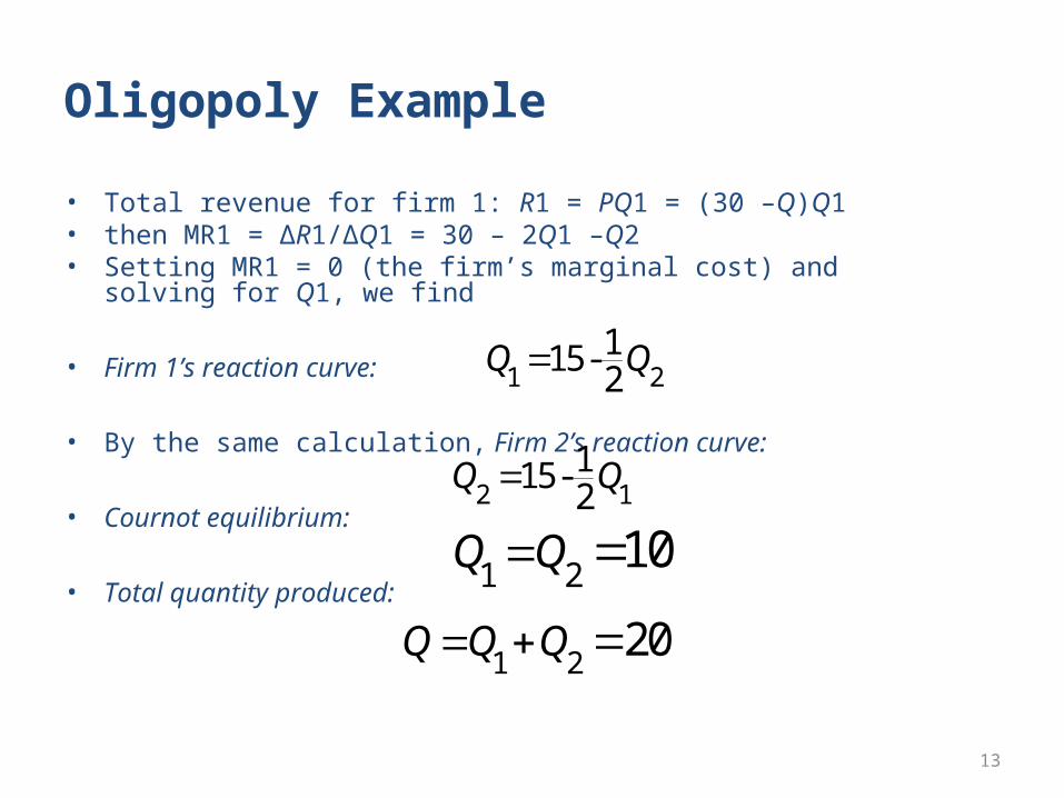
• Total revenue for firm 1: R1 = PQ1 = (30 –Q)Q1• then MR1 = ∆R1/∆Q1 = 30 – 2Q1 –Q2• Setting MR1 = 0 (the firm’s marginal cost) and solving for Q1,

we find

• Firm 1’s reaction curve:

• By the same calculation, Firm 2’s reaction curve:

• Cournot equilibrium:

• Total quantity produced:

1 2115-2

Q Q

2 1115-2

Q Q

1 210Q Q

1 220Q Q Q

14

Oligopoly Example

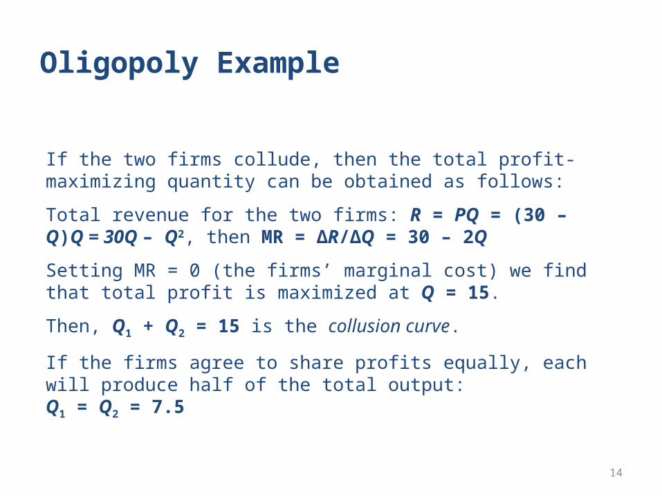
If the two firms collude, then the total profit-maximizing quantity can be obtained as follows:

Total revenue for the two firms: R = PQ = (30 –Q)Q = 30Q – Q2, then MR = ∆R/∆Q = 30 – 2Q

Setting MR = 0 (the firms’ marginal cost) we find that total profit is maximized at Q = 15.

Then, Q1 + Q2 = 15 is the collusion curve.

If the firms agree to share profits equally, each will produce half of the total output:Q1 = Q2 = 7.5

15

First Mover Advantage – The Stackelberg Model

• Oligopoly model in which one firm sets its output before other firms do.

• Assumptions– One firm can set output first– MC = 0– Market demand is P = 30 - Q where Q is total

output– Firm 1 sets output first and Firm 2 then makes an

output decision seeing Firm 1 output• Firm 1– Must consider the reaction of Firm 2

• Firm 2– Takes Firm 1’s output as fixed and therefore

determines output with the Cournot reaction curve: Q2 = 15 - ½(Q1)

16

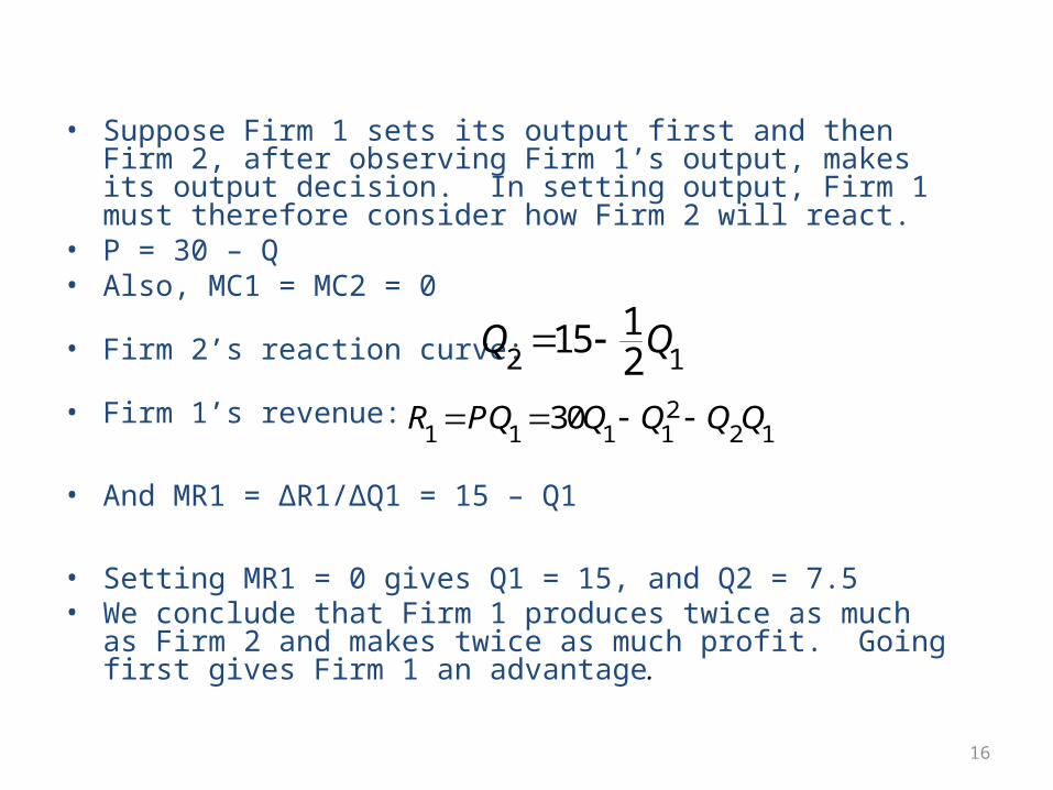
• Suppose Firm 1 sets its output first and then Firm 2, after observing Firm 1’s output, makes its output decision. In setting output, Firm 1 must therefore consider how Firm 2 will react.

• P = 30 – Q• Also, MC1 = MC2 = 0

• Firm 2’s reaction curve:

• Firm 1’s revenue:

• And MR1 = ∆R1/∆Q1 = 15 – Q1

• Setting MR1 = 0 gives Q1 = 15, and Q2 = 7.5• We conclude that Firm 1 produces twice as much as Firm

2 and makes twice as much profit. Going first gives Firm 1 an advantage.

2 11152

Q Q

21 1 1 1 2 1

30R PQ Q Q Q Q

17

Price CompetitionCompetition in an oligopolistic industry may occur with price instead of output.

The Bertrand Model is used

Oligopoly model in which firms produce a homogeneous good, each firm treats the price of its competitors as fixed, and all firms decide simultaneously what price to charge

AssumptionsHomogenous goodMarket demand is P = 30 - Q where Q = Q1 + Q2MC1 = MC2 = $3

Can show the Cournot equilibrium if Q1 = Q2 = 9 and market price is $12 giving each firm a profits of $81.

18

Price Competition – Bertrand Model

• Assume here that the firms compete with price, not quantity.

• Since good is homogeneous, consumers will buy from lowest price seller– If firms charge different prices, consumers buy from

lowest priced firm only– If firms charge same price, consumers are indifferent

who they buy from• Nash equilibrium is competitive output since have

incentive to cut prices• Both firms set price equal to MC

– P = MC; P1 = P2 = $3– Q = 27; Q1 & Q2 = 13.5

• Both firms earn zero profit

19

Price Competition – Differentiated Products

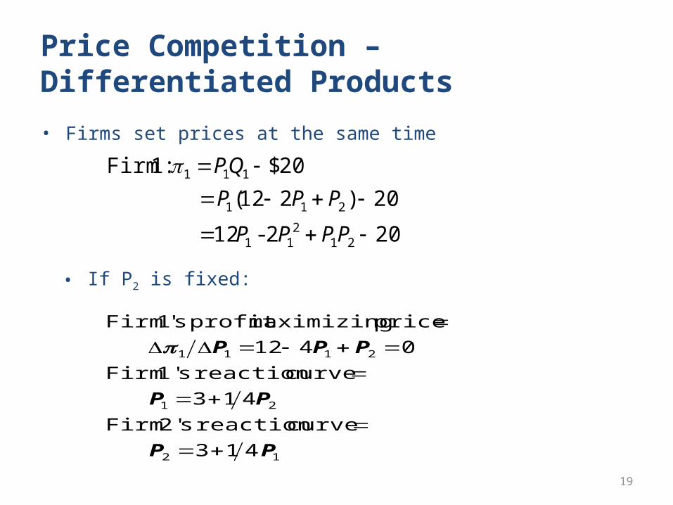
• Firms set prices at the same time

202-12

20)212(

20$ :1 Firm

212

11

211

111

PPPP

PPP

QP

• If P2 is fixed:

12

21

2111

413

413

0412

'

PP

PP

PPP

curve reaction s2' Firm

curve reaction s1' Firm

price maximizing profit s1 Firm

20

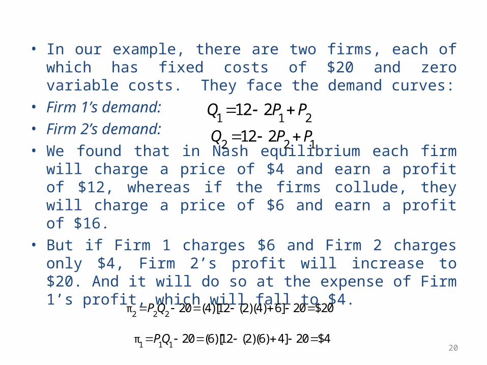
• In our example, there are two firms, each of which has fixed costs of $20 and zero variable costs. They face the demand curves:

• Firm 1’s demand:• Firm 2’s demand:• We found that in Nash equilibrium each firm will

charge a price of $4 and earn a profit of $12, whereas if the firms collude, they will charge a price of $6 and earn a profit of $16.

• But if Firm 1 charges $6 and Firm 2 charges only $4, Firm 2’s profit will increase to $20. And it will do so at the expense of Firm 1’s profit, which will fall to $4.

2 2 2π 20 (4)[12 (2)(4) 6] 20 $20PQ

1 1 1π 20 (6)[12 (2)(6) 4] 20 $4PQ

1 1 212 2Q P P

2 2 112 2Q P P

21

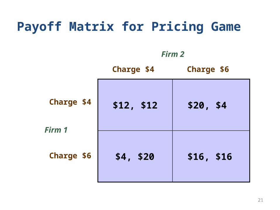
Payoff Matrix for Pricing Game

$12, $12 $20, $4

$16, $16$4, $20

Charge $4

Charge $4

Charge $6

Charge $6

Firm 2

Firm 1

22

• An example in game theory, called the Prisoners’ Dilemma, illustrates the problem oligopolistic firms face.– Two prisoners have been accused of collaborating in a

crime.– They are in separate jail cells and cannot communicate.– Each has been asked to confess to the crime.

-5, -5 -1, -10

-2, -2-10, -1

Confess Don’t confess

Confess

Don’tconfess

Would you choose to confess?Prisoner A

Prisoner B

23

Price Signaling and Price Leadership

• Price Signaling– Implicit collusion in which a firm announces a price

increase in the hope that other firms will follow suit• Price Leadership

– Pattern of pricing in which one firm regularly announces price changes that other firms then match

• The Dominant Firm Model– In some oligopolistic markets, one large firm has a

major share of total sales, and a group of smaller firms supplies the remainder of the market.

– The large firm might then act as the dominant firm, setting a price that maximizes its own profits.

24

The Dominant Firm Model

• Dominant firm must determine its demand curve, DD.– Difference between market demand and

supply of fringe firms• To maximize profits, dominant firm produces QD

where MRD and MCD cross.• At P*, fringe firms sell QF and total quantity sold

is QT = QD + QF

25

Cartels• Producers in a cartel explicitly agree to cooperate in setting

prices and output.• Typically only a subset of producers are part of the cartel

and others benefit from the choices of the cartel• If demand is sufficiently inelastic and cartel is enforceable,

prices may be well above competitive levels

• Examples of successful cartels– OPEC– International

Bauxite Association– Mercurio Europeo

• Examples of unsuccessful cartels– Copper– Tin– Coffee– Tea– Cocoa