1

Midterm Exam

• Mean: 72.7%

• Max: 100.25%

Histogram

0

1

2

3

4

5

6

7

8

9

Bin

Frequency

10090807060504030

Kernel Density Estimation

2

HW and Overall Grades

Homework AvgsMean = 78.9%

Grades So FarMean = 77.7%

The “grade so far” is based only on homeworks 1-4 and the midterm (~36% of the course grade). It does not include participation, or any project components.

ABCF / D(These letter grade breakdowns are a GUIDELINE ONLY and do not override the letter grade breakdown defined in the syllabus.)

3

Bayesian NetworksBayesian Networks

Chapter 14.1-14.2; 14.4

CMSC 471CMSC 471

Adapted from slides byTim Finin andMarie desJardins.

Some material borrowedfrom Lise Getoor.

4

Outline

• Bayesian networks– Network structure

– Conditional probability tables

– Conditional independence

• Inference in Bayesian networks– Exact inference

– Approximate inference

5

Bayesian Belief Networks (BNs)

• Definition: BN = (DAG, CPD) – DAG: directed acyclic graph (BN’s structure)

• Nodes: random variables (typically binary or discrete, but methods also exist to handle continuous variables)

• Arcs: indicate probabilistic dependencies between nodes (lack of link signifies conditional independence)

– CPD: conditional probability distribution (BN’s parameters)• Conditional probabilities at each node, usually stored as a table

(conditional probability table, or CPT)

– Root nodes are a special case – no parents, so just use priors in CPD:

iiii xxP of nodesparent all ofset theis where)|(

)()|( so , iiii xPxP

6

Example BN

a

b c

d e

P(C|A) = 0.2 P(C|A) = 0.005P(B|A) = 0.3

P(B|A) = 0.001

P(A) = 0.001

P(D|B,C) = 0.1 P(D|B,C) = 0.01P(D|B,C) = 0.01 P(D|B,C) = 0.00001

P(E|C) = 0.4 P(E|C) = 0.002

Note that we only specify P(A) etc., not P(¬A), since they have to add to one

7

• Conditional independence assumption–

where q is any set of variables (nodes) other than and its successors

– blocks influence of other nodes on and its successors (q influences onlythrough variables in )

– With this assumption, the complete joint probability distribution of all variables in the network can be represented by (recovered from) local CPDs by chaining these CPDs:

ix

)|(),...,( 11 iinin xPxxP

)|(),|( iiii xPqxP

ix i ix

i q

ix i

Conditional independence and chaining

8

Chaining: Example

Computing the joint probability for all variables is easy:

P(a, b, c, d, e) = P(e | a, b, c, d) P(a, b, c, d) by the product rule= P(e | c) P(a, b, c, d) by cond. indep. assumption= P(e | c) P(d | a, b, c) P(a, b, c) = P(e | c) P(d | b, c) P(c | a, b) P(a, b)= P(e | c) P(d | b, c) P(c | a) P(b | a) P(a)

a

b c

d e

9

Topological semantics

• A node is conditionally independent of its non-descendants given its parents

• A node is conditionally independent of all other nodes in the network given its parents, children, and children’s parents (also known as its Markov blanket)

• The method called d-separation can be applied to decide whether a set of nodes X is independent of another set Y, given a third set Z

11

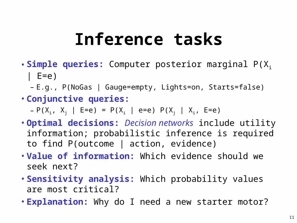
Inference tasks

• Simple queries: Computer posterior marginal P(Xi | E=e)– E.g., P(NoGas | Gauge=empty, Lights=on, Starts=false)

• Conjunctive queries: – P(Xi, Xj | E=e) = P(Xi | e=e) P(Xj | Xi, E=e)

• Optimal decisions: Decision networks include utility information; probabilistic inference is required to find P(outcome | action, evidence)

• Value of information: Which evidence should we seek next?

• Sensitivity analysis: Which probability values are most critical?

• Explanation: Why do I need a new starter motor?

12

Approaches to inference

• Exact inference – Enumeration

– Belief propagation in polytrees

– Variable elimination

– Clustering / join tree algorithms

• Approximate inference– Stochastic simulation / sampling methods

– Markov chain Monte Carlo methods

– Genetic algorithms

– Neural networks

– Simulated annealing

– Mean field theory

13

Direct inference with BNs

• Instead of computing the joint, suppose we just want the probability for one variable

• Exact methods of computation:– Enumeration

– Variable elimination

• Join trees: get the probabilities associated with every query variable

14

Inference by enumeration

• Add all of the terms (atomic event probabilities) from the full joint distribution

• If E are the evidence (observed) variables and Y are the other (unobserved) variables, then:

P(X|e) = α P(X, E) = α ∑ P(X, E, Y)

• Each P(X, E, Y) term can be computed using the chain rule

• Computationally expensive!

15

Example: Enumeration

• P(xi) = Σ πi P(xi | πi) P(πi)

• Suppose we want P(D=true), and only the value of E is given as true

• P (d|e) = ΣABCP(a, b, c, d, e) = ΣABCP(a) P(b|a) P(c|a) P(d|b,c) P(e|c)

• With simple iteration to compute this expression, there’s going to be a lot of repetition (e.g., P(e|c) has to be recomputed every time we iterate over C=true)

a

b c

d e

16

Exercise: Enumeration

smart study

prepared fair

pass

p(smart)=.8 p(study)=.6

p(fair)=.9

p(prep|…) smart smart

study .9 .7

study .5 .1

p(pass|…)smart smart

prep prep prep prep

fair .9 .7 .7 .2

fair .1 .1 .1 .1

Query: What is the probability that a student studied, given that they pass the exam?

45

Summary

• Bayes nets– Structure

– Parameters

– Conditional independence

– Chaining

• BN inference– Enumeration

– Variable elimination

– Sampling methods