
1 Managing Multi-Granular Linguistic Distribution ... · Group decision making (GDM) is a common...
32
arXiv:1504.01004v2 [cs.AI] 18 Nov 2015 1 Managing Multi-Granular Linguistic Distribution Assessments in Large-Scale Multi-Attribute Group Decision Making Zhen Zhang Member, IEEE, Chonghui Guo and Luis Mart´ ınez Member, IEEE Abstract Linguistic large-scale group decision making (LGDM) problems are more and more common nowadays. In such problems a large group of decision makers are involved in the decision process and elicit linguistic information that are usually assessed in different linguistic scales with diverse granularity because of decision makers’ distinct knowledge and background. To keep maximum information in initial stages of the linguistic LGDM problems, the use of multi-granular linguistic distribution assessments seems a suitable choice, however to manage such multi- granular linguistic distribution assessments, it is necessary the development of a new linguistic computational approach. In this paper it is proposed a novel computational model based on the use of extended linguistic hierarchies, which not only can be used to operate with multi-granular linguistic distribution assessments, but also can provide interpretable linguistic results to decision makers. Based on this new linguistic computational model, an approach to linguistic large-scale multi-attribute group decision making is proposed and applied to a talent selection process in universities. Index Terms group decision making (GDM), large-scale GDM, multi-granular linguistic information, linguistic distribution assessment. Manuscript received XX-XX-XXXX; revised XX-XX-XXXX; accepted XX-XX-XXXX. This work was partly supported by the National Natural Science Foundation of China (Nos. 71501023, 71171030), the Funds for Creative Research Groups of China (No. 71421001), the China Postdoctoral Science Foundation (2015M570248) and the Fundamental Research Funds for the Central Universities (DUT15RC(3)003) and by the Research Project TIN2015-66524 and FEDER funds Z. Zhang and C. Guo are with the Institute of Systems Engineering, Dalian University of Technology, Dalian 116024, China. E-mails: [email protected] (Z. Zhang), [email protected] (C. Guo) L. Mart´ ınez is with the Department of Computer Science, University of J´ aen, J´ aen 23071, Spain (e-mail: [email protected]). 0000–0000/00$00.00 c 2007 IEEE
Transcript of 1 Managing Multi-Granular Linguistic Distribution ... · Group decision making (GDM) is a common...

arX
iv:1
504.
0100
4v2
[cs.
AI]
18
Nov
201
51
Managing Multi-Granular Linguistic Distribution
Assessments in Large-Scale Multi-Attribute Group
Decision Making
Zhen ZhangMember, IEEE, Chonghui Guo and Luis MartınezMember, IEEE
Abstract
Linguistic large-scale group decision making (LGDM) problems are more and more common nowadays. In
such problems a large group of decision makers are involved in the decision process and elicit linguistic information
that are usually assessed in different linguistic scales with diverse granularity because of decision makers’ distinct
knowledge and background. To keep maximum information in initial stages of the linguistic LGDM problems, the
use of multi-granular linguistic distribution assessments seems a suitable choice, however to manage such multi-
granular linguistic distribution assessments, it is necessary the development of a new linguistic computational
approach. In this paper it is proposed a novel computationalmodel based on the use of extended linguistic
hierarchies, which not only can be used to operate with multi-granular linguistic distribution assessments, but
also can provide interpretable linguistic results to decision makers. Based on this new linguistic computational
model, an approach to linguistic large-scale multi-attribute group decision making is proposed and applied to a
talent selection process in universities.
Index Terms
group decision making (GDM), large-scale GDM, multi-granular linguistic information, linguistic distribution
assessment.
Manuscript received XX-XX-XXXX; revised XX-XX-XXXX; accepted XX-XX-XXXX. This work was partly supported by the NationalNatural Science Foundation of China (Nos. 71501023, 71171030), the Funds for Creative Research Groups of China (No. 71421001), theChina Postdoctoral Science Foundation (2015M570248) and the Fundamental Research Funds for the Central Universities(DUT15RC(3)003)and by the Research Project TIN2015-66524 and FEDER funds
Z. Zhang and C. Guo are with the Institute of Systems Engineering, Dalian University of Technology, Dalian 116024, China. E-mails:[email protected] (Z. Zhang), [email protected] (C. Guo)
L. Martınez is with the Department of Computer Science, University of Jaen, Jaen 23071, Spain (e-mail:[email protected]).
0000–0000/00$00.00c© 2007 IEEE

2
I. INTRODUCTION
Group decision making (GDM) is a common activity occurring in human being’s daily life. For a
typical multi-attribute group decision making (MAGDM) problem, a group of decision makers are usually
required to express their assessments over alternatives with regard to some predefined criteria. Afterwards,
the evaluation information is aggregated to form a group opinion, based on which collective evaluation
and a ranking of alternatives can be obtained [1], [2]. Current GDM problems demand quick solutions
and decision makers may either doubt or have vague or uncertain knowledge about alternatives; hence
they cannot express their assessments with exact numericalvalues. Consequently a more realistic approach
may be to use linguistic assessments instead of numerical values [3], [4]. In literature, MAGDM problems
involving uncertainty are usually dealt with linguistic modeling that implies computing with words (CW)
processes to obtain accurate and easily understood results[5], [6].
Despite a large amount of research conducted on GDM with linguistic information [7]–[10], there are
still some challenges that need to be tackled. One of them is how to deal with GDM problems with large
groups under linguistic environment. For traditional GDM problems, only a few number of decision makers
may take part in the decision process. In recent years, the increase of technological and societal demands
has given birth to new paradigms and means of making large-scale group decisions (such as e-democracy
and social networks) [11]. As a result, the large-scale GDM problems have received more and more
attentions from scholars. Large-scale GDM (LGDM) can be grouped into four categories, i.e., clustering
methods in LGDM [12]–[14], consensus reaching processes in LGDM [11], [15], LGDM methods [16],
[17] and LGDM support systems [18], [19].
For linguistic LGDM problems, one important challenge is how to represent the group’s linguistic
assessment, especially when anonymity is needed to protectthe privacy of decision makers. It seems
that the linguistic models and computational processes used in traditional linguistic GDM problems [20]
can be directly extended to linguistic LGDM problems, whichmay include the linguistic aggregation
operator-based approach and the models based on uncertain linguistic terms [21], [22] and hesitant fuzzy
linguistic term sets [23]–[25]. However, in linguistic LGDM problems, the group’s assessments usually
tend to present a distribution concerning the terms in the linguistic term set used, which can reflect
the tendencies of preference from decision makers and provide more information about the collective
assessments of alternatives. The linguistic models and computational processes introduced to deal with
linguistic information in traditional linguistic GDM problems could imply an oversimplification of the

3
elicited information from the very beginning, thus may leadto the loss and distortion of information. In
order to keep the maximum information elicited by decision makers in a group in the initial stages of the
decision process, this paper proposes the use of linguisticdistribution assessments [26], [27] to represent
group’s linguistic information for linguistic LGDM problems.
Additionally in linguistic GDM problems, multiple sourcesof information with different degree of
knowledge and background may take part in the decision process, which usually implies the appearance
and the necessity of multiple linguistic scales (multi-granular linguistic information) to model properly
different knowledge elicited by each source of information[28]. Different approaches have been introduced
in literature not only to model and manage such a type of information but also for computing with it
[29]–[35]. Therefore in a linguistic LGDM problem, decision makers may use different linguistic term sets
to provide the assessments over alternatives. In order to keep maximum information in initial stages of
the decision process, the linguistic distribution assessments will be multi-granular linguistic ones. Hence,
there is a clear need of dealing with multi-granular linguistic distribution assessments in the decision
processes. Moreover, according to the CW scheme [20], [36], it is also crucial to obtain interpretable final
linguistic results to decision makers. Therefore, new models for representing and managing multi-granular
linguistic distribution assessments will be developed.
Consequently, the aim of this paper is to introduce a new linguistic computational model which is
able to deal with multi-granular linguistic information bykeeping the maximum information at the initial
stages, removing initial aggregation processes and modeling the information provided by experts with the
use of linguistic distribution assessments to obtain a solution set of alternatives by a classical decision
approach with specific operators defined for linguistic distribution assessments providing interpretable
results.
The remainder of this paper is organized as follows. In Section II , some necessary preliminaries for
the proposed model are presented. In SectionIII , improved distance measures and ranking approach of
linguistic distribution assessments are provided. In Section IV, a new linguistic computational model is
introduced to deal with multi-granular linguistic distribution assessments. In SectionV, an approach is
developed to deal with large-scale linguistic MAGDM problems using multi-granular linguistic distribution
assessments. In SectionVI , an example is given to illustrate the proposed MAGDM approach. Finally,
this paper is concluded in sectionVII .
4
II. PRELIMINARIES
In order to make this paper as self-contained as possible, some related preliminaries are presented in
this section. In subsectionII-A , we review some basic knowledge related to linguistic information and
decision making. In subsectionII-B, how to deal with multi-granular linguistic information ispresented.
In subsectionII-C, related concepts about linguistic distribution assessments are provided.
A. Linguistic information and decision making
Many aspects of decision making activities in the real worldare usually assessed in a qualitative
way due to the vague or imprecise knowledge of decision makers. In such cases, the use of linguistic
information seems to be a better way for decision makers to express their assessments. To manage linguistic
information in decision making, linguistic modeling techniques are needed. In linguistic modeling, the
linguistic variable defined by Zadeh [37]–[39] is usually employed to reduce the communication gap
between humans and computers. A linguistic variable is a variable whose values are not numbers but
words in a natural or artificial language.
To facilitate the assessment process in linguistic decision making, a linguistic term set and its semantics
should be chosen in advance. One way to generate the linguistic term set is to consider all the linguistic
terms distributed on a scale in a total order [40]. The most widely used linguistic term set is the one
which has an odd value of granularity, being triangular-shaped, symmetrical and uniformly distributed its
membership functions. A formal description of a linguisticterm set can be given below.
Let S = s0, s1, . . . , sg−1 denote a linguistic term set with odd cardinality, the element si represents
the ith linguistic term inS, andg is the cardinality of the linguistic term setS. Moreover, for the linguistic
term setS, it is usually assumed that the midterm represents an assessment of “approximately 0.5”, with
the rest of the terms being placed uniformly and symmetrically around it. Moreover,S should satisfy
the following characteristics [6], [41]: (1) The set is ordered:si > sj , if i > j; (2) There is a negation
operator: Neg(si) = sj, such thatj = g − 1− i; (3) Maximization operator: max(si, sj) = si, if si > sj ;
(4) Minimization operator: min(si, sj) = si, if si 6 sj .
Different linguistic computational models have been developed for CW [6], [20], such as models based
on fuzzy membership functions [42], symbolic models based on ordinal scales [43], models based on type-
2 fuzzy sets [44]. However, such models sometimes may lead to information loss or lack interpretability.
To enhance the accuracy and interpretability of linguisticcomputational models, Herrera and Martınez
5
[41] proposed the 2-tuple linguistic representation model, which is defined as below.
Definition 1. [41] Let S = s0, s1, . . . , sg−1 be a linguistic term set andκ ∈ [0, g − 1] be a value
representing the result of a symbolic aggregation operation, then the 2-tuple that expresses the equivalent
information toκ is obtained with the following function:
∆ : [0, g − 1] → S × [−0.5, 0.5)
∆(κ) = (sk, α),(1)
with k = round(κ), α = κ − k, where “round(·)” is the usual round operation,sk has the closest index
label toκ, andα is the value of symbolic translation.
Definition 2. [41] Let S = s0, s1, . . . , sg−1 be a linguistic term set and(sk, α) be a 2-tuple, there
exists a function∆−1, which can transform a 2-tuple into its equivalent numerical value κ ∈ [0, g − 1].
The transformation function is defined as
∆−1 : S × [−0.5, 0.5) → [0, g − 1]
∆−1(sk, α) = k + α = κ.(2)
Based on the above definitions, a linguistic term can be considered as a linguistic 2-tuple by adding the
value 0 to it as a symbolic translation, i.e.sk ∈ S ⇒ (sk, 0). In this paper, the 2-tuple linguistic model
will be used as the basic linguistic computational model.
B. Multi-granular linguistic information
When multiple decision makers or multiple criteria are involved in a linguistic decision making problem,
the assessments concerning the alternatives are usually inthe form of multi-granular linguistic information,
which is due to the fact that a decision maker who wants to provide precise information may use a linguistic
term set with a finer granularity, while a decision maker who is not able to be very precise about a certain
domain may choose a linguistic term set with a coarse granularity [29], [45].
To manage multi-granular linguistic information, different linguistic computational models have been
proposed, including models based on fuzzy membership functions [21], [46], ordinal models based on a
basic linguistic term set [29], [32], [47], the linguistic hierarchies (LH) model [30], ordinal models based
on hierarchical trees [31], models based qualitative description spaces [48] and ordinal models based
discrete fuzzy numbers [49]. For a systematic review about multi-granular fuzzy linguistic modeling, the
readers can refer to [28].
6
To fuse linguistic information with any linguistic scale, Espinilla et al. [33] introduced an extended
linguistic hierarchies (ELH) model based on the LH model. Inthis paper, the ELH model will be used to
handle multi-granular linguistic information. Before introducing the ELH model, we first recall the LH
model proposed by Herrera and Martınez [30].
A LH is the union of all levelsi: LH =⋃
i l(i, g(i)), where each leveli of a LH corresponds to a
linguistic term set with a granularity ofg(i) denoted as:Sg(i) = sg(i)0 , s
g(i)1 , . . . , s
g(i)g(i)−1, and a linguistic
term set of leveli+ 1 is obtained from its predecessor asl(i, g(i)) → l(i+ 1, 2 · g(i)− 1). Based on the
LH basic rules, a transformation functionTF ii′ between any two linguistic levelsi and i′ of the LH is
defined as below.
Definition 3. [30] Let LH =⋃
i l(i, g(i)) be a LH whose linguistic term sets are denoted asSg(i) =
sg(i)0 , s
g(i)1 , . . . , s
g(i)g(i)−1, and let us consider the 2-tuple linguistic representation. The transformation
function from a linguistic label in leveli to a label in leveli′, satisfying the LH basic rules, is defined as
TF ii′(s
g(i)k , αg(i)) = ∆
(
∆−1(sg(i)k , αg(i)) · (g(i′)− 1)
g(i)− 1
)
. (3)
The ELH model constructs extended linguistic hierarchies based on the following proposition.
Proposition 1. [33] Let Sg(1), Sg(2), . . . , Sg(n) be a set of linguistic term sets, where the granularity
g(i) is an odd value,i = 1, 2, . . . , n. A new linguistic term setSg(i∗) with i∗ = n + 1 that keeps all the
formal modal points of then linguistic term sets has the minimal granularity:
g(i∗) = LCM(δ1, δ2, . . . , δn) + 1, (4)
whereLCM is the least common multiple andδi = g(i)−1, i = 1, 2, . . . , n. The set of former modal points
of the leveli is defined asFPi = fp0i , . . . , fpji , . . . , fp
2·δii and each former modal pointfpji ∈ [0, 1] is
located atfpji =j
2·δi.
Based on Proposition1, an ELH which is the union of then levels required by the experts and the
new levell(i∗, g(i∗)) that keeps all the former modal points to provide accuracy inthe processes of CW
is denoted by
ELH =
n+1⋃
i=1
l(i, g(i)). (5)
Espinilla et al. [33] defined a transformation function which can transform any pair of linguistic term

7
sets,i and i′, in the ELH without loss of information. The basic idea of thetransformation function is
as follows. First, transform linguistic terms at any levell(i, g(i)) in the ELH into those atl(i∗, g(i∗)),
being i∗ = n + 1, that keeps all the former modal points of the leveli, by means ofTF ii∗ without loss
of information, and then transform the linguistic terms atl(i∗, g(i∗)) in the ELH into any levell(i′, g(i′))
by means ofTF i∗
i′ without loss of information.
Definition 4. [33] Assumei and i′ be any pair of linguistic term sets in the ELH andi∗ is the level
l(n + 1, g(n+ 1)) in the ELH, the new extended transformation functionETF ii′ is defined as
ETF ii′ : l(i, g(i)) → l(i′, g(i′))
ETF ii′ = TF i
i∗ TFi∗
i′ ,(6)
whereTF ii∗ andTF i∗
i′ are the transformation functions as defined in the LH model.
C. Linguistic distribution assessments
In this subsection, some related concepts of linguistic distribution assessments are presented. First, the
definition of a linguistic distribution assessment is revised.
Definition 5. [26] Let S = s0, s1, . . . , sg−1 denote a linguistic term set andβk be the symbolic
proportion of sk, where sk ∈ S, βk > 0, k = 0, 1, . . . , g − 1 and∑g−1
k=0 βk = 1, then an assessment
m = 〈sk, βk〉|k = 0, 1, . . . , g− 1 is called a linguistic distribution assessment ofS, and the expectation
of m is defined as a linguistic 2-tuple byE(m), whereE(m) = ∆
(
g−1∑
k=0
kβk
)
1. For two linguistic
distribution assessmentsm1 andm2, if E(m1) > E(m2), thenm1 > m2.
Remark 1. A linguistic distribution assessment can be used to represent the linguistic assessment of
a group. Assume that the originality of a research project was assessed by five experts using linguis-
tic terms from a linguistic term setS = s0, s1, . . . , s4. If the assessments of the five experts were
s1, s2, s1, s3, s2, then the overall assessment could be denoted as a linguistic distribution assessment
〈s1, 0.4〉, 〈s2, 0.4〉, 〈s3, 0.2〉. Based on a linguistic distribution assessment, we not onlycan roughly
know the possible assessment of an alternative in a linguistic way, but also can derive the distribution of
each linguistic term, which keeps the maximum information elicited by decision makers in a group.
Zhanget al. [26] developed the weighted averaging operator of linguistic distribution assessments (i.e.,
DAWA operator), which is defined as follows.
1The representation is different from the definition provided in [26], but they have the same meaning.

8
Definition 6. [26] Let m1, m2, . . . , mn be a set of linguistic distribution assessments ofS, where
mi = 〈sk, βik〉|k = 0, 1, . . . , g−1, i = 1, 2, . . . , n, andw = (w1, w2, . . . , wn)
T be an associated weighting
vector that satisfieswi > 0 and∑n
i=1wi = 1, then the weighted averaging operator ofm1, m2, . . . , mn
is defined as
DAWAw(m1, m2, . . . , mn) = 〈sk, βk〉|k = 0, 1, . . . , g − 1, (7)
whereβk =∑n
i=1wiβik, k = 0, 1, . . . , g − 1.
The distance measure between two linguistic distribution assessments is also given in [26], as showed
below.
Definition 7. [26] Let m1 = 〈sk, β1k〉|k = 0, 1, . . . , g − 1 andm2 = 〈sk, β
2k〉|k = 0, 1, . . . , g − 1 be
two linguistic distribution assessments of a linguistic term setS, then the distance betweenm1 andm2
is defined as
d(m1, m2) =1
2
g−1∑
k=0
|β1k − β2
k|. (8)
III. I MPROVING DISTANCE AND RANKING METHODS FOR LINGUISTIC DISTRIBUTION ASSESSMENTS
In this section, it is pointed out that previous distance measure and ranking method for linguistic
distribution assessments present some flaws, and a new distance measure and a new ranking method are
then introduced to overcome such flaws. First, it is showed the flaws of the distance measure defined in
[26], i.e. Definition 7, with Example1.
Example 1. Let Sexample= s0, s1, . . . , s4 be a linguistic term set and there are three linguistic distribution
assessments:m1 = 〈s0, 0〉, 〈s1, 1〉, 〈s2, 0〉, 〈s3, 0〉, 〈s4, 0〉, m2 = 〈s0, 1〉, 〈s1, 0〉, 〈s2, 0〉, 〈s3, 0〉, 〈s4, 0〉
andm3 = 〈s0, 0〉, 〈s1, 0〉, 〈s2, 0〉, 〈s3, 0〉, 〈s4, 1〉. By the definition of the linguistic distribution assess-
ment, we know that a linguistic termsi of S is a special case of the linguistic distribution assessment
m = 〈sk, βk〉|k = 0, 1, . . . , g − 1 with βi = 1 and βk = 0, for all k 6= i, i.e. m1 = s1, m2 = s0 and
m3 = s4. However, by Definition7, we can obtain
d(m1, m2) =1
2(1 + 1 + 0 + 0 + 0) = 1, d(m1, m3) =
1
2(0 + 1 + 0 + 0 + 1) = 1,
which means that the distance betweens1 and s0 is equal to that betweens1 and s4. Obviously it is
unreasonable.

9
From Definition7, it can be seen that (8) just calculates the deviation between symbolic proportions and
ignores the importance of linguistic terms. In this paper a novel distance measure between two linguistic
distribution assessments is defined as:
Definition 8. Let m1 = 〈sk, β1k〉|k = 0, 1, . . . , g − 1 andm2 = 〈sk, β
2k〉|k = 0, 1, . . . , g − 1 be two
linguistic distribution assessments of a linguistic term set S, then the distance betweenm1 and m2 is
defined as
d(m1, m2) =1
g − 1
∣
∣
∣
∣
∣
g−1∑
k=0
(β1k − β2
k)k
∣
∣
∣
∣
∣
. (9)
Reconsider Example1. By Definition 8 is calculatedd(m1, m2) = 0.25, d(m1, m3) = 0.75, which is
more reasonable to the intuition.
Looking now at the ranking problem of a linguistic distribution assessments collection. Zhanget al. [26]
utilized the expectation values to rank linguistic distribution assessments. However, there may be cases that
the expectation values of some linguistic distribution assessments are equal. As a result, the comparison
rule mentioned in Definition5 sometimes cannot distinguish these linguistic distribution assessments.
As the uncertainty in the sense of inaccuracy of a linguisticdistribution assessment is reflected by its
distribution, which can be measured by using Shannon’s entropy [50]. It is then proposed that the ranking
of linguistic distribution assessments will be computed byan inaccuracy function for linguistic distribution
assessments and several comparison rules introduced below.
Definition 9. Let m = 〈sk, βk〉|k = 0, 1, . . . , g−1 be a linguistic distribution assessment of a linguistic
term setS = s0, s1, . . . , sg−1, wheresk ∈ S, βk > 0, k = 0, 1, . . . , g − 1 and∑g−1
k=0 βk = 1. The
inaccuracy function ofm is defined asT (m) = −∑g−1
k=0 βklog2βk2.
Definition 10. Let m1 andm2 be two linguistic distribution assessments, then the comparison rules are
defined as follows: (1) IfE(m1) > E(m2), thenm1 > m2; (2) If E(m1) = E(m2) andT (m1) < T (m2),
thenm1 > m2; If E(m1) = E(m2) andT (m1) = T (m2), thenm1 = m2.
Example 2. Let Sexample= s0, s1, . . . , s4 be a linguistic term set and there are three linguistic distribution
assessments:m1 = 〈s1, 0.3〉, 〈s2, 0.4〉, 〈s3, 0.3〉, m2 = 〈s2, 1〉 andm3 = 〈s1, 0.3〉, 〈s2, 0.7〉.
By Definition 5, E(m1) = (s2, 0), E(m2) = (s2, 0), E(m3) = (s2,−0.3). Therefore,m1 = m2 > m3.
However, if the inaccuracy function values of the three linguistic distribution assessments are,T (m1) =
20 log2 0 = 0 is defined in this paper.
10
1.5710, T (m2) = 0, T (m3) = 0.8813. According to Definition10, it follows that m2 > m1 > m3.
Obviously, the new comparison rules can distinguish linguistic distribution assessments more effectively.
IV. DEALING WITH MULTI -GRANULAR LINGUISTIC DISTRIBUTION ASSESSMENTS
As the focus of this paper is to deal with LGDM problems with multi-granular linguistic information,
this section is devoted to develop a new computational modelto deal with multi-granular linguistic
distribution assessments. Due to the fact that our proposalfor dealing with multi-granular linguistic
distribution assessments and obtaining interpretable results will be based on tools introduced for linguistic
2-tuple values, SubsectionIV-A shows how to transform a linguistic 2-tuple into a linguistic distribution
assessment. Afterwards, a new model for managing multi-granular linguistic distribution assessments is
developed in SubsectionIV-B.
A. Transforming a linguistic 2-tuple into a linguistic distribution assessment
This subsection discusses the relationship between a linguistic 2-tuple and a linguistic distribution
assessment. For convenience, letS = s0, s1, . . . , sg−1 be a linguistic term set as defined in sectionII
and (sk, α) be a linguistic 2-tuple, then:
(1) If α > 0, (sk, α) denotes the linguistic information betweensk andsk+1.
(2) If α < 0, (sk, α) denotes the linguistic information betweensk−1 andsk.
(3) If α = 0, (sk, α) denotes the linguistic informationsk.
Proposition 2. Let l be the integer part ofκ = ∆−1(sk, α), then a linguistic 2-tuple(sk, α) denotes the
linguistic information betweensl and sl+1 if α 6= 0.
Proof: We consider two cases.
Case 1:α > 0. In this case,∆−1(sk, α) = k + α > k. Hence,l = k and l + 1 = k + 1.
Case 2:α < 0. In this case,∆−1(sk, α) = k + α < k. Hence,l = k − 1 and l + 1 = k.
According to the previous results, a linguistic 2-tuple(sk, α) denotes the linguistic information between
sl andsl+1 if α 6= 0. This completes the proof of Proposition2.
Proposition2 demonstrates that a linguistic 2-tuple(sk, α), (α 6= 0) can denote the linguistic information
between two successive linguistic termssl and sl+1. From the perspective of linguistic distribution
assessments, the linguistic information betweensl andsl+1 should be denoted as a linguistic distribution
assessmentm = 〈sl, 1− β〉, 〈sl+1, β〉. It is then necessary to determine the value ofβ.

11
As the linguistic information between(sk, α) andm is equivalent, the expectation ofm should be equal
to (sk, α). Therefore,∆(l × (1− β) + (l + 1)× β) = (sk, α), i.e.
l × (1− β) + (l + 1)× β = ∆−1(sk, α). (10)
By solving (10), β = ∆−1(sk, α)− l.
From the previous analysis, a linguistic 2-tuple(sk, α), (α 6= 0) can be denoted as a linguistic distribution
assessmentm = 〈sl, 1−β〉, 〈sl+1, β〉, wherel is the integer part of∆−1(sk, α) andβ = ∆−1(sk, α)− l.
It is easy to verify that the above statement also holds for the caseα = 0, i.e. a linguistic 2-tuple
(sk, 0) can be denoted as a linguistic distribution assessmentm = 〈sl, 1 − β〉, 〈sl+1, β〉, where l = k
andβ = 0.
Definition 11. Let S = s0, s1, . . . , sg−1 be a linguistic term set andΩ be the set of all the linguistic
distribution assessments ofS, and there exists a functionF , which can transform a linguistic 2-tuple
(sk, α) into its equivalent linguistic distribution assessment. The transformation function is defined as
F : S × [−0.5, 0.5) → Ω
F (sk, α) = 〈sl, 1− β〉, 〈sl+1, β〉,(11)
wherel is the integer part of∆−1(sk, α) andβ = ∆−1(sk, α)− l.
For Definition11, the following theorem is given:
Theorem 1. Let S = s0, s1, . . . , sg−1 be a linguistic term set. The equivalent linguistic distribution
assessment of a linguistic 2-tuple(sk, α) is
F (sk, α) =
〈sk, 1− α〉, 〈sk+1, α〉 if α > 0,
〈sk−1,−α〉, 〈sk, 1 + α〉 if α < 0.(12)
Proof: If α > 0, ∆−1(sk, α) > k, then l = k andβ = ∆−1(sk, α) − l = k + α − k = α. By (11),
F (sk, α) = 〈sk, 1− α〉, 〈sk+1, α〉.
If α < 0, ∆−1(sk, α) < k, then l = k − 1 andβ = ∆−1(sk, α)− l = k + α− k + 1 = 1 + α. By (11),
F (sk, α) = 〈sk−1,−α〉, 〈sk, 1 + α〉.
This completes the proof of Theorem1.
Definition 11 and Theorem1 establish the relationship between a linguistic 2-tuple and a linguistic
distribution assessment, which will be helpful in the following section.
12
Example 3. Let Sexample = s0, s1, . . . , s4 be a linguistic term set,(s2, 0.6) and (s2,−0.3) be two
linguistic 2-tuples. Based on Theorem1, F (s2, 0.6) = 〈s2, 1 − 0.6〉, 〈s2+1, 0.6〉 = 〈s2, 0.4〉, 〈s3, 0.6〉
andF (s2,−0.3) = 〈s2−1, 0.3〉, 〈s2, 1− 0.3〉 = 〈s1, 0.3〉, 〈s2, 0.7〉.
B. Unifying multi-granular linguistic distribution assessments
To deal with decision making problems with multi-granular linguistic information, a natural solution is
to unify them and derive linguistic information based on thesame linguistic term set [29], [30]. Afterwards,
the multi-granular linguistic information can be fused. This subsection focuses on the unification of multi-
granular linguistic distribution assessments.
For convenience, some notations are defined as follows. LetSg(1), Sg(2), . . . , Sg(n) be a set of linguistic
term sets, whereSg(i) = sg(i)0 , s
g(i)1 , . . . , s
g(i)g(i)−1 is a linguistic term set with an odd granularityg(i),
i = 1, 2, . . . , n, and an ELH is constructed by Eq. (5) as ELH =⋃n+1
i=1 l(i, g(i)), where i∗ = n + 1
is the level of l(i∗, g(i∗)). By Proposition1, g(i∗) = LCM(δ1, δ2, . . . , δn) + 1, where δi = g(i) − 1,
i = 1, 2, . . . , n. For the leveli∗, the linguistic term set is denoted bySg(i∗) = sg(i∗)0 , s
g(i∗)1 , . . . , s
g(i∗)g(i∗)−1.
Moreover, a linguistic distribution assessment on a linguistic term set is denoted asSg(i) by mg(i) =
〈sg(i)k , βi
k〉|k = 0, 1, . . . , g(i)− 1.
Now, it is necessary to transform a linguistic distributionassessmentmg(i) into a linguistic distribution
assessment on another linguistic term setSg(i′), wherei′ = 1, 2, . . . , n and i′ 6= i.
Motivated by the extended transformation function of the ELH model, it is proposed a two-stage
procedure to conduct the transformation process.
Stage 1:Transform the linguistic distribution assessmentmg(i) into a linguistic distribution assessment
on Sg(i∗).
Stage 2:Transform the linguistic distribution assessment onSg(i∗) into a linguistic distribution assess-
ment onSg(i′).
Looking at Stage 1, intuitively, it can be first transformed the linguistic terms inSg(i) into linguistic
information in the linguistic term setSg(i∗) by the functionTF ii∗. As the transformation is from a low level
to a high level, the transformed linguistic information arenormative linguistic terms without symbolic
translations. As a result, it is only necessary to attach corresponding symbolic proportions inSg(i) with each
linguistic term inSg(i∗). By doing so, a linguistic distribution assessment onSg(i∗) is derived. Formally,
it is given the following definition.
13
Definition 12. Let Sg(1), Sg(2), . . . , Sg(n) andmg(i) be defined as before, thenmg(i) can be transformed
into a linguistic distribution assessment onSg(i∗) by
mg(i∗) = 〈sg(i∗)k , γi
k〉|k = 0, 1, . . . , g(i∗)− 1 (13)
with
γik =
βil(i,k) if l(i, k) ∈ 0, 1, . . . , g(i)− 1;
0 if l(i, k) /∈ 0, 1, . . . , g(i)− 1,(14)
wherel(i, k) =k ∗ (g(i)− 1)
g(i∗)− 1, k = 0, 1, . . . , g(i∗)− 1.
The meaning of Definition12 is to find out the linguistic terms inSg(i∗), whose corresponding linguistic
terms in Sg(i) have non-zero symbolic proportions inmg(i), and then assign the non-zero symbolic
proportions to them.
Theorem 2. The transformedmg(i∗) is a linguistic distribution assessment ofSg(i∗).
Proof: According to [33], the transformation fromSg(i) to Sg(i∗) is one-to-one, i.e. each linguistic
term of Sg(i) corresponds to a linguistic term ofSg(i∗). Specifically, we have
sg(i)0 ↔ s
g(i∗)0 , s
g(i)1 ↔ s
g(i∗)g(i∗)−1g(i)−1
, . . . , sg(i)g(i)−1 ↔ s
g(i∗)g(i∗)−1.
If k = 0,g(i∗)− 1
g(i)− 1, 2·
g(i∗)− 1
g(i)− 1, . . . , g(i∗)−1, thenl(i, k) = 0, 1, 2, . . . , g(i)−1 andγi
k = βi0, β
i1, β
i2, . . . ,
βig(i)−1. Thus we have
∑
l(i,k)∈0,1,...,g(i)−1 γik =
∑g(i)−1k=0 βi
k = 1.
Since γik = 0, ∀l(i, k) /∈ 0, 1, . . . , g(i) − 1 it is obtained
∑g(i∗)−1k=0 γi
k = 1. Therefore,mg(i∗) is a
linguistic distribution assessment ofSg(i∗), which completes the proof of Theorem2.
At Stage 2 it is transformed the linguistic distribution assessment onSg(i∗) into a linguistic distribution
assessment onSg(i′).
At first glance, it might be thought that we can also utilize the transformation functionTF i∗
i′ to transform
the linguistic terms inSg(i∗) into linguistic information ofSg(i′), i.e.
TF i∗
i (sg(i∗)k , 0) = ∆
(
k · (g(i)− 1)
g(i∗)− 1
)
, k = 0, 1, . . . , g(i∗)− 1, (15)
and then attach the corresponding symbolic proportions. However, such transformation is from a high
level to a low level. Hence, some linguistic terms inSg(i∗) may be transformed into linguistic 2-tuples of

14
Sg(i′). In this way, the derived result is not a normative linguistic distribution assessment ofSg(i′).
To address this issue and according to Definition11, a linguistic 2-tuple can be transformed into its
equivalent linguistic distribution assessment by (11). Therefore, it can be first transformed each linguistic
2-tuple derived by (15) into its equivalent linguistic distribution assessment by using Definition11 and
obtaing(i∗) linguistic distribution assessments ofSg(i′), i.e.
mSg(i′)
k = F(
TF i∗
i (sg(i∗)k , 0)
)
= 〈sg(i)l′(i,k), 1− θ(i, k)〉, 〈s
g(i)l′(i,k)+1, θ(i, k)〉, k = 0, 1, . . . , g(i∗),
(16)
wherel′(i, k) is the integer part ofk · (g(i)− 1)
g(i∗)− 1andθ(i, k) =
k · (g(i)− 1)
g(i∗)− 1− l′(i, k).
Considering the symbolic proportion of eachTF i∗
i (sg(i∗)k , 0), it can be aggregated these linguistic
distribution assessmentsmSg(i′)
k , k = 0, 1, . . . , g(i∗) − 1 into a new one by the DAWA operator, which
yields a linguistic distribution assessment ofSg(i′). Formally, it is provided the following definition.
Definition 13. Let Sg(1), Sg(2), . . . , Sg(n) andmg(i) be defined as before, thenmg(i∗) derived by Definition
12 can be transformed into a linguistic distribution assessment onSg(i′) by
mg(i′) = DAWAω
(
mSg(i′)
0 , mSg(i′)
1 , . . . , mSg(i′)
g(i∗)−1
)
, (17)
whereω = (γi0, γ
i1, . . . , γ
ig(i∗)−1)
T andmSg(i′)
k , k = 0, 1, . . . , g(i∗)− 1 is calculated by (16).
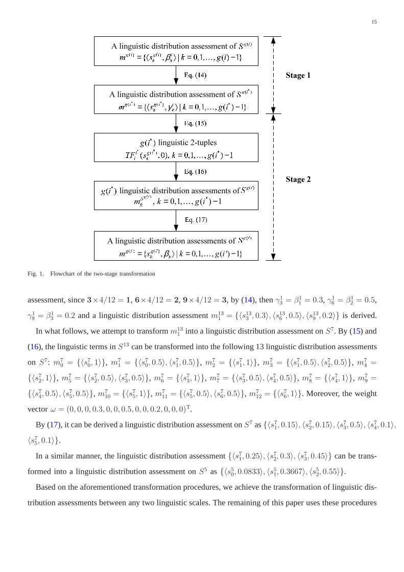
The procedures of the two-stage transformation are illustrated by Fig.1.
Theorem 3. mg(i′) derived by Definition13 is a linguistic distribution assessment.
Proof: Based on the above analysis, we have that eachmg(i′), k = 0, 1, . . . , g(i∗)− 1 is a linguistic
distribution assessment. Moreover,∑g(i∗)−1
k=0 γik = 1. Since the weighted average of some linguistic
distribution assessments is also a linguistic distribution assessment [26], mg(i′) is a linguistic distribution
assessment.
Example 4. Let S5 = s50, s51, . . . , s
54 andS7 = s70, s
71, . . . , s
76 be two linguistic term sets, and there are
two linguistic distribution assessments to be fused, i.e.〈s51, 0.3〉, 〈s52, 0.5〉, 〈s
53, 0.2〉 and〈s71, 0.25〉, 〈s
72, 0.3〉,
〈s73, 0.45〉.
Here, there are two linguistic term sets, i.e.S5 andS7. According to Proposition1, we haveg(i∗) =
LCM(4, 6) = 12. Therefore,Sg(i∗) = S13 = s130 , s131 , . . . , s1312. For the first linguistic distribution
15
β= = … −
!"
#$% &'()
*+, -./0
123 4567
89: ;<=>
?@ AB CD
E FG H I J KL M N OPQR S T U VW
X Y Z [ \] ^_ ` a b cγ= d e = … −
fg hi j
k lm n op qrst uvwx y z |
~ = … −
= … −
¡ ¢£ ¤ ¥¦ § ¨ © ª« ¬ β= ⟩ = … −
Fig. 1. Flowchart of the two-stage transformation
assessment, since3×4/12 = 1, 6×4/12 = 2, 9×4/12 = 3, by (14), thenγ13 = β1
1 = 0.3, γ16 = β1
2 = 0.5,
γ19 = β1
3 = 0.2 and a linguistic distribution assessmentm131 = 〈s133 , 0.3〉, 〈s136 , 0.5〉, 〈s139 , 0.2〉 is derived.
In what follows, we attempt to transformm131 into a linguistic distribution assessment onS7. By (15) and
(16), the linguistic terms inS13 can be transformed into the following 13 linguistic distribution assessments
on S7: m70 = 〈s70, 1〉, m7
1 = 〈s70, 0.5〉, 〈s71, 0.5〉, m7
2 = 〈s71, 1〉, m73 = 〈s71, 0.5〉, 〈s
72, 0.5〉, m7
4 =
〈s72, 1〉, m75 = 〈s72, 0.5〉, 〈s
73, 0.5〉, m7
6 = 〈s73, 1〉, m77 = 〈s73, 0.5〉, 〈s
74, 0.5〉, m7
8 = 〈s74, 1〉, m79 =
〈s74, 0.5〉, 〈s75, 0.5〉, m7
10 = 〈s75, 1〉, m711 = 〈s75, 0.5〉, 〈s
76, 0.5〉, m7
12 = 〈s76, 1〉. Moreover, the weight
vectorω = (0, 0, 0, 0.3, 0, 0, 0.5, 0, 0, 0.2, 0, 0, 0)T.
By (17), it can be derived a linguistic distribution assessment onS7 as〈s71, 0.15〉, 〈s72, 0.15〉, 〈s
73, 0.5〉, 〈s
74, 0.1〉,
〈s75, 0.1〉.
In a similar manner, the linguistic distribution assessment 〈s71, 0.25〉, 〈s72, 0.3〉, 〈s
73, 0.45〉 can be trans-
formed into a linguistic distribution assessment onS5 as〈s50, 0.0833〉, 〈s51, 0.3667〉, 〈s
52, 0.55〉.
Based on the aforementioned transformation procedures, weachieve the transformation of linguistic dis-
tribution assessments between any two linguistic scales. The remaining of this paper uses these procedures

16
to solve large-scale MAGDM problems with multi-granular linguistic information.
V. LARGE-SCALE LINGUISTIC MAGDM BASED ON MULTI-GRANULAR LINGUISTIC DISTRIBUTION
ASSESSMENTS
In this section, an approach for linguistic large-scale MAGDM based on multi-granular linguistic
distribution assessments is presented, which is suitable to deal with LGDM problems. The first novelty of
the proposed approach is the use of linguistic distributionassessments to represent the assessments of the
group, which keeps the maximum information elicited by decision makers of the group in initial stages
of the decision process. Another novelty is that the proposed approach allows the use of multi-granular
linguistic information, which provides a flexible way for decision makers with different background and
knowledge to express their assessment information. First of all, the formulation of the linguistic large-scale
MAGDM problem is introduced.
A. Formulation of the large-scale linguistic MAGDM problem
For the convenience of description, letI = 1, 2, . . . , n, J = 1, 2, . . . , m, L = 1, 2, . . . , q andH =
1, 2, . . . , r. Consider the following linguistic large-scale MAGDM problem. LetG = G1, G2, . . . , Gn
be a finite set of alternatives,C = C1, C2, . . . , Cm be the set of attributes,D = d1, d2, . . . , dq be the
set of a large group of decision makers. The weighting vectorof the attributes isw = (w1, w2, . . . , wm)T,
where0 6 wj 6 1, j ∈ J,m∑
j=1
wj = 1. In the decision making process, the decision makers provide their
assessments for each alternative with respect to each attribute using linguistic terms.
To make it more convenient for decision makers to express their assessments over alternatives, multi-
granular linguistic term sets are allowed in our MAGDM problem. Let S = Sg(1), Sg(2), . . . , Sg(r)
be the linguistic term sets to be used by the decision makers,whereSg(h) = sg(h)0 , s
g(h)1 , . . . , s
g(h)g(h)−1
is a linguistic term set with a granularity ofSg(h), h ∈ H. During the decision process, each decision
maker elicits his/her linguistic preferences in only one linguistic term set for his/her assessments. The more
knowledge has the decision maker about the problem the more granularity. Conversely, the less knowledge
the less granularity. Therefore, the set of decision makerscan be divided intor groups according to the
linguistic term sets used. For convenience, letD = D1, D2, . . . , Dr, whereDh is the set of decision
makers who select the linguistic term setSg(h), h ∈ H. Moreover, the assessment of theith alternative
with respect to thejth attribute provided by thelth decision maker is denoted byxlij , thenxl
ij ∈ Sg(h),
i ∈ I, j ∈ J , dl ∈ Dh, h ∈ H. The decision makers assessments are summarized in TableI. The GDM

17
TABLE IDECISION INFORMATION OF THE DECISION MAKERS
AlternativesAttributes
C1 C2 . . . Cm
G1 x111 . . . xq
11 x112 . . . xq
12 . . . x11m . . . xq
1m
G2 x121 . . . xq
21 x122 . . . xq
22 . . . x12m . . . xq
2m
. . . . . . . . . . . . . . .
Gn x1n1 . . . xq
n1 x1n2 . . . xq
n2 . . . x1nm . . . xq
nm
problem must obtain a solution of the best alternative through fusing the information provided by the
decision makers.
B. The proposed MAGDM approach
Here, it is proposed an approach for solving MAGDM problems dealing with multi-granular linguistic
information modeled by linguistic distribution assessments. This decision process applies a multi-step
aggregation method to the linguistic distribution assessments, by unifying them. Subsequently the weights
of the attributes are determined for aggregating the attribute values and ranking the alternatives, eventually
the collective assessments are represented in an easy understanding way. These steps are further detailed
below.
1) Representing decision makers’ assessments by linguistic distribution assessments:To keep the
maximum information elicited by decision makers of the group in initial stages of the decision process,
it is used linguistic distribution assessments to represent the linguistic information. As multi-granular
linguistic distribution assessments are elicited by different decision makers, firstly collective assessments
over each alternative with respect to each attribute assessed in the same linguistic term set are computed.
Let zhij = 〈sg(h)k , βh
ij,k〉|k = 0, 1, . . . , g(h)− 1 denote the linguistic distribution assessment on theith
alternative with respect to thejth attribute from the decision makers using the linguistic term setSg(h),
i ∈ I, j ∈ J , h ∈ H, then the following two cases are considered.
a) The decision makers are of equal importance.In this case,
βhij,k =
#l|xlij = s
g(h)k , l ∈ L
#Dh
, i ∈ I, j ∈ J, k = 0, 1, . . . , g(h)− 1, h ∈ H. (18)
where#(·) is the cardinality of the set.

18
Accordingly, the weight of the decision makers who utilize the linguistic term setSg(h) is obtained as
ωh = #Dh/q, h ∈ H.
b) The decision makers are of unequal importance.Let λ = (λ1, λ2, . . . , λq)T be the weighting
vector of the decision makers, where0 6 λl 6 1, l ∈ L,q∑
l=1
λl = 1, then we have
βhij,k =
∑
l∈P kijλl
∑
dl∈Dhλl
, (19)
whereP hij,k = l|xl
ij = sg(h)k , l ∈ L, i ∈ I, j ∈ J , k = 0, 1, . . . , g(h)− 1, h ∈ H.
Similarly, the weight of the decision makers who utilize thelinguistic term setSg(h) is obtained as
ωh =∑
dl∈Dhλl, h ∈ H.
It is easy to verify thatzhij derived by (18) and (19) are linguistic distribution assessments onSg(h),
i ∈ I, j ∈ J , h ∈ H. A simple example to demonstrate this step is described below.
Example 5. Assume that five decision makers want to evaluate a new product by considering three
attributes, including safety, cost and technical performance. The first two decision makers provide his
linguistic assessments over the product using a linguisticterm setS5 = s50, s51, . . . , s
54 and the other
three decision makers use a linguistic term setS7 = s70, s71, . . . , s
76, as demonstrated in TableII .
TABLE IIASSESSMENTS OF THE NEW PRODUCT
AlternativesAttributes
C1: Safety C2: Cost C3: Tech. P.
G1 s54 s53 s75 s76 s76 s51 s52 s73 s73 s74 s51 s51 s73 s72 s72
Let S = S5, S7 be the set of linguistic domains. If the three decision makers are of equal importance,
thenβ111,0 = β1
11,1 = β111,2 = 0, β1
11,3 =#22
= 0.5, β111,4 = #1
2= 0.5. Hence, the collective assessment
over G1 with respect toC1 from decision makers usingS5 can be denoted by a linguistic distribution
assessmentz111 = 〈s53, 0.5〉, 〈s54, 0.5〉. In a similar manner, the collective assessment overG1 with respect
to C1 from decision makers usingS7 is denoted byz211 = 〈s75, 0.333〉, 〈s76, 0.667〉. The collective
assessments overG1 with respect to all the attributes are showed in TableIII .
If the weighting vector of the three decision makers isλ = (0.2, 0.3, 0.2, 0.15, 0.15)T, thenP 111,0 =
P 111,1 = P 1
11,2 = φ, P 111,3 = 2, P 1
11,4 = 1. It follows that β111,0 = β1
11,1 = β111,2 = 0, β1
11,3 =
λ2/(λ1 + λ2) = 0.6, β111,4 = λ1/(λ1 + λ2) = 0.4. Therefore, the the group’s assessments overG1

19
TABLE IIIL INGUISTIC DISTRIBUTION ASSESSMENTS WITH EQUAL IMPORTANCE
zhijAttributes
C1: Safety C2: Cost C3: Tech. P.
z11j 〈s53, 0.5〉, 〈s54, 0.5〉 〈s51, 0.5〉, 〈s
52, 0.5〉 〈s51, 1〉
z21j 〈s75, 0.333〉, 〈s76, 0.667〉 〈s73, 0.667〉, 〈s
74, 0.333〉 〈s72, 0.667〉, 〈s
73, 0.333〉
with respect toC1 from decision makers usingS5 can be denoted by a linguistic distribution assessment
〈s53, 0.4〉, 〈s54, 0.6〉. Similarly, the collective assessment overG1 with respect toC1 from decision makers
usingS7 is denoted byz211 = 〈s75, 0.4〉, 〈s76, 0.6〉. The collective assessments overG1 with respect to all
the attributes are showed in TableIV.
TABLE IVL INGUISTIC DISTRIBUTION ASSESSMENTS WITH UNEQUAL IMPORTANCE
zhijAttributes
C1: Safety C2: Cost C3: Tech. P.
z11j 〈s53, 0.6〉, 〈s54, 0.4〉 〈s51, 0.4〉, 〈s
52, 0.6〉 〈s51, 1〉
z21j 〈s75, 0.4〉, 〈s76, 0.6〉 〈s73, 0.7〉, 〈s
74, 0.3〉 〈s72, 0.6〉, 〈s
73, 0.4〉
2) Unifying the multi-granular linguistic distribution assessments:Through a transformation process,
the group’s linguistic assessments over the alternatives with respect to each attribute can be denoted asr
decision matrices, whose elements are multi-granular linguistic distribution assessments, i.e.
Zh = (zhij)n×m =
zh11 zh12 . . . zh1m
zh21 zh21 . . . z12m...
......
...
zhn1 zhn2 . . . zhnm
, h ∈ H (20)
To fuse these multi-granular linguistic distribution assessments and derive a collective opinion over
each alternative, the procedures proposed in SectionIV are utilized. The granularity of the new linguistic
term setSg(h∗) is calculated as
g(h∗) = LCM(g(1)− 1, g(2)− 1, . . . , g(r)− 1) + 1. (21)
By (12), eachzhij is transformed into a linguistic distribution assessment onSg(h∗) aszh′
ij = 〈sg(h∗)k , γh
ij,k〉|k =

20
0, 1, . . . , g(h∗)− 1, and
γhij,k =
βhij,l(h,k) if l(h, k) ∈ 0, 1, . . . , g(h)− 1;
0 if l(h, k) /∈ 0, 1, . . . , g(h)− 1,(22)
wherel(h, k) =k ∗ (g(h)− 1)
g(j∗)− 1, h ∈ H, k = 0, 1, . . . , g(h∗)− 1.
3) Aggregating the unified decision matrices:Now, all the elements of ther decision matrices are
transformed into linguistic distribution assessments over the linguistic term setSg(h∗). By applying the
DAWA operator, the collective assessments of the group on each alternative with respect to each attribute
can be calculated, which are also linguistic distribution assessments.
Let zij = 〈sg(h∗)k , γij,k〉|k = 0, 1, . . . , g(h∗)− 1 denote the collective assessment on theith alternative
with respect to thejth attribute, then
γij,k =r∑
h=1
ωhγhij,k, i ∈ I, j ∈ J, k = 0, 1, . . . , g(h∗)− 1, (23)
whereωh is the weight of the decision makers who select the linguistic term setSg(h), h ∈ H.
4) Determining the weights of the attributes:Once the collective opinions with alternatives have been
obtained, a collective decision matrix must be computed. Itis then necessary to aggregate the attribute
values to obtain the collective assessment of each alternative. Before the aggregation process, the weight
of the attributes should be determined. In this paper, the maximum deviation approach [51] is used to
determine the weights in case they are not known as a priori.
The basic idea of the maximum deviation approach [51], [52] consists of if an attribute makes the
collective values among all the alternatives have obvious differences, then it plays an important role in
choosing the best alternative. From the view of ranking alternatives, an attribute which has similar attribute
values among alternatives should be assigned a small weight; otherwise, the attribute which has larger
deviations among attribute values should be given a higher weight. Based on this idea, it is developed
an approach to determine the weights of the attributes for decision making with linguistic distribution
assessments.
By the DAWA operator, the collective assessment of each alternative can be denoted byzi = 〈sg(i∗)k , γi,k〉|
k = 0, 1, . . . , g(h∗)− 1, where
γi,k =m∑
j=1
wjγij,k, i ∈ I, k = 0, 1, . . . , g(h∗)− 1. (24)
21
For thejth attribute, the deviation among all the alternatives is denoted by
Vj(w) =n∑
i=1
n∑
l=1
d(zi, zl) =1
g(h∗)− 1
n∑
i=1
n∑
l=1
∣
∣
∣
∣
∣
∣
g(h∗)−1∑
k=0
k(γi,k − γj,k)
∣
∣
∣
∣
∣
∣
=1
g(h∗)− 1
n∑
i=1
n∑
l=1
∣
∣
∣
∣
∣
∣
g(h∗)−1∑
k=0
k(γij,k − γlj,k)
∣
∣
∣
∣
∣
∣
wj , j ∈ J.
(25)
Therefore, the deviation among all the alternatives with respect to all the attributes is calculated
V (w) =
m∑
j=1
Vj(w) =1
g(h∗)− 1
m∑
j=1
wj
n∑
i=1
n∑
l=1
∣
∣
∣
∣
∣
∣
g(h∗)−1∑
k=0
k(γij,k − γlj,k)
∣
∣
∣
∣
∣
∣
. (26)
Based on the maximum deviation approach, the following model is established to derive the weights
of the attributes:
max V (w) =1
g(h∗)− 1
m∑
j=1
wj
n∑
i=1
n∑
l=1
∣
∣
∣
∣
∣
∣
g(h∗)−1∑
k=0
k(γij,k − γlj,k)
∣
∣
∣
∣
∣
∣
s.t.m∑
j=1
wj2 = 1
wj > 0, j ∈ J.
(M-1)
By solving the model (M-1) and normalizing the weighting vector, the weight of each attribute is
derived by
wj =
n∑
i=1
n∑
l=1
∣
∣
∣
∣
∣
g(h∗)−1∑
k=0
k(γij,k − γlj,k)
∣
∣
∣
∣
∣
m∑
j=1
n∑
i=1
n∑
l=1
∣
∣
∣
∣
∣
g(h∗)−1∑
k=0
k(γij,k − γlj,k)
∣
∣
∣
∣
∣
, j ∈ J. (27)
If the weight information of attributes is partly known (please refer to the five cases in [21], [53]), the
following optimization model is established to derive the weights of the attributes:
max V (w) =1
g(h∗)− 1
m∑
j=1
wj
n∑
i=1
n∑
l=1
∣
∣
∣
∣
∣
∣
g(h∗)−1∑
k=0
k(γij,k − γlj,k)
∣
∣
∣
∣
∣
∣
s.t.m∑
j=1
wj = 1
(w1, w2, . . . , wm) ∈ Ω
wj > 0, j ∈ J,
(M-2)

22
whereΩ is the weighting vector space constructed by the partly known weight information.
By solving the model (M-2), the weighting vector can also be obtained.
5) Aggregating the attribute values and ranking the alternatives: Once the weights of the attributes are
determined, the collective assessment of each alternativecan be calculated by aggregating the attribute
values using (24). The collective assessments are denoted byzi = 〈sg(h∗)k , γi,k〉|k = 0, 1, . . . , g(h∗)− 1,
i ∈ I.
For eachzi, the expectation values and the inaccuracy function valuesare calculated by Definitions5
and9 as
E(zi) =
g(h∗)−1∑
k=0
kγi,k, i ∈ I (28)
and
T (zi) = −
g(h∗)−1∑
k=0
γi,k log2 γi,k, i ∈ I. (29)
Based on the values ofE(zi) andT (zi), the ranking of the alternatives can be derived by Definition
10. According to the ranking, the best alternative can be obtained.
6) Representing the collective assessments:By aggregating the attribute values, the collective assess-
ment of each alternative is derived which is a linguistic distribution assessment on the linguistic term
set Sg(i∗). For such linguistic distribution assessments, it is hard for decision makers to understand the
collective assessment of each alternative, since the linguistic distribution assessments are not defined on
their initial linguistic term sets. To provide interpretable final linguistic results for decision makers, it is
necessary to transform the derived collective assessmentsinto linguistic distribution assessments using the
initial linguistic term sets. Stage 2 in subsectionIV-B is utilized to achieve this goal. By doing so, the
decision makers can clearly know the overall assessments ofthe alternatives using their own linguistic
term set as well as the proportion of each linguistic term.
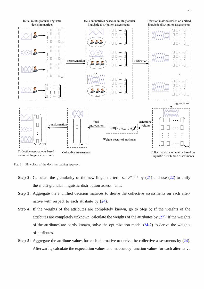
To summarize, the procedures of the proposed MAGDM approachare given below, which it is also
depicted in Fig.2.
Step 1: Gather the decision makers’ assessments and represent the assessments from the decision
makers who select the same linguistic term set using linguistic distribution assessments by
(18) or (19). In this way,r decision matrices are derived by (20). Also, determine the weights
of each decision matrix asω = (ω1, ω2, . . . , ωr)T.
23
®×
¯ °± ²³ ´µ ¶· ¸¹ º» ¼
L
L
M M M M
L
½ ¾×
¿ ÀÁ ÂÃ ÄÅ ÆÇ ÈÉ ÊË Ì
L
L
M M M M
L
Í Î×
Ï ÐÑ ÒÓ ÔÕ Ö× ØÙ ÚÛ Ü
L
L
M M M M
L
Ý Þ×
ß àá âã äå æç èé êë ì
L
L
M M M M
L
í î×
ï ðñ òó ôõ ö÷ øù úû ü
L
L
M M M M
L
ý þ×
ÿ
L
L
M M M M
L
×
L
L
M M M M
L
×
! "# $% &' () *+ ,
L
L
M M M M
L
- .×
/ 01 23 45 67 89 :; <
L
L
M M M M
L
= >×
? @A BC DE FG HI JK L
L
L
M M M M
L
M N×
L
L
M M M M
L
OP Q R = K
ST×
M
×
M
Fig. 2. Flowchart of the decision making approach
Step 2: Calculate the granularity of the new linguistic term setSg(h∗) by (21) and use (22) to unify
the multi-granular linguistic distribution assessments.
Step 3: Aggregate ther unified decision matrices to derive the collective assessments on each alter-
native with respect to each attribute by (24).
Step 4: If the weights of the attributes are completely known, go to Step 5; If the weights of the
attributes are completely unknown, calculate the weights of the attributes by (27); If the weights
of the attributes are partly known, solve the optimization model (M-2) to derive the weights
of attributes.
Step 5: Aggregate the attribute values for each alternative to derive the collective assessments by (24).
Afterwards, calculate the expectation values and inaccuracy function values for each alternative

24
and output the ranking of the alternatives by Definition10.
Step 6: If the decision makers want to know the collective assessment using the initial linguistic term
sets, represent the collective assessments of each alternative using the initial linguistic term
sets by Stage 2 in subsectionIV-B.
VI. A N ILLUSTRATIVE EXAMPLE
In this section, an example for talent recruitment is used todemonstrate the proposed MAGDM
approach. A university in China was intended to recruit a dean for the School of Business. The recruitment
process was as follows. First, the university released an opening recruitment announcement on the website.
Any people who satisfied the basic recruitment conditions could apply for the position using the online
application system before the deadline. After receiving applications from candidates at home and abroad,
the staffs of the personnel department made a strict selection by checking the application documents.
Finally, four candidates (G1, G2, G3, G4) entered the interview for further selection. To make the final
selection as fair as possible, a committee which was composed of 24 members from the academic board
of the university was established. After making face-to-face interviews with the four candidates, each
committee member was asked to provide their assessments over the four candidates with respect to
the following four criteria:C1: Academic background and influence;C2: Leadership;C3: Research and
teaching experiences;C4: International exchange and cooperation.
To facilitate the evaluation process, the committee members were allowed to provide their assessments
using multi-granular linguistic term sets, i.e. each committee member could select a linguistic term set
for assessment according to his/her interest. The linguistic term sets used were the following ones:
Sg(1) = S5 = s50 : poor, s51 : slightly poor, s52 : fair, s53 : slightly good, s54 : good; Sg(2) = S7 =
s70 : very poor, s71 : poor, s72 : slightly poor, s73 : fair, s54 : slightly good, s75 : good, s76 : very good; Sg(3) =
S9 = s90 : extremely poor, s91 : very poor, s92 : poor, s93 : slightly poor, s94 : fair, s95 : slightly good, s96 :
good, s97 : very good, s98 : extremely good.
Finally, the number of the committee members who selectedS5, S7 andS9 for assessment were 10,
8 and 6, respectively. The proposed MAGDM approach is then employed to select the most appropriate
candidate.
Step 1: After gathering the committee members’ multi-granular linguistic assessment, we conduct the
initial fusion of information and represent the collectiveassessment over each candidate with respect to
each criteria from the committee members who select the samelinguistic term set using multi-granular
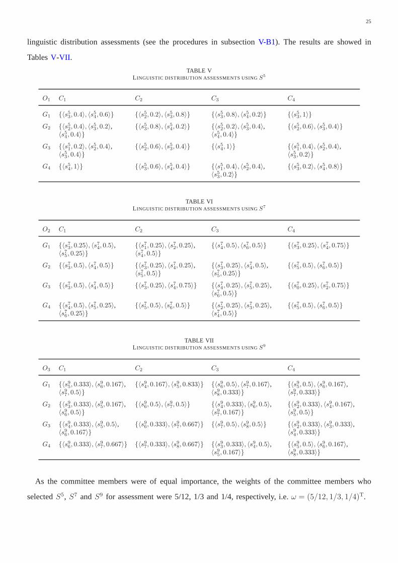
25
linguistic distribution assessments (see the procedures in subsectionV-B1). The results are showed in
TablesV-VII .
TABLE VL INGUISTIC DISTRIBUTION ASSESSMENTS USINGS5
O1 C1 C2 C3 C4
G1 〈s53, 0.4〉, 〈s5
4, 0.6〉 〈s52, 0.2〉, 〈s5
3, 0.8〉 〈s53, 0.8〉, 〈s5
4, 0.2〉 〈s53, 1〉
G2 〈s52, 0.4〉, 〈s5
3, 0.2〉,
〈s54, 0.4〉〈s5
3, 0.8〉, 〈s5
4, 0.2〉 〈s5
2, 0.2〉, 〈s5
3, 0.4〉,
〈s54, 0.4〉〈s5
2, 0.6〉, 〈s5
3, 0.4〉
G3 〈s51, 0.2〉, 〈s5
2, 0.4〉,
〈s53, 0.4〉〈s5
2, 0.6〉, 〈s5
3, 0.4〉 〈s5
4, 1〉 〈s5
1, 0.4〉, 〈s5
2, 0.4〉,
〈s53, 0.2〉
G4 〈s54, 1〉 〈s5
3, 0.6〉, 〈s5
4, 0.4〉 〈s5
1, 0.4〉, 〈s5
2, 0.4〉,
〈s53, 0.2〉〈s5
3, 0.2〉, 〈s5
4, 0.8〉
TABLE VIL INGUISTIC DISTRIBUTION ASSESSMENTS USINGS7
O2 C1 C2 C3 C4
G1 〈s73, 0.25〉, 〈s7
4, 0.5〉,
〈s75, 0.25〉〈s7
1, 0.25〉, 〈s7
2, 0.25〉,
〈s74, 0.5〉〈s7
4, 0.5〉, 〈s7
6, 0.5〉 〈s7
3, 0.25〉, 〈s7
4, 0.75〉
G2 〈s73, 0.5〉, 〈s7
4, 0.5〉 〈s7
3, 0.25〉, 〈s7
4, 0.25〉,
〈s75, 0.5〉〈s7
3, 0.25〉, 〈s7
4, 0.5〉,
〈s75, 0.25〉〈s7
5, 0.5〉, 〈s7
6, 0.5〉
G3 〈s73, 0.5〉, 〈s7
4, 0.5〉 〈s7
3, 0.25〉, 〈s7
4, 0.75〉 〈s7
4, 0.25〉, 〈s7
5, 0.25〉,
〈s76, 0.5〉〈s7
0, 0.25〉, 〈s7
2, 0.75〉
G4 〈s74, 0.5〉, 〈s7
5, 0.25〉,
〈s76, 0.25〉
〈s75, 0.5〉, 〈s7
6, 0.5〉 〈s7
2, 0.25〉, 〈s7
3, 0.25〉,
〈s74, 0.5〉
〈s75, 0.5〉, 〈s7
6, 0.5〉
TABLE VIIL INGUISTIC DISTRIBUTION ASSESSMENTS USINGS9
O3 C1 C2 C3 C4
G1 〈s95, 0.333〉, 〈s9
6, 0.167〉,
〈s97, 0.5〉〈s9
4, 0.167〉, 〈s9
5, 0.833〉 〈s9
6, 0.5〉, 〈s9
7, 0.167〉,
〈s98, 0.333〉〈s9
5, 0.5〉, 〈s9
6, 0.167〉,
〈s97, 0.333〉
G2 〈s93, 0.333〉, 〈s9
5, 0.167〉,
〈s96, 0.5〉〈s9
6, 0.5〉, 〈s9
7, 0.5〉 〈s9
4, 0.333〉, 〈s9
6, 0.5〉,
〈s97, 0.167〉〈s9
2, 0.333〉, 〈s9
4, 0.167〉,
〈s95, 0.5〉
G3 〈s94, 0.333〉, 〈s9
5, 0.5〉,
〈s96, 0.167〉
〈s96, 0.333〉, 〈s9
7, 0.667〉 〈s9
7, 0.5〉, 〈s9
8, 0.5〉 〈s9
2, 0.333〉, 〈s9
3, 0.333〉,
〈s94, 0.333〉
G4 〈s96, 0.333〉, 〈s9
7, 0.667〉 〈s9
7, 0.333〉, 〈s9
8, 0.667〉 〈s9
3, 0.333〉, 〈s9
4, 0.5〉,
〈s95, 0.167〉
〈s95, 0.5〉, 〈s9
6, 0.167〉,
〈s98, 0.333〉
As the committee members were of equal importance, the weights of the committee members who
selectedS5, S7 andS9 for assessment were 5/12, 1/3 and 1/4, respectively, i.e.ω = (5/12, 1/3, 1/4)T.

26
Step 2: The granularity of the new linguistic term setg(h∗) is calculated. Sinceg(1) = 5, g(2) = 7,
g(3) = 9, we haveg(h∗) = LCM(4, 6, 8) + 1 = 25. By (22), the linguistic distribution assessments in
TablesV - VII are transformed into linguistic distribution assessmentson Sg(h∗), as showed in Tables
VIII - X.
TABLE VIIIINDIVIDUAL DECISION MATRIX Z
1′ = (z1′
ij )4×4
O1 C1 C2 C3 C4
G1 〈s2518, 0.4〉, 〈s25
24, 0.6〉 〈s2512, 0.2〉, 〈s25
18, 0.8〉 〈s2518, 0.8〉, 〈s25
24, 0.2〉 〈s2518, 1〉
G2 〈s2512, 0.4〉, 〈s25
18, 0.2〉,
〈s2524, 0.4〉〈s25
18, 0.8〉, 〈s25
24, 0.2〉 〈s25
12, 0.2〉, 〈s25
18, 0.4〉,
〈s2524, 0.4〉〈s25
12, 0.6〉, 〈s25
18, 0.4〉
G3 〈s256, 0.2〉, 〈s25
12, 0.4〉,
〈s2518, 0.4〉〈s25
12, 0.6〉, 〈s25
18, 0.4〉 〈s25
24, 1〉 〈s25
6, 0.4〉, 〈s25
12, 0.4〉,
〈s2518, 0.2〉
G4 〈s2524, 1〉 〈s25
18, 0.6〉, 〈s25
24, 0.4〉 〈s25
6, 0.4〉, 〈s25
12, 0.4〉,
〈s2518, 0.2〉〈s25
18, 0.2〉, 〈s25
24, 0.8〉
TABLE IXINDIVIDUAL DECISION MATRIX Z
2′ = (z2′
ij )4×4
O2 C1 C2 C3 C4
G1 〈s2512, 0.25〉, 〈s2516, 0.5〉,
〈s2520, 0.25〉
〈s254 , 0.25〉, 〈s258 , 0.25〉,〈s25
16, 0.5〉
〈s2516, 0.5〉, 〈s2524, 0.5〉 〈s2512, 0.25〉, 〈s
2516, 0.75〉
G2 〈s2512, 0.5〉, 〈s2516, 0.5〉 〈s2512, 0.25〉, 〈s
2516, 0.25〉,
〈s2520, 0.5〉
〈s2512, 0.25〉, 〈s2516, 0.5〉,
〈s2520, 0.25〉
〈s2520, 0.5〉, 〈s2524, 0.5〉
G3 〈s2512, 0.5〉, 〈s2516, 0.5〉 〈s2512, 0.25〉, 〈s
2516, 0.75〉 〈s2516, 0.25〉, 〈s
2520, 0.25〉,
〈s2524, 0.5〉
〈s250 , 0.25〉, 〈s258 , 0.75〉
G4 〈s2516, 0.5〉, 〈s2520, 0.25〉,
〈s2524, 0.25〉〈s2520, 0.5〉, 〈s
2524, 0.5〉 〈s258 , 0.25〉, 〈s2512, 0.25〉,
〈s2516, 0.5〉〈s2520, 0.5〉, 〈s
2524, 0.5〉
Step 3: The three decision matrices are aggregated using the DAWA operator with a weighting vector
ω = (5/12, 1/3, 1/4)T. The aggregated decision matrix is demonstrated in TableXI .
Step 4:As the weights of the criteria are unknown, we use (27) to determine the weights of the criteria.
The weighting vector is derived asw = (0.2079, 0.1968, 0.2827, 0.3126)T.
Step 5: By applying the DAWA operator, the collective assessments of the four candidates (zi) are
calculated and showed in TableXII .
Afterwards, it is computed the expectation values of the four candidates’ collective assessments. For
each candidate, it is obtainedE(z1) = (s2518,−0.38), E(z2) = (s2517,−0.07), E(z3) = (s2515, 0.15), E(z4) =
(s2518, 0.70), which results in a rankingG4 ≻ G1 ≻ G2 ≻ G3. As a result, the best candidate isG4.

27
TABLE XINDIVIDUAL DECISION MATRIX Z
3′ = (z3′
ij )4×4
O3 C1 C2 C3 C4
G1 〈s2515, 0.333〉, 〈s2518, 0.167〉,
〈s2521, 0.5〉〈s2512, 0.167〉, 〈s
2515, 0.833〉 〈s2518, 0.5〉, 〈s
2521, 0.167〉,
〈s2524, 0.333〉〈s2515, 0.5〉, 〈s
2518, 0.167〉,
〈s2521, 0.333〉
G2 〈s259, 0.333〉, 〈s25
15, 0.167〉,
〈s2518, 0.5〉〈s25
18, 0.5〉, 〈s25
21, 0.5〉 〈s25
12, 0.333〉, 〈s25
18, 0.5〉,
〈s2521, 0.167〉〈s25
6, 0.333〉, 〈s25
12, 0.167〉,
〈s2515, 0.5〉
G3 〈s2512, 0.333〉, 〈s25
15, 0.5〉,
〈s2518, 0.167〉〈s25
18, 0.333〉, 〈s25
21, 0.667〉 〈s25
21, 0.5〉, 〈s25
24, 0.5〉 〈s25
6, 0.333〉, 〈s25
9, 0.333〉,
〈s2512, 0.333〉
G4 〈s2518, 0.333〉, 〈s25
21, 0.667〉 〈s25
21, 0.333〉, 〈s25
24, 0.667〉 〈s25
9, 0.333〉, 〈s25
12, 0.5〉,
〈s2515, 0.167〉〈s25
15, 0.5〉, 〈s25
18, 0.167〉,
〈s2524, 0.333〉
TABLE XICOLLECTIVE DECISION MATRIX Z = (zij)4×4
C1 C2 C3 C4
G1 〈s2512, 0.083〉, 〈s25
15, 0.083〉,
〈s2516, 0.167〉, 〈s25
18, 0.209〉,〈s25
20, 0.083〉, 〈s25
21, 0.125〉,
〈s2524, 0.25〉
〈s254, 0.083〉, 〈s25
8, 0.083〉,
〈s2512, 0.125〉, 〈s25
15, 0.209〉,〈s25
16, 0.167〉, 〈s25
18, 0.333〉
〈s2516, 0.167〉, 〈s25
18, 0.458〉,
〈s2521, 0.042〉, 〈s25
24, 0.333〉〈s25
12, 0.083〉, 〈s25
15, 0.125〉,
〈s2516, 0.25〉, 〈s25
18, 0.459〉,〈s25
21, 0.083〉
G2 〈s259, 0.083〉, 〈s25
12, 0.333〉,
〈s2515, 0.042〉, 〈s2516, 0.167〉,
〈s2518, 0.208〉, 〈s25
24, 0.167〉
〈s2512, 0.083〉, 〈s25
16, 0.083〉,
〈s2518, 0.459〉, 〈s2520, 0.167〉,
〈s2521, 0.125〉, 〈s25
24, 0.083〉
〈s2512, 0.25〉, 〈s25
16, 0.167〉,
〈s2518, 0.291〉, 〈s2520, 0.083〉,
〈s2521, 0.042〉, 〈s25
24, 0.167〉
〈s256, 0.083〉, 〈s25
12, 0.291〉,
〈s2515, 0.125〉, 〈s2518, 0.167〉,
〈s2520, 0.167〉, 〈s25
24, 0.167〉
G3 〈s256, 0.083〉, 〈s25
12, 0.417〉,
〈s2515, 0.125〉, 〈s25
16, 0.167〉,〈s25
18, 0.208〉
〈s2512, 0.333〉, 〈s25
16, 0.25〉,
〈s2518, 0.25〉, 〈s25
21, 0.167〉〈s25
16, 0.083〉, 〈s25
20, 0.083〉,
〈s2521, 0.125〉, 〈s25
24, 0.709〉〈s25
0, 0.083〉, 〈s25
6, 0.25〉,
〈s258 , 0.25〉, 〈s259 , 0.083〉,〈s25
12, 0.25〉, 〈s25
18, 0.084〉
G4 〈s2516, 0.167〉, 〈s25
18, 0.083〉,〈s25
20, 0.083〉, 〈s25
21, 0.167〉,
〈s2524, 0.5〉
〈s2518, 0.25〉, 〈s25
20, 0.167〉,〈s25
21, 0.083〉, 〈s25
24, 0.5〉
〈s256 , 0.167〉, 〈s258 , 0.083〉,〈s25
9, 0.083〉, 〈s25
12, 0.375〉,
〈s2515, 0.042〉, 〈s2516, 0.167〉,
〈s2518, 0.083〉
〈s2515, 0.125〉, 〈s25
18, 0.125〉,〈s25
20, 0.167〉, 〈s25
24, 0.583〉
TABLE XIICOLLECTIVE ASSESSMENTS OF THE FOUR CANDIDATES
Gi Collective assessments
G1 〈s254, 0.016〉, 〈s25
8, 0.016〉, 〈s25
12, 0.068〉, 〈s25
15, 0.098〉, 〈s25
16, 0.193〉, 〈s25
18, 0.382〉, 〈s25
20, 0.017〉, 〈s25
21, 0.064〉,
〈s2524, 0.146〉
G2 〈s256, 0.026〉, 〈s25
9, 0.017〉, 〈s25
12, 0.248〉, 〈s25
15, 0.048〉, 〈s25
16, 0.098〉, 〈s25
18, 0.268〉, 〈s25
20, 0.109〉, 〈s25
21, 0.036〉,
〈s2524, 0.150〉
G3 〈s250, 0.026〉, 〈s25
6, 0.096〉, 〈s25
8, 0.078〉, 〈s25
9, 0.026〉, 〈s25
12, 0.230〉, 〈s25
15, 0.026〉, 〈s25
16, 0.107〉, 〈s25
18, 0.119〉,
〈s2520, 0.024〉, 〈s2521, 0.068〉, 〈s
2524, 0.200〉
G4 〈s256, 0.047〉, 〈s25
8, 0.024〉, 〈s25
9, 0.023〉, 〈s25
12, 0.106〉, 〈s25
15, 0.051〉, 〈s25
16, 0.082〉, 〈s25
18, 0.129〉, 〈s25
20, 0.102〉,
〈s2521, 0.051〉, 〈s2524, 0.385〉

28
Step 6: The committee members want to know the collective assessments of each candidate, so the
procedures of Stage 2 in subsection IV-B are used to transform each zi into linguistic distribution
assessments of the initial linguistic term sets. The results are demonstrated in TablesXIII -XV. From
TablesXIII - XV, we can obverse the collective assessments of the candidates. For instance, from Table
XIII we can find that the collective assessment ofG2 is mainly abouts52 and s53, while G4 is abouts53
ands54. Besides, we can also obtain the proportion distribution ofthe linguistic terms, which reflects the
tendencies of the assessments. Therefore, the use of linguistic distribution assessments can provide more
information about the assessments over alternatives.
TABLE XIIICOLLECTIVE ASSESSMENTS OF THE FOUR CANDIDATES USING LINGUISTIC TERM SETS5
Gi Collective assessments
G1 〈s50, 0.006〉, 〈s5
1, 0.022〉, 〈s5
2, 0.186〉, 〈s5
3, 0.602〉, 〈s5
4, 0.184〉
G2 〈s51, 0.035〉, 〈s5
2, 0.313〉, 〈s5
3, 0.448〉, 〈s5
4, 0.204〉
G3 〈s50, 0.026〉, 〈s51, 0.161〉, 〈s
52, 0.318〉, 〈s
53, 0.253〉, 〈s
54, 0.242〉
G4 〈s51, 0.075〉, 〈s5
2, 0.178〉, 〈s5
3, 0.303〉, 〈s5
4, 0.444〉
TABLE XIVCOLLECTIVE ASSESSMENTS OF THE FOUR CANDIDATES USING LINGUISTIC TERM SETS7
Gi Collective assessments
G1 〈s71, 0.016〉, 〈s7
2, 0.017〉, 〈s7
3, 0.092〉, 〈s7
4, 0.457〉, 〈s7
5, 0.256〉, 〈s7
6, 0.162〉
G2 〈s71, 0.013〉, 〈s7
2, 0.026〉, 〈s7
3, 0.264〉, 〈s7
4, 0.268〉, 〈s7
5, 0.270〉, 〈s7
6, 0.159〉
G3 〈s70, 0.026〉, 〈s71, 0.048〉, 〈s
72, 0.145〉, 〈s
73, 0.244〉, 〈s
74, 0.186〉, 〈s
75, 0.134〉, 〈s
76, 0.217〉
G4 〈s71, 0.024〉, 〈s7
2, 0.065〉, 〈s7
3, 0.125〉, 〈s7
4, 0.184〉, 〈s7
5, 0.205〉, 〈s7
6, 0.397〉
TABLE XVCOLLECTIVE ASSESSMENTS OF THE FOUR CANDIDATES USING LINGUISTIC TERM SETS9
Gi Collective assessments
G1 〈s91, 0.011〉, 〈s9
2, 0.011〉, 〈s9
3, 0.011〉, 〈s9
4, 0.068〉, 〈s9
5, 0.226〉, 〈s9
6, 0.452〉, 〈s9
7, 0.075〉, 〈s9
8, 0.146〉
G2 〈s92, 0.026〉, 〈s9
3, 0.017〉, 〈s9
4, 0.248〉, 〈s9
5, 0.113〉, 〈s9
6, 0.337〉, 〈s9
7, 0.109〉, 〈s9
8, 0.150〉
G3 〈s90, 0.026〉, 〈s92, 0.122〉, 〈s
93, 0.078〉, 〈s
94, 0.2370〉, 〈s
95, 0.098〉, 〈s
96, 0.162〉, 〈s
97, 0.084〉, 〈s
98, 0.200〉
G4 〈s92, 0.055〉, 〈s9
3, 0.039〉, 〈s9
4, 0.106〉, 〈s9
5, 0.105〉, 〈s9
6, 0.191〉, 〈s9
7, 0.119〉, 〈s9
8, 0.385〉

29
VII. CONCLUSIONS
In this paper, a new linguistic computational model has beendeveloped to deal with multi-granular
linguistic distribution assessments for its application to large-scale MAGDM problems with linguistic
information.
First, different distance measures and a new ranking methodare developed to improve the management
of linguistic distribution assessments.
Second, the relationship between a linguistic 2-tuple and alinguistic distribution assessment is investi-
gated. To manage multi-granular linguistic distribution assessments, a new linguistic computational model
is then developed based on the ELH model and the transformation formulae between a linguistic 2-tuple
and a linguistic distribution assessment, which not only can be used to fuse multi-granular linguistic
distribution assessments, but also can provide interpretable aggregate linguistic results to decision makers.
Third, an approach to large-scale MAGDM with multi-granular linguistic information is proposed based
on the new linguistic computational model. The proposed approach uses linguistic distribution assessments
to represent decision makers’ assessments, which keeps themaximum information elicited by decision
makers of the group in initial stages of the decision processand can provide more information about the
collective assessments over alternatives.
Our future research will study the consensus reaching process for large-scale MAGDM problems with
multi-granular linguistic information based on the developed model. Moreover, the hesitant fuzzy linguistic
term sets proposed by Rodrıguezet al. [23] have received more and more attention from scholars [24],
[25], [54]. It will also be interesting to analyze the relationship between linguistic distribution assessments
and the hesitant fuzzy linguistic term sets in the future.
REFERENCES
[1] I. Palomares, R. M. Rodrıguez, and L. Martınez, “An attitude-driven web consensus support system for heterogeneous group decision
making,” Expert Systems with Applications, vol. 40, no. 1, pp. 139–149, 2013.
[2] W. Pedrycz, P. Ekel, and R. Parreiras,Fuzzy Multicriteria Decision-Making: Models, Methods andApplications. Chichester, UK:
John Wiley & Sons, 2011.
[3] R. M. Rodrıguez, L. Martınez, and F. Herrera, “A group decision making model dealing with comparative linguistic expressions based
on hesitant fuzzy linguistic term sets,”Information Sciences, vol. 241, pp. 28–42, 2013.
[4] M. Delgado, F. Herrera, E. Herrera-Viedma, and L. Martınez, “Combining numerical and linguistic information in group decision
making,” Information Sciences, vol. 107, no. 1-4, pp. 177–194, 1998.
[5] L. A. Zadeh, “Fuzzy logic = computing with words,”IEEE Transactions on Fuzzy Systems, vol. 4, no. 2, pp. 103–111, 1996.

30
[6] L. Martınez, D. Ruan, and F. Herrera, “Computing with words in decision support systems: An overview on models and applications,”
International Journal of Computational Intelligence Systems, vol. 3, no. 4, pp. 382–395, 2010.
[7] J. Lu, G. Zhang, D. Ruan, and F. Wu,Multi-Objective Group Decision Making. Methods, Softwareand Applications with Fuzzy Set
Techniques. Imperial College Press, 2007.
[8] N. Agell, M. Sanchez, F. Prats, and L. Rosello, “Ranking multi-attribute alternatives on the basis of linguistic labels in group decisions,”
Information Sciences, vol. 209, pp. 49–60, 2012.
[9] Y. Dong, G. Zhang, W. C. Hong, and S. Yu, “Linguistic computational model based on 2-tuples and intervals,”IEEE Transactions on
Fuzzy Systems, vol. 21, no. 6, pp. 1006–1018, 2013.
[10] D. Meng and Z. Pei, “On weighted unbalanced linguistic aggregation operators in group decision making,”Information Sciences, vol.
223, pp. 31–41, 2013.
[11] I. Palomares, L. Martınez, and F. Herrera, “A consensus model to detect and manage noncooperative behaviors in large-scale group
decision making,”IEEE Transactions on Fuzzy Systems, vol. 22, no. 3, pp. 516–530, 2014.
[12] S. Zahir, “Clusters in a group: Decision making in the vector space formulation of the analytic hierarchy process,”European Journal
of Operational Research, vol. 112, no. 3, pp. 620–634, 1999.
[13] Y. Wang, X. Ma, Y. Lao, and Y. Wang, “A fuzzy-based customer clustering approach with hierarchical structure for logistics network
optimization,” Expert Systems with Applications, vol. 41, no. 2, pp. 521–534, 2014.
[14] B. Liu, Y. Shen, X. Chen, Y. Chen, and X. Wang, “A partial binary tree DEA-DA cyclic classification model for decision makers in
complex multi-attribute large-group interval-valued intuitionistic fuzzy decision-making problems,”Information Fusion, vol. 18, pp.
119–130, 2014.
[15] X.-H. Xu, Z.-J. Du, and X.-H. Chen, “Consensus model formulti-criteria large-group emergency decision making considering non-
cooperative behaviors and minority opinions,”Decision Support Systems, vol. 79, pp. 150–160, 2015.
[16] Y. Liu, Z.-P. Fan, and X. Zhang, “A method for large groupdecision-making based on evaluation information providedby participators
from multiple groups,”Information Fusion, 2015.
[17] B. Liu, Y. Shen, W. Zhang, X. Chen, and X. Wang, “An interval-valued intuitionistic fuzzy principal component analysis model-based
method for complex multi-attribute large-group decision-making,” European Journal of Operational Research, vol. 245, no. 1, pp.
209–225, 2015.
[18] G. Carvalho, A. S. Vivacqua, J. M. Souza, and S. P. J. Medeiros, “Lasca: A large scale group decision support system,”Journal of
Universal Computer Science, vol. 17, no. 2, pp. 261–275, 2011.
[19] I. Palomares, L. Martınez, and F. Herrera, “MENTOR: A graphical monitoring tool of preferences evolution in large-scale group
decision making,”Knowledge-Based Systems, vol. 58, pp. 66–74, 2014.
[20] R. M. Rodrıguez and L. Martınez, “An analysis of symbolic linguistic computing models in decision making,”International Journal
of General Systems, vol. 42, no. 1, pp. 121–136, 2013.
[21] Z. Zhang and C. Guo, “A method for multi-granularity uncertain linguistic group decision making with incomplete weight information,”
Knowledge-Based Systems, vol. 26, pp. 111–119, 2012.
[22] J. Xu, Z. Wu, and Y. Zhang, “A consensus based method for multi-criteria group decision making under uncertain linguistic setting,”
Group Decision and Negotiation, vol. 23, no. 1, pp. 127–148, 2014.
[23] R. M. Rodrıguez, L. Martınez, and F. Herrera, “Hesitant fuzzy linguistic term sets for decision making,”IEEE Transactions on Fuzzy
Systems, vol. 20, no. 1, pp. 109–119, 2012.
[24] H. Liao, Z. Xu, and X.-J. Zeng, “Distance and similaritymeasures for hesitant fuzzy linguistic term sets and their application in
multi-criteria decision making,”Information Sciences, vol. 271, pp. 125–142, 2014.

31
[25] H. Liu and R. M. Rodrıguez, “A fuzzy envelope for hesitant fuzzy linguistic term set and its application to multicriteria decision
making,” Information Sciences, vol. 258, pp. 220–238, 2014.
[26] G. Zhang, Y. Dong, and Y. Xu, “Consistency and consensusmeasures for linguistic preference relations based on distribution
assessments,”Information Fusion, vol. 17, pp. 46–55, 2014.
[27] Y. Dong, Y. Wu, H. Zhang, and G. Zhang, “Multi-granular unbalanced linguistic distribution assessments with interval symbolic
proportions,”Knowledge-Based Systems, vol. 82, pp. 139–151, 2015.
[28] J. A. Morente-Molinera, I. J. Perez, M. R. Urena, and E. Herrera-Viedma, “On multi-granular fuzzy linguistic modeling in group
decision making problems: A systematic review and future trends,”Knowledge-Based Systems, vol. 74, pp. 49–60, 2015.
[29] F. Herrera, E. Herrera-Viedma, and L. Martınez, “A fusion approach for managing multi-granularity linguistic term sets in decision
making,” Fuzzy Sets and Systems, vol. 114, no. 1, pp. 43–58, 2000.
[30] F. Herrera and L. Martınez, “A model based on linguistic 2-tuples for dealing with multigranular hierarchical linguistic contexts in
multi-expert decision-making,”IEEE Transactions on Systems, Man, and Cybernetics, Part B:Cybernetics, vol. 31, no. 2, pp. 227–234,
2001.
[31] V. N. Huynh and Y. Nakamori, “A satisfactory-oriented approach to multiexpert decision-making with linguistic assessments,”IEEE
Transactions on Systems, Man, and Cybernetics, Part B: Cybernetics, vol. 35, no. 2, pp. 184–196, 2005.
[32] Z. Chen and D. Ben-Arieh, “On the fusion of multi-granularity linguistic label sets in group decision making,”Computers & Industrial
Engineering, vol. 51, no. 3, pp. 526–541, 2006.
[33] M. Espinilla, J. Liu, and L. Martınez, “An extended hierarchical linguistic model for decision-making problems,” Computational
Intelligence, vol. 27, no. 3, pp. 489–512, 2011.
[34] Z.-P. Fan and Y. Liu, “A method for group decision-making based on multi-granularity uncertain linguistic information,” Expert Systems
with Applications, vol. 37, no. 5, pp. 4000–4008, 2010.
[35] Y. Dong, C.-C. Li, Y. Xu, and X. Gu, “Consensus-based group decision making under multi-granular unbalanced 2-tuple linguistic
preference relations,”Group Decision and Negotiation, vol. 24, no. 2, pp. 217–242, 2015.
[36] L. Martınez and F. Herrera, “An overview on the 2-tuplelinguistic model for computing with words in decision making: Extensions,
applications and challenges,”Information Sciences, vol. 207, pp. 1–18, 2012.
[37] L. A. Zadeh, “The concept of a linguistic variable and its application to approximate reasoning-I,”Information Sciences, vol. 8, no. 3,
pp. 199–249, 1975.
[38] ——, “The concept of a linguistic variable and its application to approximate reasoning-II,”Information Sciences, vol. 8, no. 4, pp.
301–357, 1975.
[39] ——, “The concept of a linguistic variable and its application to approximate reasoning-III,”Information Sciences, vol. 9, no. 1, pp.
43–80, 1975.
[40] R. R. Yager, “An approach to ordinal decision making,”International Journal of Approximate Reasoning, vol. 12, no. 3-4, pp. 237–261,
1995.
[41] F. Herrera and L. Martınez, “A 2-tuple fuzzy linguistic representation model for computing with words,”IEEE Transactions on Fuzzy
Systems, vol. 8, no. 6, pp. 746–752, 2000.
[42] R. Degani and G. Bortolan, “The problem of linguistic approximation in clinical decision making,”International Journal of Approximate
Reasoning, vol. 2, no. 2, pp. 143–162, 1988.
[43] Z. Xu, “Uncertain linguistic aggregation operators based approach to multiple attribute group decision making under uncertain linguistic
environment,”Information Sciences, vol. 168, no. 1-4, pp. 171–184, 2004.
32
[44] J. M. Mendel and H. Wu, “Type-2 fuzzistics for symmetricinterval type-2 fuzzy sets: Part 1, forward problems,”IEEE Transactions
on Fuzzy Systems, vol. 14, no. 6, pp. 781–792, 2006.
[45] J. A. Morente-Molinera, I. J. Perez, M. R. Urena, and E. Herrera-Viedma, “Creating knowledge databases for storing and sharing people
knowledge automatically using group decision making and fuzzy ontologies,”Information Sciences, vol. 328, pp. 418–434, 2016.
[46] Y.-P. Jiang, Z.-P. Fan, and J. Ma, “A method for group decision making with multi-granularity linguistic assessment information,”
Information Sciences, vol. 178, no. 4, pp. 1098–1109, 2008.
[47] Z. Xu, “An interactive approach to multiple attribute group decision making with multigranular uncertain linguistic information,”Group
Decision and Negotiation, vol. 18, no. 2, pp. 119–145, 2009.
[48] L. Rosello, M. Sanchez, N. Agell, F. Prats, and F. A. Mazaira, “Using consensus and distances between generalizedmulti-attribute
linguistic assessments for group decision-making,”Information Fusion, vol. 17, pp. 83–92, 2014.
[49] S. Massanet, J. V. Riera, J. Torrens, and E. Herrera-Viedma, “A new linguistic computational model based on discrete fuzzy numbers
for computing with words,”Information Sciences, vol. 258, pp. 277–290, 2014.
[50] T. M. Cover and J. A. Thomas,Elements of Information Theory (Second Edition). Hoboken, New Jersey: John Wiley & Sons, 2006.
[51] Y. Wang, “Using the method of maximizing deviations to make decision for multiindicies,”Systems Engineering and Electronics,
vol. 20, no. 7, pp. 24–26, 31, 1998.
[52] Z. Wu and Y. Chen, “The maximizing deviation method for group multiple attribute decision making under linguistic environment,”
Fuzzy Sets and Systems, vol. 158, no. 14, pp. 1608–1617, 2007.
[53] Y. Xu and Q. Da, “A method for multiple attribute decision making with incomplete weight information under uncertain linguistic
environment,”Knowledge-Based Systems, vol. 21, no. 8, pp. 837–841, 2008.
[54] C. Wei, Z. Ren, and R. Rodrıguez, “A hesitant fuzzy linguistic TODIM method based on a score function,”International Journal of
Computational Intelligence Systems, vol. 8, no. 4, pp. 701–712, 2015.