1 Lecture Twelve. 2 Outline Failure Time Analysis Linear Probability Model Poisson Distribution.

1

Lecture Twelve

2

Outline

• Failure Time Analysis

• Linear Probability Model

• Poisson Distribution

3

Failure Time Analysis

• Example: Duration of Expansions

• Issue: does the probability of an expansion ending depend on how long it has lasted?

• Exponential distribution: assumes the answer since the hazard rate is constant

• Weibull distribution allows a test to be performed

4

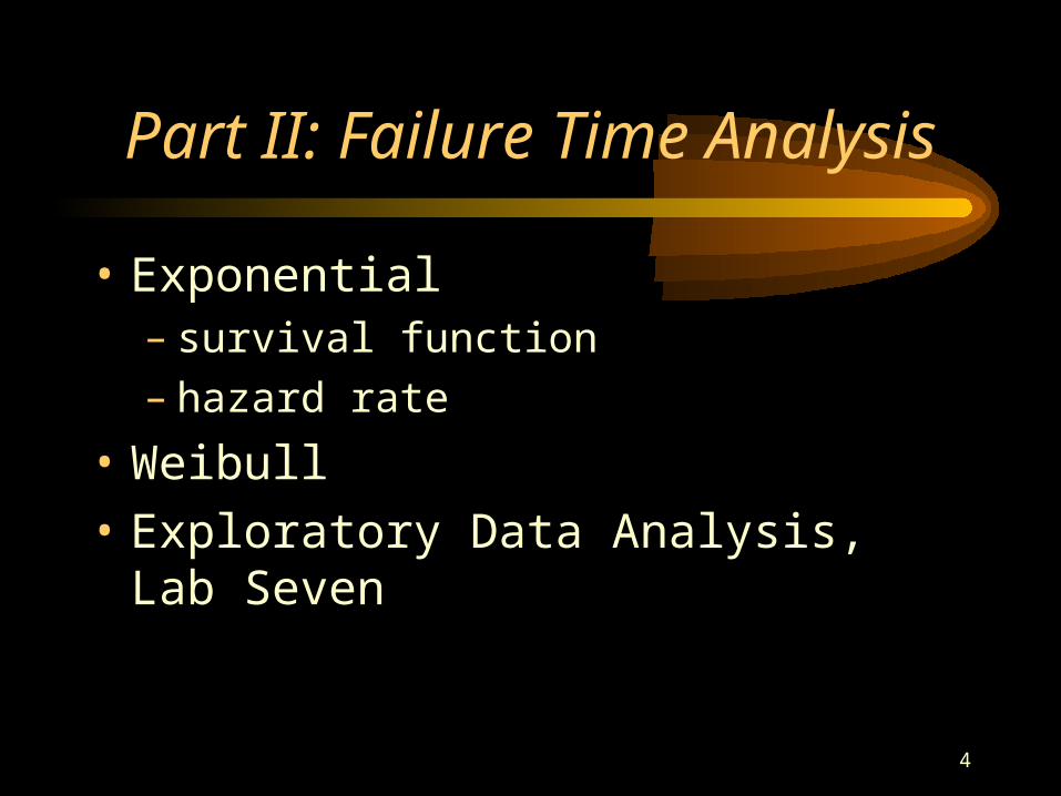
Part II: Failure Time Analysis

• Exponential– survival function– hazard rate

• Weibull

• Exploratory Data Analysis, Lab Seven

5

Duration of Post-War Economic Expansions in Months

6

Trough Peak Duration Oct. 1945 Nov. 1948 37 Oct. 1949 July 1953 45 May 1954 August 1957 39 April 1958 April 1960 24 Feb. 1961 Dec. 1969 106 Nov. 1970 Nov. 1973 36 March 1975 January 1980 58 July 1980 July 1981 12 Nov. 1982 July 1990 92 March 1991 March 2001 120

7

Estimated Survivor Function for Ten Post-War Expansions

8

Duration # Ending # At Risk F(t) Survivor0 0 10 0 112 1 10 0.1 0.924 1 9 0.2 0.836 1 8 0.3 0.737 1 7 0.4 0.639 1 6 0.5 0.545 1 5 0.6 0.458 1 4 0.7 0.392 1 3 0.8 0.2106 1 2 0.9 0.1120 1 1 1 0

9

Figure 2: Estimated Survivor Function for Post-War Expansions

0

0.2

0.4

0.6

0.8

1

1.2

0 20 40 60 80 100 120 140

Duration in Months

Su

rviv

or

Fu

nct

ion

10

Figure 3: Exponential Trendline Fitted to Estimated Survivor Function

y = 1.1972e-0.0217x

R2 = 0.9533

0

0.1

0.2

0.3

0.4

0.5

0.6

0.7

0.8

0.9

1

0 20 40 60 80 100 120

Duration in Months

Su

rviv

or

Fu

nct

ion

tetS )(

11

Figure 4: Constrained Expontial trendline, Fitted to Estimated Survivor Function

y = e-0.019x

R2 = 0.9313

0

0.1

0.2

0.3

0.4

0.5

0.6

0.7

0.8

0.9

1

0 20 40 60 80 100 120

Duration in Months

Su

rviv

or

Fu

nc

tio

n

Exponential Distribution

• Hazard rate: ratio of density function to the survivor function:

• h(t) = f(t)/S(t)

• measure of probability of failure at time t given that you have survived that long

• for the exponential it is a constant:

• h(t) = )exp(/)exp( tt

13

Duration # Ending # At Risk Inter. Haz.0 0 10 012 1 10 0.100024 1 9 0.111136 1 8 0.125037 1 7 0.142939 1 6 0.166745 1 5 0.200058 1 4 0.250092 1 3 0.3333106 1 2 0.5000120 1 1 1.0000

Interval hazard rate=#ending/#at risk

Cumulative Hazard Function

• In general:

• For the exponential,

t

duuhtH0

)()(

t

tdutH0

)(

15

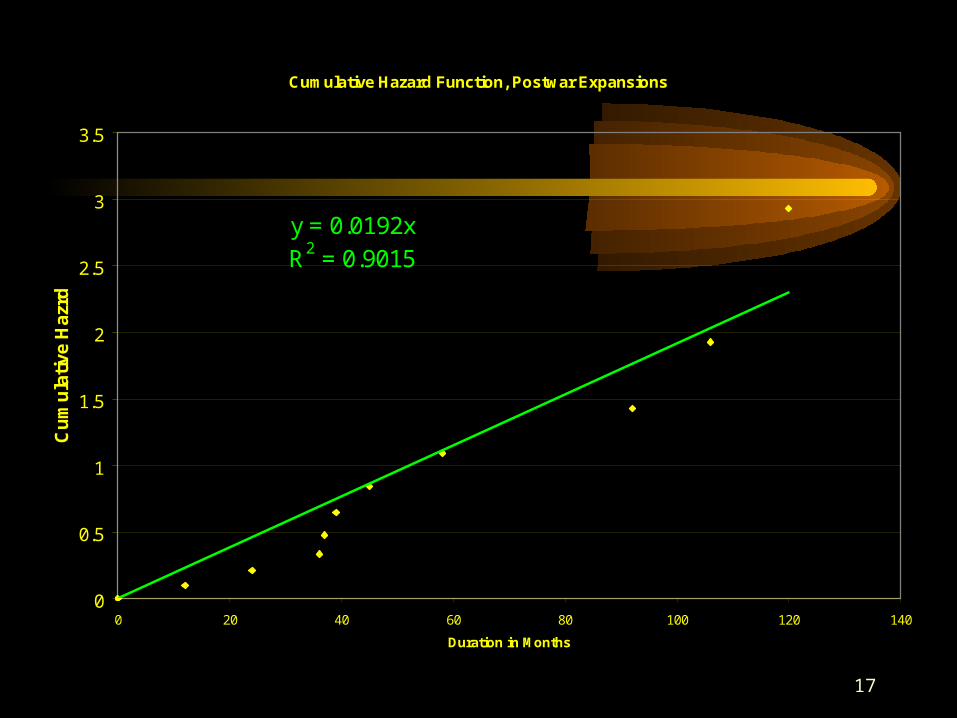
Duration # Ending # At Risk Inter. Haz.Cum. Hazard0 0 10 0 012 1 10 0.1000 0.100024 1 9 0.1111 0.211136 1 8 0.1250 0.336137 1 7 0.1429 0.479039 1 6 0.1667 0.645645 1 5 0.2000 0.845658 1 4 0.2500 1.095692 1 3 0.3333 1.4290106 1 2 0.5000 1.929120 1 1 1.0000 2.929

16

Cumulative Hazard Function: Postwar Expansions

y = 0.0223x - 0.2422R2 = 0.9288

-0.5

0

0.5

1

1.5

2

2.5

3

3.5

0 20 40 60 80 100 120 140

Duration in Months

Cu

mu

lati

ve H

azar

d

17

Cumulative Hazard Function, Postwar Expansions

y = 0.0192xR2 = 0.9015

0

0.5

1

1.5

2

2.5

3

3.5

0 20 40 60 80 100 120 140

Duration in Months

Cu

mu

lati

ve H

azrd

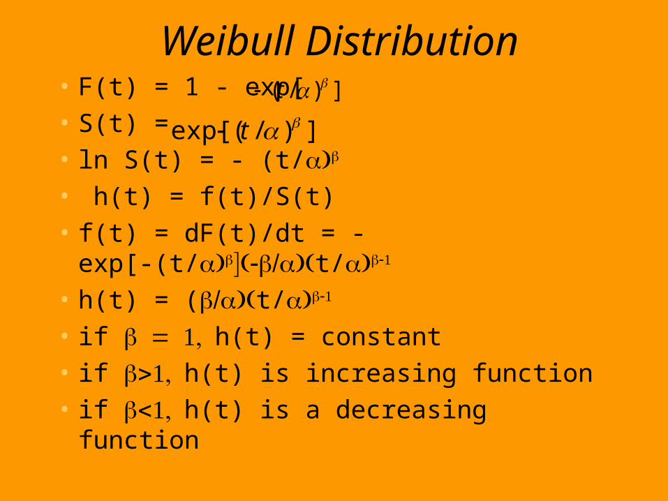
Weibull Distribution• F(t) = 1 - exp[

• S(t) =

• ln S(t) = - (t/

• h(t) = f(t)/S(t)

• f(t) = dF(t)/dt = - exp[-(t/t/

• h(t) = (t/

• if h(t) = constant

• if h(t) is increasing function

• if h(t) is a decreasing function

])/( t

])/(exp[ t

19

Weibull Distribution

• Cumulative Hazard Function

ttH

ttH

ln])/1ln[()(ln

)/1()(

20

Cumulative Hazard Function, Post-War Expansions

0.1

1

10

10 100 1000

Duration in Months

Cu

mu

lati

ve H

azar

d

21

-3

-2

-1

0

1

2

2.0 2.5 3.0 3.5 4.0 4.5 5.0

LNDUR

LNC

UM

HA

Z

Log-Log Plot of Cumulativ e Hazard Function Vs. Duration, Post-War Expansions

22

Dependent Variable: LNCUMHAZMethod: Least Squares

Sample: 2 11Included observations: 10

Variable Coefficient Std. Error t-Statistic Prob.

LNDUR 1.436662 0.103558 13.87303 0.0000C -5.920740 0.403303 -14.68061 0.0000

R-squared 0.960092 Mean dependent var -0.409591 Adjusted R-squared 0.955103 S.D. dependent var 1.038386 S.E. of regression 0.220022 Akaike info criterion -0.013326 Sum squared resid 0.387276 Schwarz criterion 0.047191 Log likelihood 2.066628 F-statistic 192.4609 Durbin-Watson stat 1.210695 Prob(F-statistic) 0.000001

23

Is Beta More Than One?

• H0: beta=1

• HAA: beta>1, and hazard rate is increasing : beta>1, and hazard rate is increasing

with time, i.e. expansions are more likely to with time, i.e. expansions are more likely to end the longer they lastend the longer they last

• t = ( 1.437 - 1)/0.104 = 4.20t = ( 1.437 - 1)/0.104 = 4.20

24

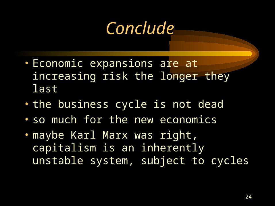
Conclude

• Economic expansions are at increasing risk the longer they last

• the business cycle is not dead

• so much for the new economics

• maybe Karl Marx was right, capitalism is an inherently unstable system, subject to cycles

25

Source:Wayne Nelson, Applied Life data Analysis(1982) John WileyDiesel Generators, hours to fan failure, (+ indicates running time, i.e. still running whenlast observed)

Hours # Ending # At Risk Interval Interval Hazard Rate Cumulative Hazard Rate450

460+11501150

1560+1600

1660+1850+1850+1850+1850+1850+2030+2030+2030+

207020702080

2200+

Lab Seven

26

Source:Wayne Nelson, Applied Life data Analysis(1982) John WileyDiesel Generators, hours to fan failure, (+ indicates running time, i.e. still running when last observed)

Hours # Ending # At Risk Interval Interval Hazard Rate Cumulative Hazard Rate450 1 70 450

460+ 681150 2 68 7001150

1560+ 651600 1 65 450

1660+ 631850+ 621850+ 611850+ 601850+ 591850+ 582030+ 572030+ 562030+ 55

2070 2 55 47020702080 1 53 10

27

Source:Wayne Nelson, Applied Life data Analysis(1982) John WileyDiesel Generators, hours to fan failure, (+ indicates running time, i.e. still running whenlast observed)

Hours # Ending # At Risk Interval Interval Hazard Rate Cumulative Hazard Rate450 1 70 450 0.0143 0.0143

460+ 681150 2 68 700 0.0294 0.04371150

1560+ 651600 1 65 450 0.0154 0.0591

1660+ 631850+ 621850+ 611850+ 601850+ 591850+ 582030+ 572030+ 562030+ 55

2070 2 55 470 0.0364 0.095520702080 1 53 10 0.0189 0.1143

2200+ 51

28

Cumulative Hazard Rate for Fan Failure

y = 4E-05x + 0.0089

R2 = 0.9816

0

0.05

0.1

0.15

0.2

0.25

0.3

0.35

0.4

0 1000 2000 3000 4000 5000 6000 7000 8000 9000 10000

Duration in Hours

Cu

mu

lati

ve H

azar

d

29

Cumulative Hazard Rate For Fan Failure

y = 4E-05x + 0.0089

R2 = 0.9816

0

0.05

0.1

0.15

0.2

0.25

0.3

0.35

0.4

0 2000 4000 6000 8000 10000

Duration in Hours

Cu

mu

lati

ve

Ha

zard

30

SUMMARY OUTPUT

Regression StatisticsMultiple R 0.990735441R Square 0.981556714Adjusted R Square 0.979251304Standard Error 0.014359467Observations 10

ANOVAdf SS MS F Significance F

Regression 1 0.087789735 0.08779 425.7622 3.19E-08Residual 8 0.001649554 0.000206Total 9 0.089439289

Coefficients Standard Error t Stat P-value Lower 95%Upper 95%Lower 95.0%Upper 95.0%Intercept 0.008850453 0.007759834 1.140547 0.287051 -0.00904 0.026745 -0.00904 0.026745X Variable 1 3.89324E-05 1.88681E-06 20.63401 3.19E-08 3.46E-05 4.33E-05 3.46E-05 4.33E-05

Lambda= 3.89 x 10-5, mean=25,707 hrs

Regress Cumulative Hazard on Duration

31

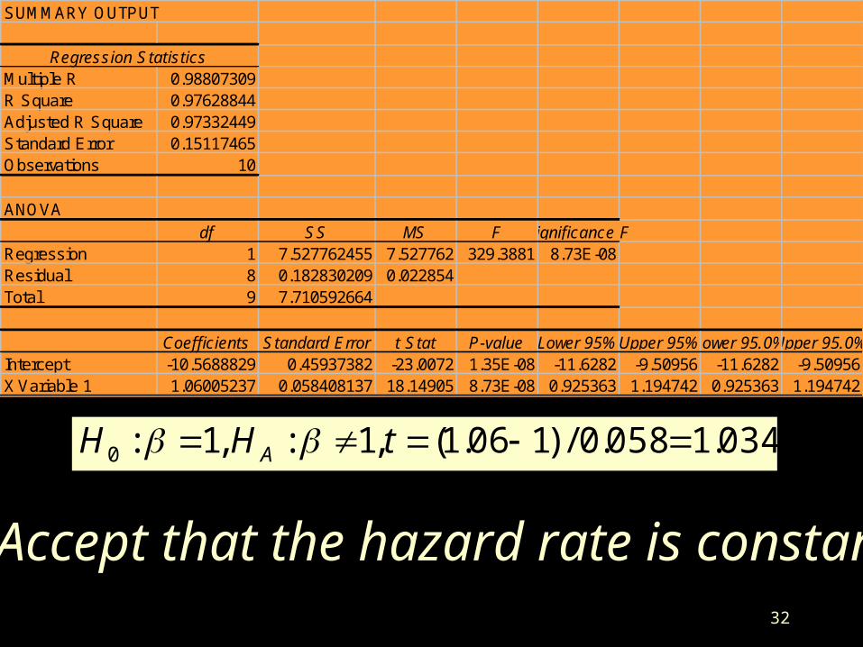
Fan Failure

• Is the hazard rate really constant?

• Regress ln cumulative hazard on ln duration

32

SUMMARY OUTPUT




Coefficients Standard Error t Stat P-value Lower 95%Upper 95%Lower 95.0%Upper 95.0%Intercept -10.5688829 0.45937382 -23.0072 1.35E-08 -11.6282 -9.50956 -11.6282 -9.50956X Variable 1 1.06005237 0.058408137 18.14905 8.73E-08 0.925363 1.194742 0.925363 1.194742

034.1058.0/)106.1(,1:,1:0 tHH A

Accept that the hazard rate is constant

33

Part II: Linear Probability Model

34

Lab Six

• Lottery

• what effect do the zeros have on the regression of % income spent on the lottery versus explanatory variables such as household income?

35

LOTTERY AGE CHILDREN EDUCATION INCOME 5.000000 50.00000 2.000000 15.00000 41.00000 7.000000 26.00000 0.000000 10.00000 22.00000 0.000000 40.00000 3.000000 13.00000 24.00000 10.00000 46.00000 2.000000 9.000000 20.00000 5.000000 40.00000 3.000000 14.00000 32.00000 5.000000 39.00000 2.000000 15.00000 42.00000 3.000000 36.00000 3.000000 8.000000 18.00000 0.000000 44.00000 1.000000 16.00000 47.00000 0.000000 47.00000 4.000000 20.00000 85.00000 6.000000 52.00000 1.000000 10.00000 23.00000 0.000000 51.00000 2.000000 18.00000 61.00000 0.000000 41.00000 2.000000 17.00000 70.00000 12.00000 42.00000 2.000000 9.000000 22.00000 7.000000 53.00000 1.000000 12.00000 27.00000 11.00000 72.00000 1.000000 9.000000 25.00000

Data

0

5

10

15

0 20 40 60 80 100

INCOME

LOT

TE

RY

OLSRegression

37

Percent of Income Spent on the Lottey

-6

-4

-2

0

2

4

6

8

10

12

14

0 20 40 60 80 100

Household Income

Pe

rce

nt

on

Lo

tte

ry

lottery

tobit fitted

Linear (lottery)

OLS slope biased toward zero

38

Effect of the Zeros on Regression

• Bias the OLS regression slope towards zero

• can’t throw away the zeros, this is the mistake the NASA engineers made with Challenger. They threw away the launches where no o-rings had failed.

• Start with a simpler model: does the household play the lottery or not?

39

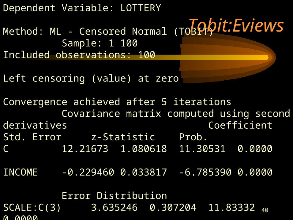
First Compare Tobit Slope to OLS Slope

• Tobit slope: -0.229

• OLS slope: -0.142

40

Dependent Variable: LOTTERYMethod: ML - Censored Normal (TOBIT)Sample: 1 100Included observations: 100Left censoring (value) at zeroConvergence achieved after 5 iterationsCovariance matrix computed using second derivatives

Coefficient Std. Error z-Statistic Prob. C 12.21673 1.080618 11.30531 0.0000INCOME -0.229460 0.033817 -6.785390 0.0000

Error DistributionSCALE:C(3) 3.635246 0.307204 11.83332 0.0000R-squared 0.365088 Mean dependent var 5.390000 Adjusted R-squared 0.351997 S.D. dependent var 3.786993 S.E. of regression 3.048478Akaike info criterion 4.621338 Sum squared resid 901.4421Schwarz criterion 4.699493 Log likelihood-228.0669 Hannan-Quinn criter. 4.652969 Avg. log likelihood -2.280669Left censored obs 23 Right censored obs 0Uncensored obs 77 Total obs 100

Tobit:Eviews

41

SUMMARY OUTPUT




Coefficients Standard Error t Stat P-value Lower 95% Upper 95%Lower 95.0%Upper 95.0%Intercept 10.076761 0.718559336 14.02356 3.6661E-25 8.65080379 11.50272 8.650804 11.50272X Variable 1 -0.142368 0.0197268 -7.21699 1.1396E-10 -0.1815154 -0.10322 -0.18152 -0.10322

OLS Excel

42

Bernoulli Variable: Bern

• Bern = 0*(lottery=0) + 1*(lottery>0)

• Linear Probability Model: dummy dependent variable

• Bern(i) = c + a*income + b*age +d*children + f*education + e(i)

43

BERN LOTTERY1 51 70 01 101 51 51 30 00 01 60 00 01 121 71 11

44

Bern age children education income

0 40.49 1.78 15.57 47.565

1 44.19 1.78 11.94 28.545

Averages for Players and Non-Players

45

0.0

0.2

0.4

0.6

0.8

1.0

0 20 40 60 80 100

INCOME

BE

RN

Linear Probability Model: Play Lottery, Yes or No

46

Dependent Variable: BERN Method: Least SquaresSample: 1 100Included observations: 100

Variable Coefficient Std. Error t-Statistic Prob.

C 1.226152 0.085229 14.38653 0.0000INCOME -0.013856 0.002340 -5.921989 0.0000

R-squared 0.263545 Mean dependent var 0.770000 Adjusted R-squared 0.256030 S.D. dependent var 0.422953 S.E. of regression 0.364812 Akaike info criterion 0.840929 Sum squared resid 13.04261 Schwarz criterion 0.893032 Log likelihood -40.04644 F-statistic 35.06996 Durbin-Watson stat 2.043370 Prob(F-statistic) 0.000000

47

Linear Probability Model

• Note: in the linear probability model, income is determining the probability of playing the lottery not the % of income spent on the lottery, so the interpretation of the slope is different.

48

-0.5

0.0

0.5

1.0

1.5

0 20 40 60 80 100

INCOME

BE

RN

HA

T

Linear Probabilty Model of Playing the Lottery Vs. Income

49

Non-Linear Probability Models

• Probit (Normit)

50

Dependent Variable: BERNMethod: ML - Binary ProbitSample: 1 100Included observations: 100Convergence achieved after 4 iterationsCovariance matrix computed using second derivatives

Variable Coefficient Std. Error z-Statistic Prob. C 2.373242 0.409671 5.793039 0.0000INCOME -0.046799 0.011017 -4.248030 0.0000

Mean dependent var 0.770000 S.D. dependent var 0.422953 S.E. of regression 0.362314 Akaike info criterion 0.876836 Sum squared resid 12.86458 Schwarz criterion 0.928939 Log likelihood-41.84178 Hannan-Quinn criter. 0.897923 Restr. log likelihood -53.92763 Avg. log likelihood -0.418418 LR statistic (1 df) 24.17171McFadden R-squared 0.224112 Probability(LR stat) 8.81E-07Obs with Dep=0 23 Total obs 100Obs with Dep=1 77

51

0.0

0.2

0.4

0.6

0.8

1.0

0 20 40 60 80 100

INCOME

PR

OB

ITH

AT

Estimated Probit Probability Model of Playing the Lottery

Part IV. Poisson Approximation to Binomial

• Conditions:

• f(x) = {exp[-] x }/x!

• Assumptions:– the number of events occurring in non-

overlapping intervals are independent– the probability of a single event occurring in a

small interval is approximately proportional to the interval

– the probability of more than one event in an interval is negligible

50,1)1(,0 npp

53

Example

• Ten % of tools produced in a manufacturing process are defective. What is the probability of finding exactly two defectives in a random sample of 10?

• Binomial: p(k=2) = 10!/(8!2!)(0.1)2(0.9)8 = 0.194

• Poisson , where the mean of the Poisson, equals n*p = 0.1 p(k=2) = {exp[-1] 12 }/2! = 0.184

1 Lecture Twelve. 2 Outline Failure Time Analysis Linear Probability Model Poisson Distribution.

Documents

Transcript of 1 Lecture Twelve. 2 Outline Failure Time Analysis Linear Probability Model Poisson Distribution.