1 Lecture 2 & 3 Linear Programming and Transportation Problem.
36
1 Lecture 2 & 3 Linear Programming and Transportation Problem
-
date post
21-Dec-2015 -
Category
Documents
-
view
227 -
download
2
Transcript of 1 Lecture 2 & 3 Linear Programming and Transportation Problem.
1
Lecture2 & 3
Linear Programmingand
Transportation Problem
2
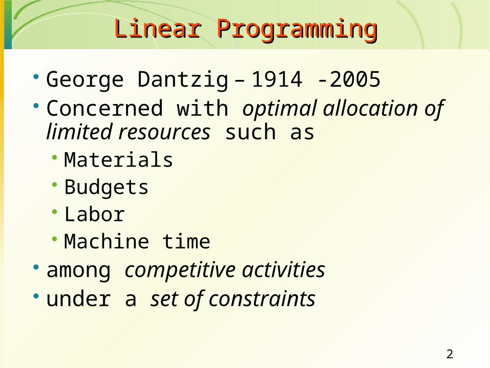
George Dantzig – 1914 -2005 Concerned with optimal allocation of limited
resources such as Materials Budgets Labor Machine time
among competitive activities under a set of constraints
Linear ProgrammingLinear Programming
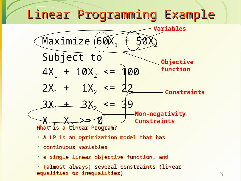
3
Maximize 60X1 + 50X2
Subject to
4X1 + 10X2 <= 100
2X1 + 1X2 <= 22
3X1 + 3X2 <= 39
X1, X2 >= 0
Linear Programming ExampleLinear Programming ExampleVariables
Objective function
Constraints
What is a Linear Program?What is a Linear Program?
• A LP is an optimization model that hasA LP is an optimization model that has
• continuous variablescontinuous variables
• a single linear objective function, anda single linear objective function, and
• (almost always) several constraints (linear equalities or inequalities)(almost always) several constraints (linear equalities or inequalities)
Non-negativity Constraints
4
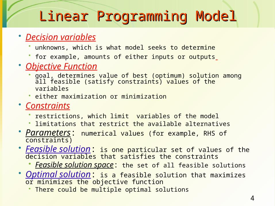
Decision variables unknowns, which is what model seeks to determine for example, amounts of either inputs or outputs
Objective Function goal, determines value of best (optimum) solution among all feasible (satisfy
constraints) values of the variables either maximization or minimization
Constraints restrictions, which limit variables of the model limitations that restrict the available alternatives
Parameters: numerical values (for example, RHS of constraints) Feasible solution: is one particular set of values of the decision variables
that satisfies the constraints Feasible solution space: the set of all feasible solutions
Optimal solution: is a feasible solution that maximizes or minimizes the objective function
There could be multiple optimal solutions
Linear Programming ModelLinear Programming Model
5
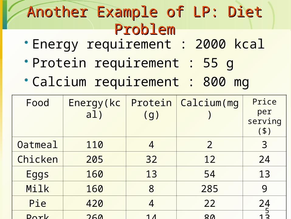
Another Example of LP: Diet Another Example of LP: Diet ProblemProblem
Energy requirement : 2000 kcal Protein requirement : 55 g Calcium requirement : 800 mg
Food Energy(kcal) Protein(g) Calcium(mg) Price per serving($)
Oatmeal 110 4 2 3
Chicken 205 32 12 24
Eggs 160 13 54 13
Milk 160 8 285 9
Pie 420 4 22 24
Pork 260 14 80 13

6
Example of LP : Diet ProblemExample of LP : Diet Problem
oatmeal: at most 4 servings/day chicken: at most 3 servings/day eggs: at most 2 servings/day milk: at most 8 servings/day pie: at most 2 servings/day pork: at most 2 servings/day
Design an optimal diet plan which minimizes the cost per
day
7
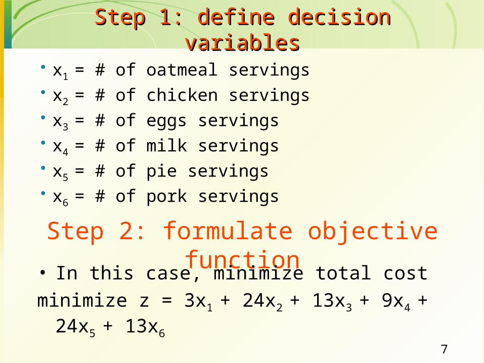
Step 1: define decision variablesStep 1: define decision variables
x1 = # of oatmeal servings x2 = # of chicken servings x3 = # of eggs servings x4 = # of milk servings x5 = # of pie servings x6 = # of pork servings
Step 2: formulate objective function• In this case, minimize total cost
minimize z = 3x1 + 24x2 + 13x3 + 9x4 + 24x5 + 13x6
8
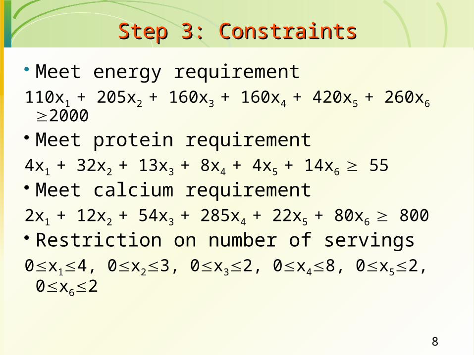
Step 3: ConstraintsStep 3: Constraints
Meet energy requirement110x1 + 205x2 + 160x3 + 160x4 + 420x5 + 260x6 2000 Meet protein requirement4x1 + 32x2 + 13x3 + 8x4 + 4x5 + 14x6 55 Meet calcium requirement2x1 + 12x2 + 54x3 + 285x4 + 22x5 + 80x6 800 Restriction on number of servings0x14, 0x23, 0x32, 0x48, 0x52, 0x62
9
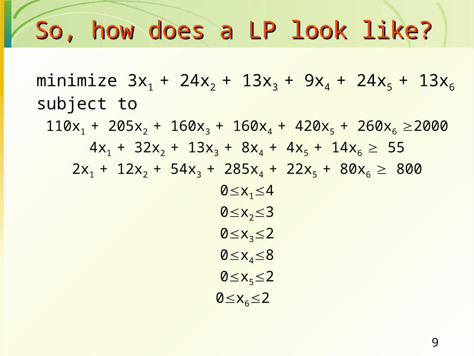
So, how does a LP look like?So, how does a LP look like?
minimize 3x1 + 24x2 + 13x3 + 9x4 + 24x5 + 13x6
subject to110x1 + 205x2 + 160x3 + 160x4 + 420x5 + 260x6 2000
4x1 + 32x2 + 13x3 + 8x4 + 4x5 + 14x6 55
2x1 + 12x2 + 54x3 + 285x4 + 22x5 + 80x6 800
0x14
0x23
0x32
0x48
0x52
0x62
10
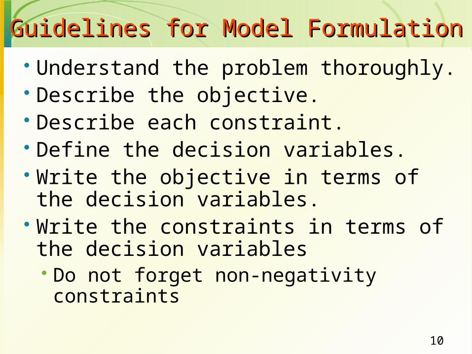
Guidelines for Model FormulationGuidelines for Model Formulation
Understand the problem thoroughly. Describe the objective. Describe each constraint. Define the decision variables. Write the objective in terms of the decision
variables. Write the constraints in terms of the decision
variables Do not forget non-negativity constraints
11
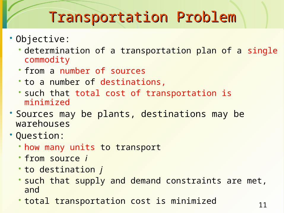
Transportation ProblemTransportation Problem Objective:
determination of a transportation plan of a single commodity from a number of sources to a number of destinations, such that total cost of transportation is minimized
Sources may be plants, destinations may be warehouses Question:
how many units to transport from source i to destination j such that supply and demand constraints are met, and total transportation cost is minimized
12
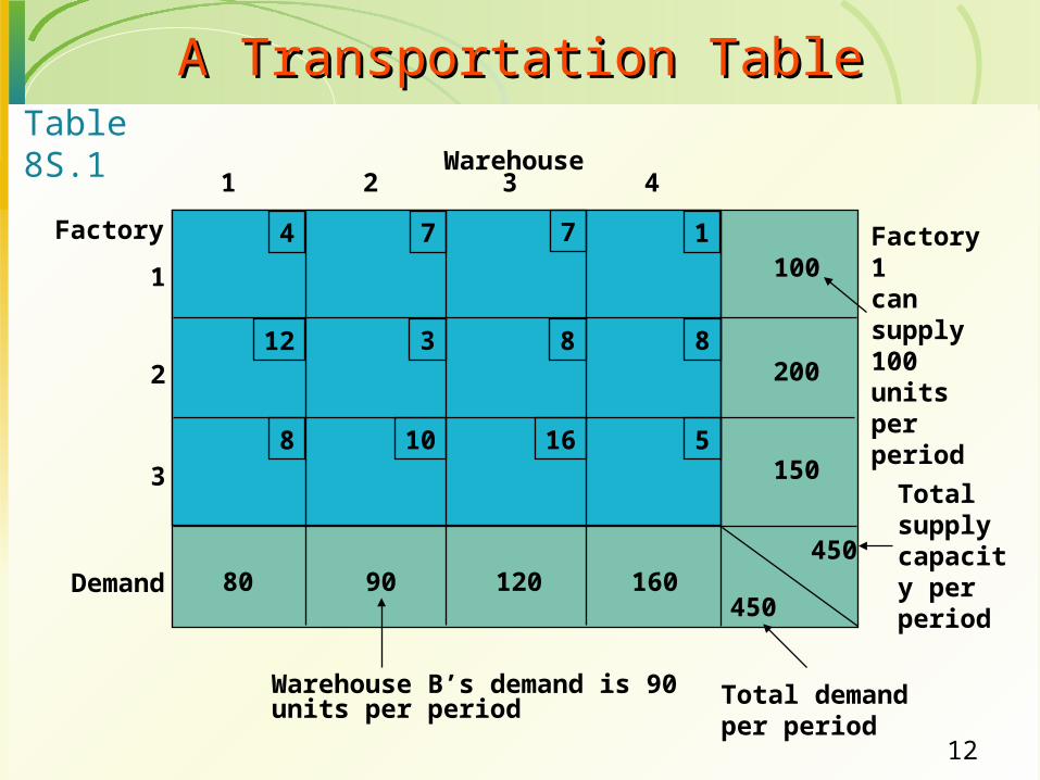
A Transportation TableA Transportation Table
Warehouse
4 7 7 1100
12 3 8 8200
8 10 16 5150
450
45080 90 120 160
1 2 3 4
1
2
3
Factory Factory 1can supply 100units per period
Demand
Table 8S.1
Warehouse B’s demand is 90 units per period Total demand
per period
Total supplycapacity perperiod
13
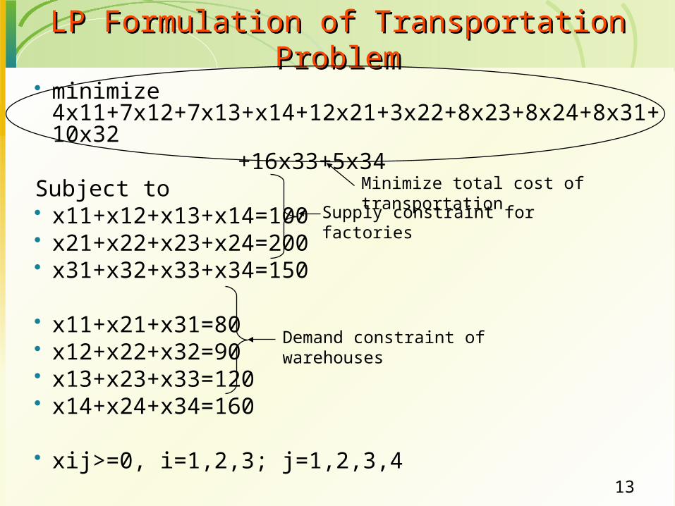
LP Formulation of Transportation ProblemLP Formulation of Transportation Problem minimize
4x11+7x12+7x13+x14+12x21+3x22+8x23+8x24+8x31+10x32 +16x33+5x34Subject to x11+x12+x13+x14=100 x21+x22+x23+x24=200 x31+x32+x33+x34=150
x11+x21+x31=80 x12+x22+x32=90 x13+x23+x33=120 x14+x24+x34=160
xij>=0, i=1,2,3; j=1,2,3,4
Supply constraint for factories
Demand constraint of warehouses
Minimize total cost of transportation
14
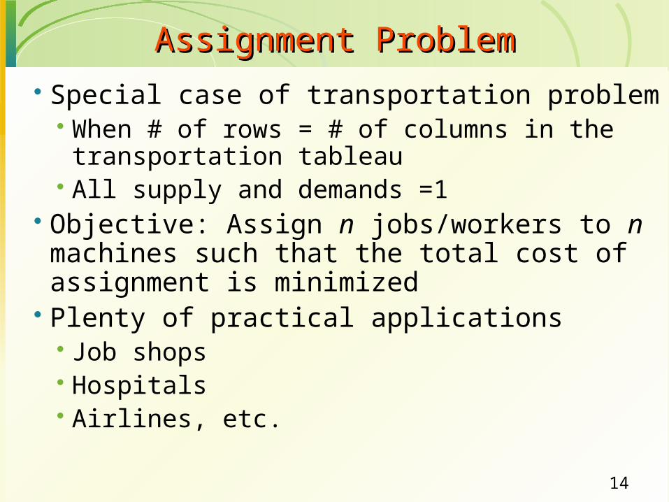
Assignment ProblemAssignment Problem
Special case of transportation problem When # of rows = # of columns in the
transportation tableau All supply and demands =1
Objective: Assign n jobs/workers to n machines such that the total cost of assignment is minimized
Plenty of practical applications Job shops Hospitals Airlines, etc.

15
Cost Table for Assignment ProblemCost Table for Assignment Problem
1 2 3 4
1 1 4 6 3
2 9 7 10 9
3 4 5 11 7
4 8 7 8 5
Worker (i)
Machine (j)
16
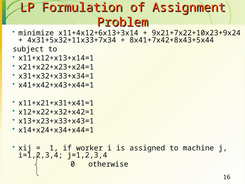
LP Formulation of Assignment ProblemLP Formulation of Assignment Problem minimize x11+4x12+6x13+3x14 + 9x21+7x22+10x23+9x24 +
4x31+5x32+11x33+7x34 + 8x41+7x42+8x43+5x44subject to x11+x12+x13+x14=1 x21+x22+x23+x24=1 x31+x32+x33+x34=1 x41+x42+x43+x44=1
x11+x21+x31+x41=1 x12+x22+x32+x42=1 x13+x23+x33+x43=1 x14+x24+x34+x44=1
xij = 1, if worker i is assigned to machine j, i=1,2,3,4; j=1,2,3,4 0 otherwise
17
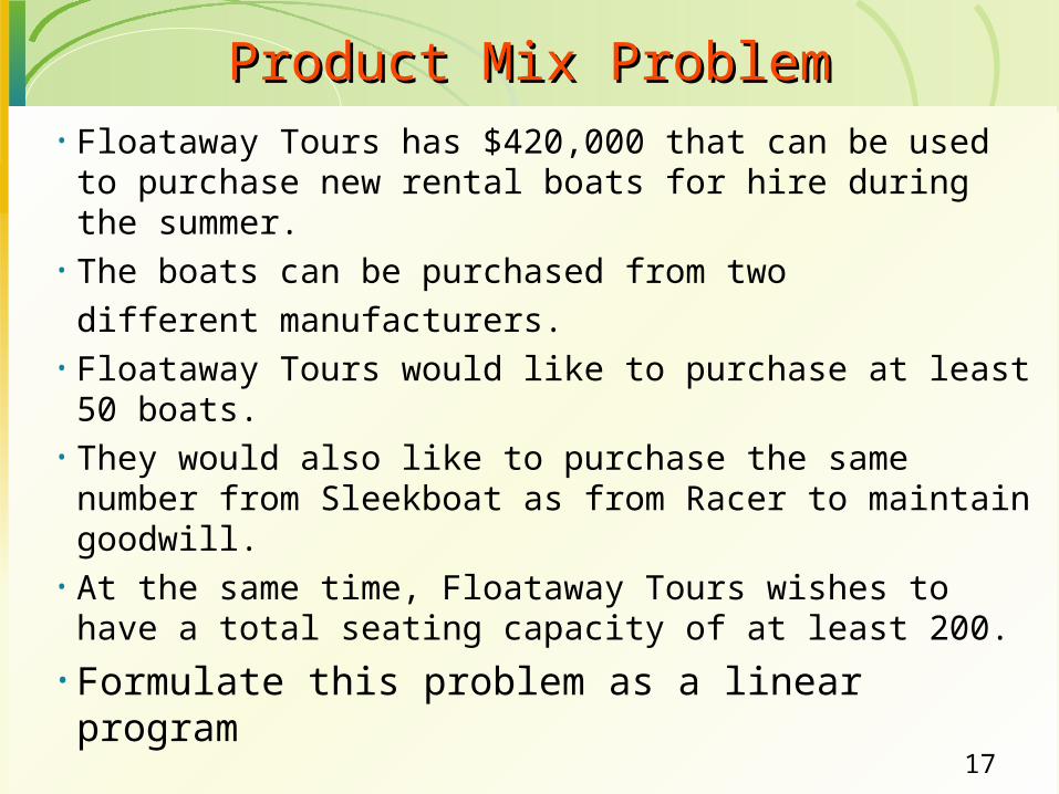
Product Mix ProblemProduct Mix Problem• Floataway Tours has $420,000 that can be used to
purchase new rental boats for hire during the summer. • The boats can be purchased from two
different manufacturers.• Floataway Tours would like to purchase at least 50 boats.• They would also like to purchase the same number from
Sleekboat as from Racer to maintain goodwill. • At the same time, Floataway Tours wishes to have a total
seating capacity of at least 200.
• Formulate this problem as a linear program
18
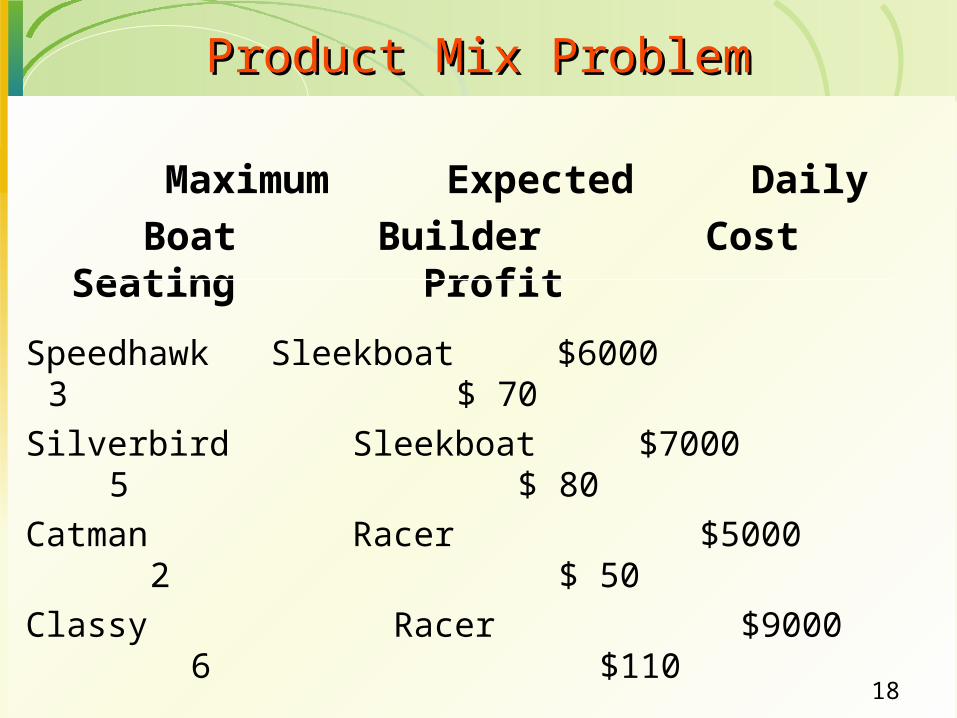
Maximum Expected Daily
Boat Builder Cost Seating Profit
Speedhawk Sleekboat $6000 3 $ 70
Silverbird Sleekboat $7000 5 $ 80
Catman Racer $5000 2 $ 50
Classy Racer $9000 6 $110
Product Mix ProblemProduct Mix Problem
19
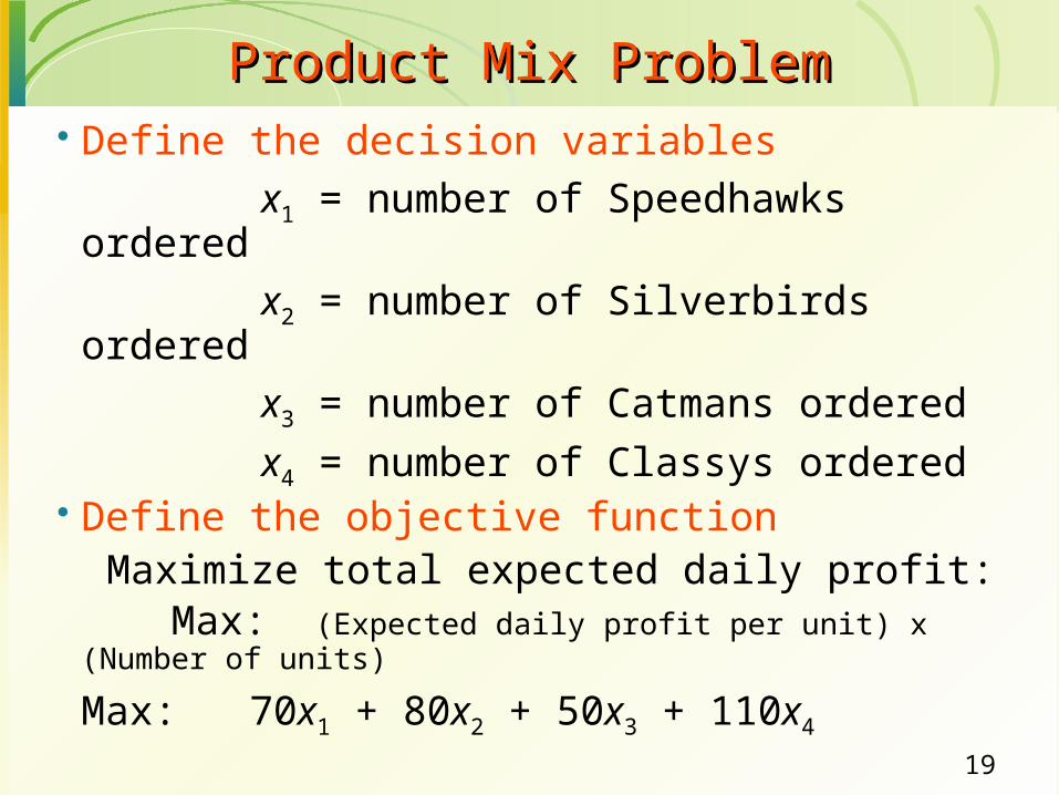
Define the decision variables
x1 = number of Speedhawks ordered
x2 = number of Silverbirds ordered
x3 = number of Catmans ordered
x4 = number of Classys ordered Define the objective function Maximize total expected daily profit: Max: (Expected daily profit per unit) x (Number of units)
Max: 70x1 + 80x2 + 50x3 + 110x4
Product Mix ProblemProduct Mix Problem

20
Define the constraints(1) Spend no more than $420,000:
6000x1 + 7000x2 + 5000x3 + 9000x4 < 420,000 (2) Purchase at least 50 boats: x1 + x2 + x3 + x4 > 50 (3) Number of boats from Sleekboat equals number
of boats from Racer: x1 + x2 = x3 + x4 or x1 + x2 - x3 - x4 = 0
(4) Capacity at least 200: 3x1 + 5x2 + 2x3 + 6x4 > 200
Nonnegativity of variables: xj > 0, for j = 1,2,3,4
Product Mix ProblemProduct Mix Problem
21
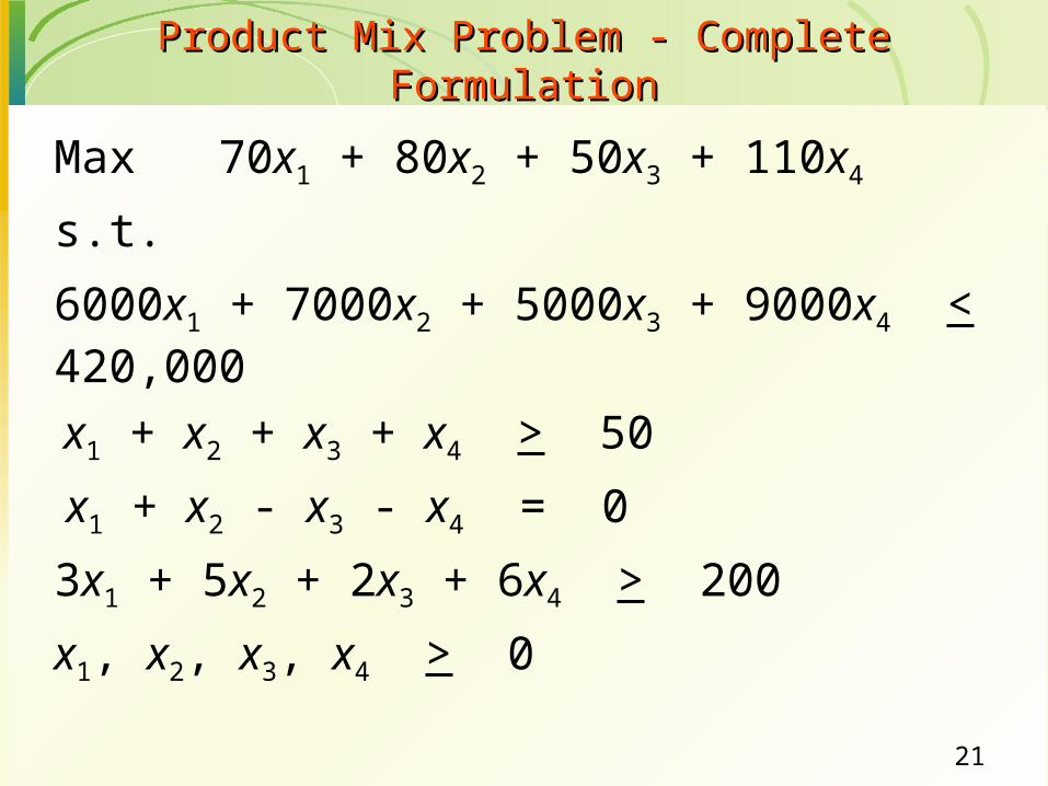
Max 70x1 + 80x2 + 50x3 + 110x4
s.t.
6000x1 + 7000x2 + 5000x3 + 9000x4 < 420,000
x1 + x2 + x3 + x4 > 50
x1 + x2 - x3 - x4 = 0
3x1 + 5x2 + 2x3 + 6x4 > 200
x1, x2, x3, x4 > 0
Product Mix Problem - Complete FormulationProduct Mix Problem - Complete Formulation
22
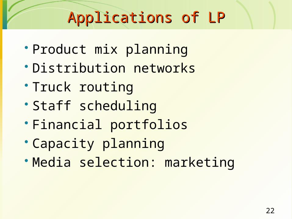
Applications of LPApplications of LP
Product mix planning Distribution networks Truck routing Staff scheduling Financial portfolios Capacity planning Media selection: marketing
23
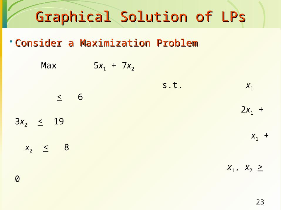
Graphical Solution of LPsGraphical Solution of LPs
Consider a Maximization ProblemConsider a Maximization Problem
Max 5x1 + 7x2
s.t. x1 < 6
2x1 + 3x2 < 19
x1 + x2 < 8
x1, x2 > 0
24 24 Slide
Slide
© 2005 Thomson/South-Western© 2005 Thomson/South-Western
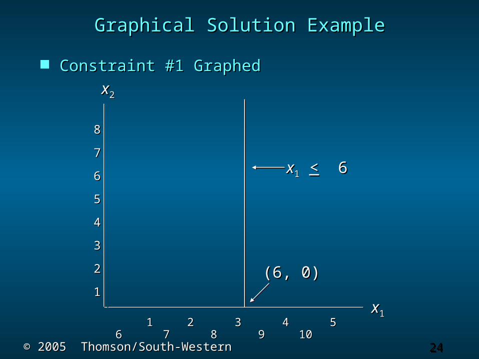
Graphical Solution ExampleGraphical Solution Example
Constraint #1 GraphedConstraint #1 Graphed
xx22
xx11
xx11 << 6 6
(6, 0)(6, 0)
88
77
66
55
44
33
22
11
1 2 3 4 5 6 7 8 9 101 2 3 4 5 6 7 8 9 10

25 25 Slide
Slide
© 2005 Thomson/South-Western© 2005 Thomson/South-Western
Graphical Solution ExampleGraphical Solution Example
Constraint #2 GraphedConstraint #2 Graphed
22xx11 + 3 + 3xx22 << 19 19
xx22
xx11
(0, 6 (0, 6 1/31/3))
(9 (9 1/21/2, 0), 0)
88
77
66
55
44
33
22
11
1 2 3 4 5 6 7 8 9 101 2 3 4 5 6 7 8 9 10
26 26 Slide
Slide
© 2005 Thomson/South-Western© 2005 Thomson/South-Western
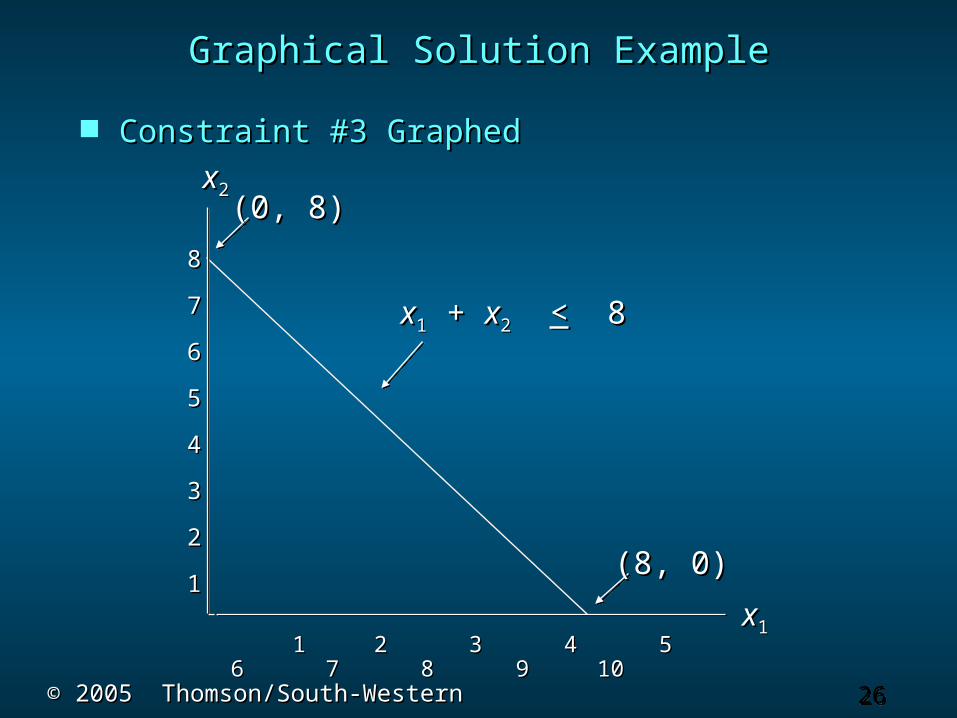
Graphical Solution ExampleGraphical Solution Example
Constraint #3 GraphedConstraint #3 Graphed
xx22
xx11
xx11 + + xx22 << 8 8
(0, 8)(0, 8)
(8, 0)(8, 0)
88
77
66
55
44
33
22
11
1 2 3 4 5 6 7 8 9 101 2 3 4 5 6 7 8 9 10
27 27 Slide
Slide
© 2005 Thomson/South-Western© 2005 Thomson/South-Western
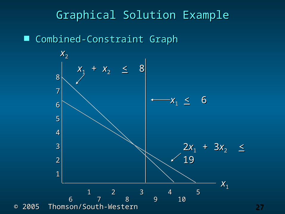
Graphical Solution ExampleGraphical Solution Example
Combined-Constraint GraphCombined-Constraint Graph
22xx11 + 3 + 3xx22 << 19 19
xx22
xx11
xx11 + + xx22 << 8 8
xx11 << 6 6
88
77
66
55
44
33
22
11
1 2 3 4 5 6 7 8 9 101 2 3 4 5 6 7 8 9 10
28 28 Slide
Slide
© 2005 Thomson/South-Western© 2005 Thomson/South-Western
88
77
66
55
44
33
22
11
1 2 3 4 5 6 7 8 9 101 2 3 4 5 6 7 8 9 10
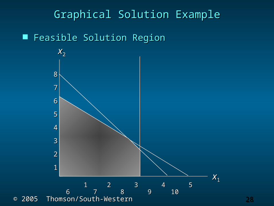
Graphical Solution ExampleGraphical Solution Example
Feasible Solution RegionFeasible Solution Region
xx11
FeasibleFeasibleRegionRegion
xx22
29 29 Slide
Slide
© 2005 Thomson/South-Western© 2005 Thomson/South-Western
88
77
66
55
44
33
22
11
1 2 3 4 5 6 7 8 9 101 2 3 4 5 6 7 8 9 10
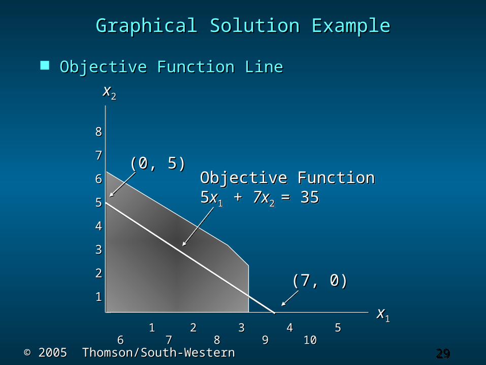
Graphical Solution ExampleGraphical Solution Example
Objective Function LineObjective Function Line
xx11
xx22
(7, 0)(7, 0)
(0, 5)(0, 5)Objective FunctionObjective Function55xx11 + + 7x7x2 2 = 35= 35Objective FunctionObjective Function55xx11 + + 7x7x2 2 = 35= 35
30 30 Slide
Slide
© 2005 Thomson/South-Western© 2005 Thomson/South-Western
88
77
66
55
44
33
22
11
1 2 3 4 5 6 7 8 9 101 2 3 4 5 6 7 8 9 10
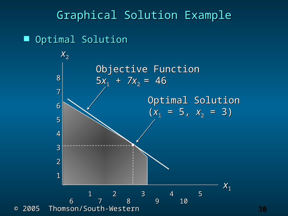
Graphical Solution ExampleGraphical Solution Example
Optimal SolutionOptimal Solution
xx11
xx22
Objective FunctionObjective Function55xx11 + + 7x7x2 2 = 46= 46Objective FunctionObjective Function55xx11 + + 7x7x2 2 = 46= 46
Optimal SolutionOptimal Solution((xx11 = 5, = 5, xx22 = 3) = 3)Optimal SolutionOptimal Solution((xx11 = 5, = 5, xx22 = 3) = 3)
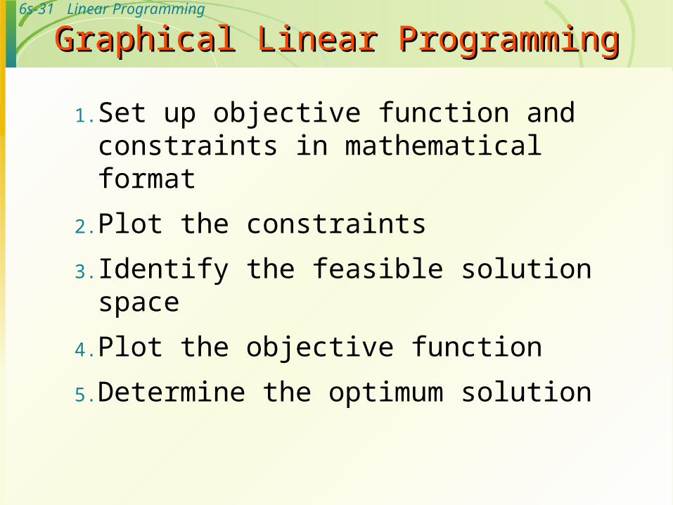
6s-31 Linear Programming
1. Set up objective function and constraints in mathematical format
2. Plot the constraints
3. Identify the feasible solution space
4. Plot the objective function
5. Determine the optimum solution
Graphical Linear ProgrammingGraphical Linear Programming
32
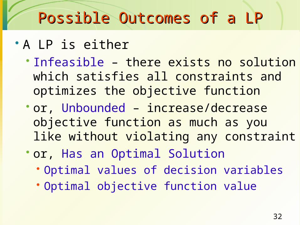
Possible Outcomes of a LPPossible Outcomes of a LP
A LP is either Infeasible – there exists no solution which satisfies
all constraints and optimizes the objective function or, Unbounded – increase/decrease objective
function as much as you like without violating any constraint
or, Has an Optimal Solution Optimal values of decision variables Optimal objective function value

33
Infeasible LP – An ExampleInfeasible LP – An Example minimize
4x11+7x12+7x13+x14+12x21+3x22+8x23+8x24+8x31+10x32+16x33+5x34
Subject to x11+x12+x13+x14=100 x21+x22+x23+x24=200 x31+x32+x33+x34=150
x11+x21+x31=80 x12+x22+x32=90 x13+x23+x33=120 x14+x24+x34=170
xij>=0, i=1,2,3; j=1,2,3,4
Total demand exceeds total supply
34
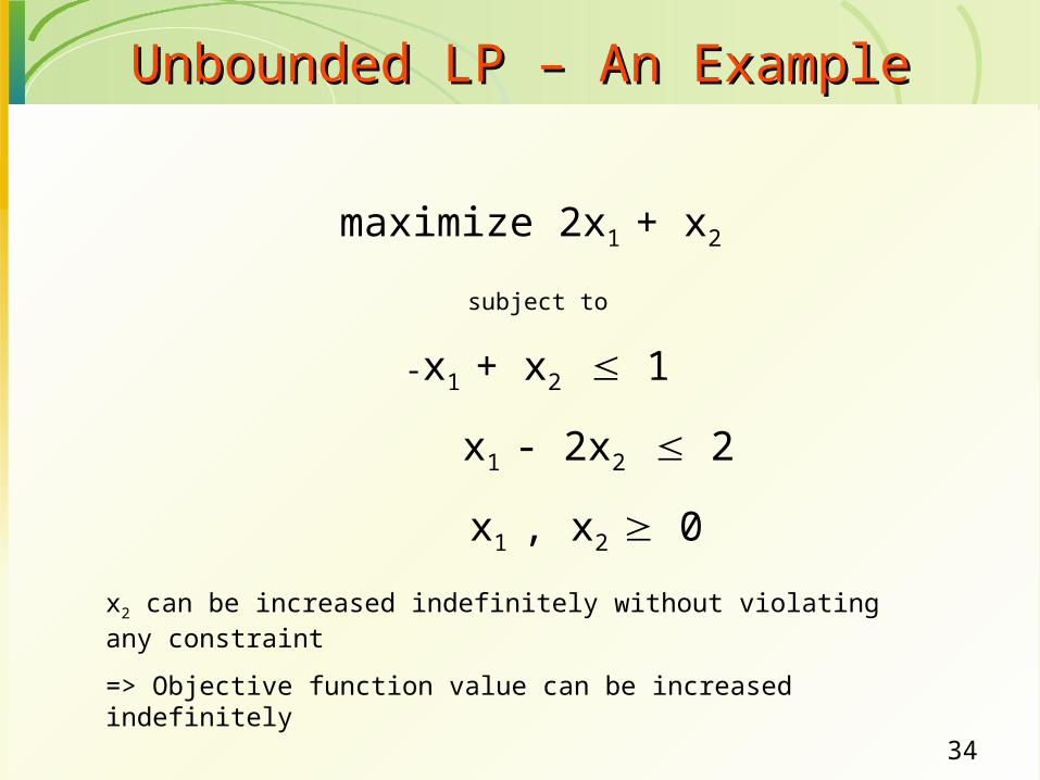
Unbounded LP – An ExampleUnbounded LP – An Example
maximize 2x1 + x2
subject to
-x1 + x2 1
x1 - 2x2 2
x1 , x2 0
x2 can be increased indefinitely without violating any constraint
=> Objective function value can be increased indefinitely
35
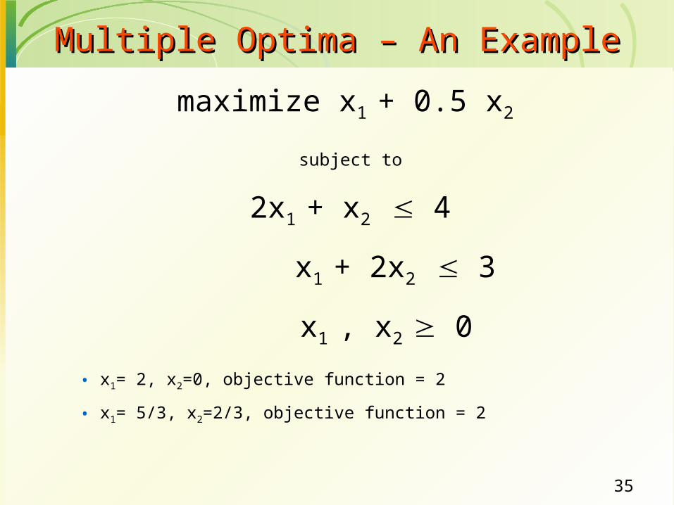
Multiple Optima – An ExampleMultiple Optima – An Example
maximize x1 + 0.5 x2
subject to
2x1 + x2 4
x1 + 2x2 3
x1 , x2 0
• x1= 2, x2=0, objective function = 2
• x1= 5/3, x2=2/3, objective function = 2
36
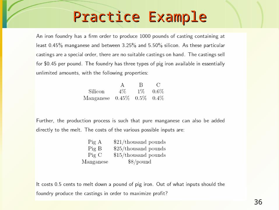
Practice ExamplePractice Example