1

Javier AparicioDivisión de Estudios Políticos, CIDE

javier.aparicio@cide.edu

Otoño 2008

http://www.cide.edu/investigadores/aparicio/metodos.html

Regresión Lineal Múltiple

yi = 0 + 1x1i + 2x2i + . . . kxki + ui

B. Inferencia

2

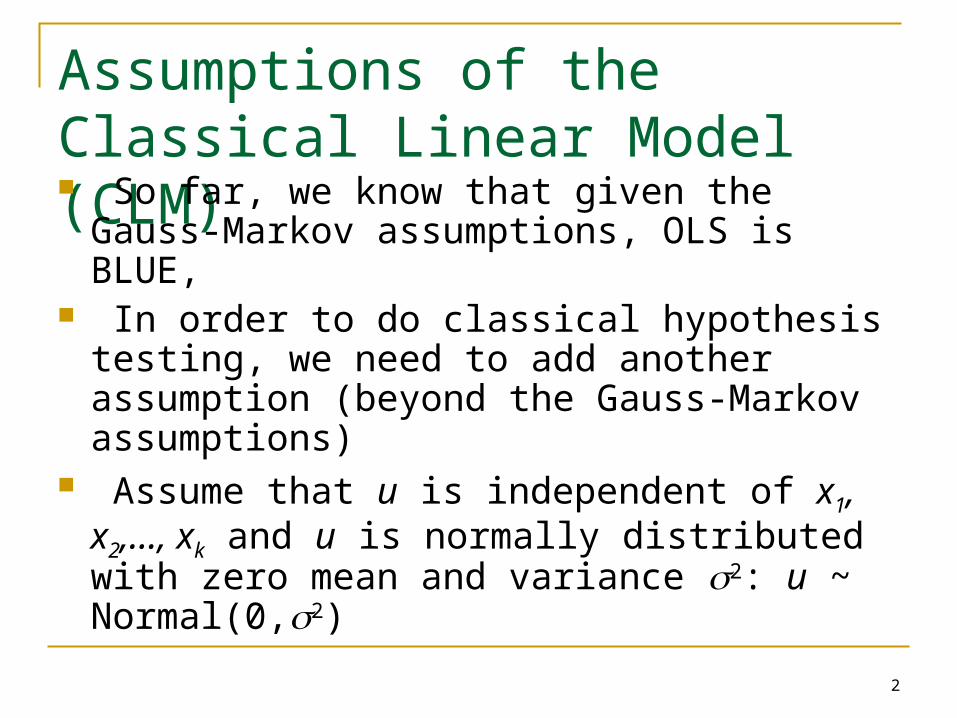
Assumptions of the Classical Linear Model (CLM) So far, we know that given the Gauss-

Markov assumptions, OLS is BLUE, In order to do classical hypothesis testing,

we need to add another assumption (beyond the Gauss-Markov assumptions)

Assume that u is independent of x1, x2,…, xk and u is normally distributed with zero mean and variance 2: u ~ Normal(0,2)

3

CLM Assumptions (cont)

Under CLM, OLS is not only BLUE, but is the minimum variance unbiased estimator

We can summarize the population assumptions of CLM as follows

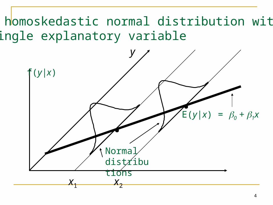
y|x ~ Normal(0 + 1x1 +…+ kxk, 2) While for now we just assume normality,

clear that sometimes not the case Large samples will let us drop normality

4

..

x1 x2

The homoskedastic normal distribution with a single explanatory variable

E(y|x) = 0 + 1x

y

f(y|x)

Normaldistributions

5

Normal Sampling Distributions

errors theofn combinatiolinear a is

it becausenormally ddistribute is ˆ

0,1Normal ~ ˆˆ

thatso ,ˆ,Normal ~ˆ

st variableindependen theof valuessample the

on lconditiona s,assumption CLM Under the

j

j

jj

jjj

sd

Var

6

The t Test

1:freedom of degrees theNote

ˆby estimate tohave webecause

normal) (vson distributi a is thisNote

~ ˆˆ

sassumption CLM Under the

22

1j

kn

t

tse kn

j

j

7

The t Test (cont)

Knowing the sampling distribution for the standardized estimator allows us to carry out hypothesis tests

Start with a null hypothesis For example, H0: j=0

If accept null, then accept that xj has no effect on y, controlling for other x’s

8

The t Test (cont)

0

ˆj

H ,hypothesis null accept the

o whether tdetermine torulerejection a

withalong statistic our use then willWe

ˆˆ

: ˆfor statistic the""

form toneedfirst eour test w perform To

t

sett

j

j

j

9

t Test: One-Sided Alternatives Besides our null, H0, we need an alternative

hypothesis, H1, and a significance level H1 may be one-sided, or two-sided H1: j > 0 and H1: j < 0 are one-sided H1: j 0 is a two-sided alternative If we want to have only a 5% probability of

rejecting H0 if it is really true, then we say our significance level is 5%

10

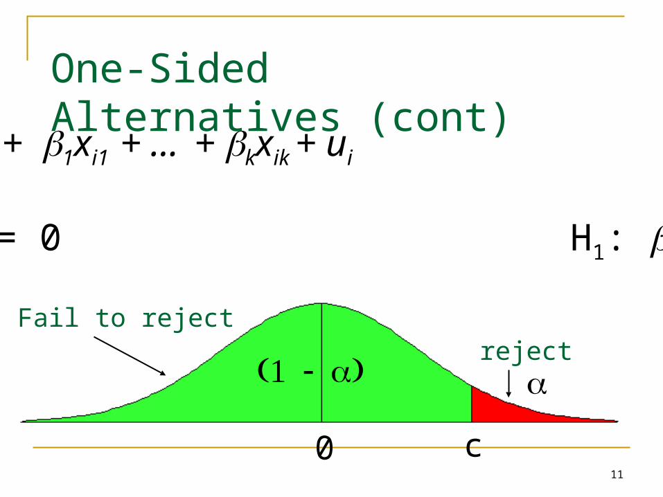
One-Sided Alternatives (cont)

Having picked a significance level, , we look up the (1 – )th percentile in a t distribution with n – k – 1 df and call this c, the critical value

We can reject the null hypothesis if the t statistic is greater than the critical value

If the t statistic is less than the critical value then we fail to reject the null

11

yi = 0 + 1xi1 + … + kxik + ui

H0: j = 0 H1: j > 0

c0

One-Sided Alternatives (cont)

Fail to rejectreject

12

One-sided vs Two-sided

Because the t distribution is symmetric, testing H1: j < 0 is straightforward. The critical value is just the negative of before

We can reject the null if the t statistic < –c, and if the t statistic > than –c then we fail to reject the null

For a two-sided test, we set the critical value based on /2 and reject H1: j 0 if the absolute value of the t statistic > c

13

yi = 0 + 1Xi1 + … + kXik + ui

H0: j = 0 H1: j > 0

c0

-c

Two-Sided Alternatives

reject reject

fail to reject

14

Summary for H0: j = 0

Unless otherwise stated, the alternative is assumed to be two-sided

If we reject the null, we typically say “xj is statistically significant at the % level”

If we fail to reject the null, we typically say “xj is statistically insignificant at the % level”

15

Testing other hypotheses

A more general form of the t statistic recognizes that we may want to test something like H0: j = aj

In this case, the appropriate t statistic is

teststandard for the 0

where,ˆˆ

j

j

jj

a

sea

t

16

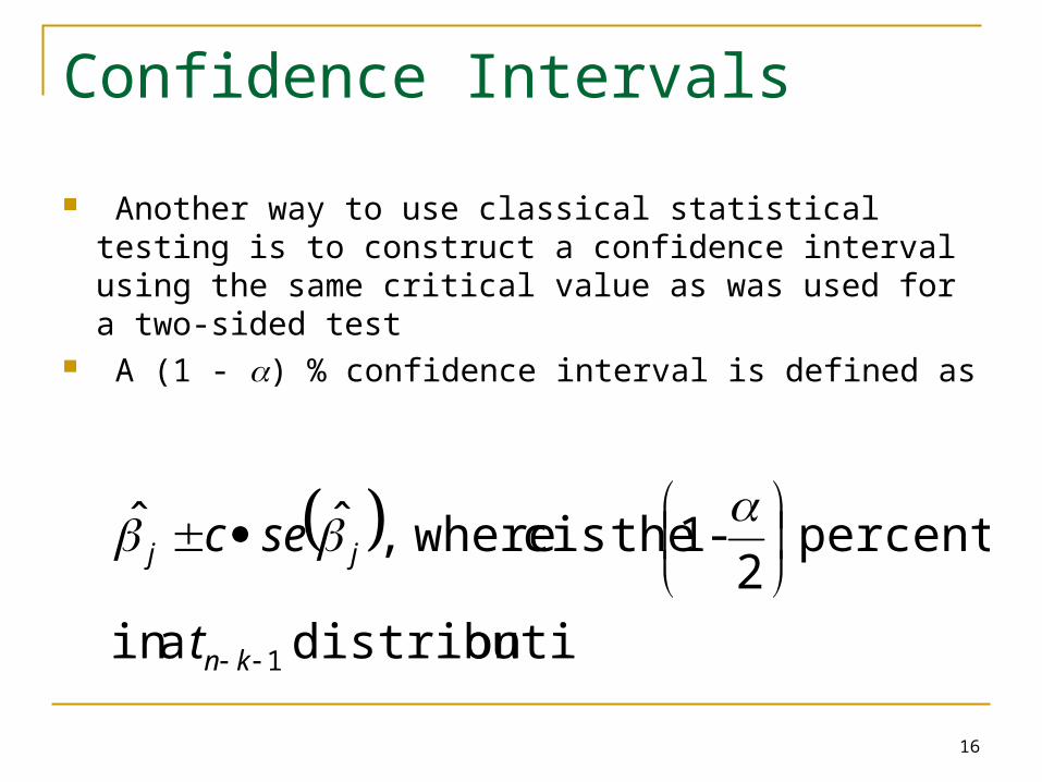
Confidence Intervals

Another way to use classical statistical testing is to construct a confidence interval using the same critical value as was used for a two-sided test

A (1 - ) % confidence interval is defined as

ondistributi ain

percentile 2

-1 theis c where,ˆˆ

1

kn

jj

t

sec

17

Computing p-values for t tests An alternative to the classical approach is to

ask, “what is the smallest significance level at which the null would be rejected?”

So, compute the t statistic, and then look up what percentile it is in the appropriate t distribution – this is the p-value

p-value is the probability we would observe the t statistic we did, if the null were true

18

Stata and p-values, t tests, etc. Most computer packages will compute the p-

value for you, assuming a two-sided test If you really want a one-sided alternative,

just divide the two-sided p-value by 2 Stata provides the t statistic, p-value, and

95% confidence interval for H0: j = 0 for you, in columns labeled “t”, “P > |t|” and “[95% Conf. Interval]”, respectively

19

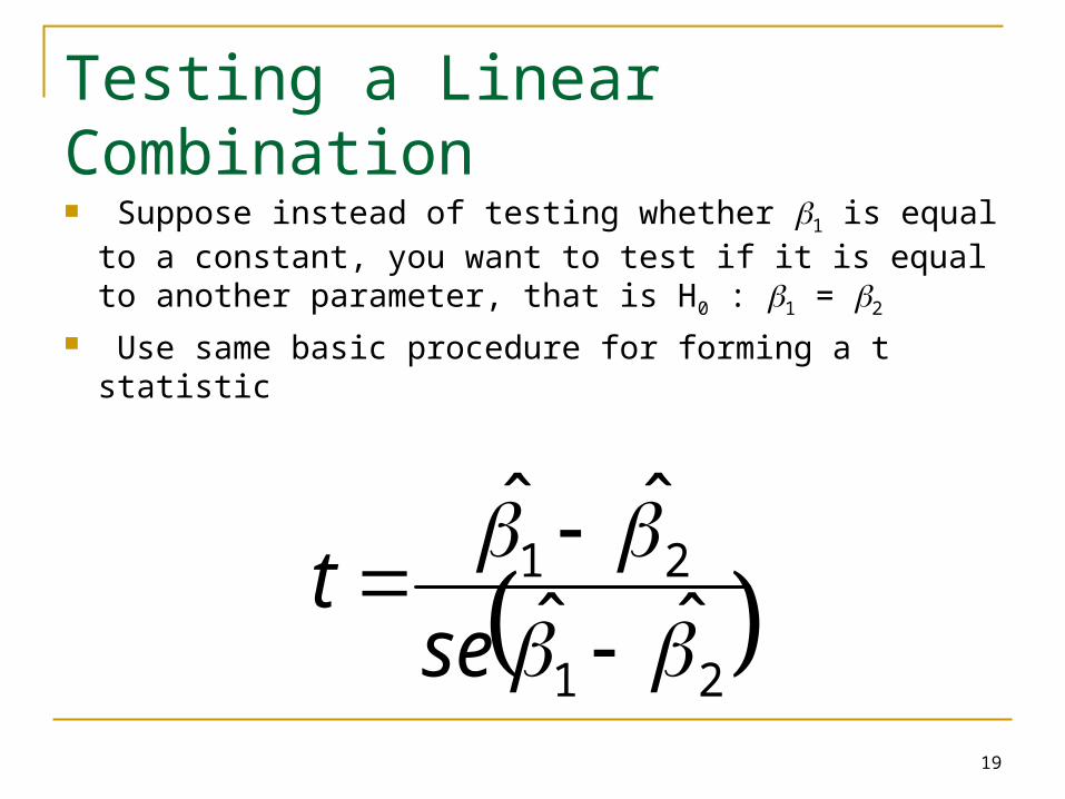
Testing a Linear Combination Suppose instead of testing whether 1 is equal to a

constant, you want to test if it is equal to another parameter, that is H0 : 1 = 2

Use same basic procedure for forming a t statistic

21

21

ˆˆ

ˆˆ

se

t

20

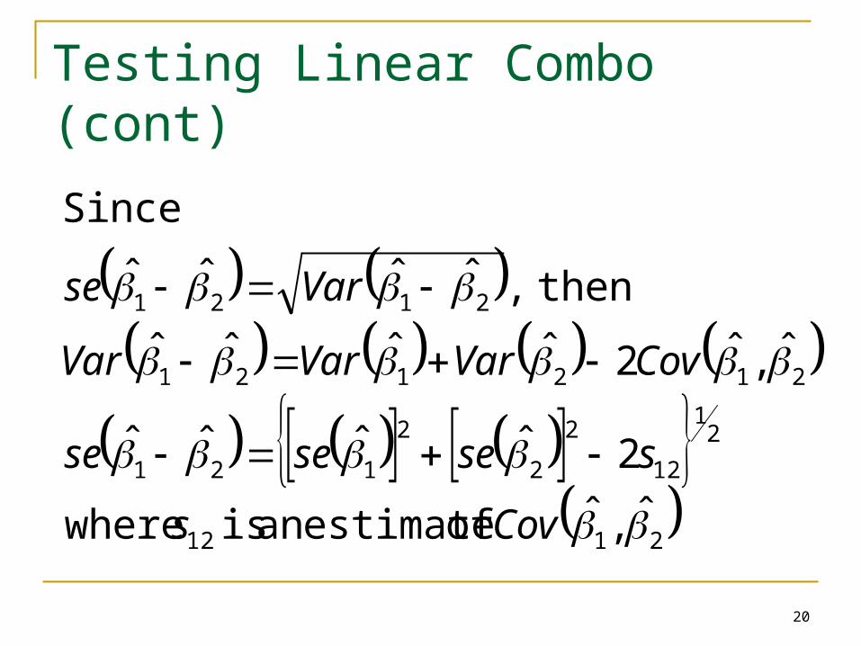
Testing Linear Combo (cont)

2112

21

12

2

2

2

121

212121

2121

ˆ,ˆ of estimatean is where

2ˆˆˆˆ

ˆ,ˆ2ˆˆˆˆ

then,ˆˆˆˆ

Since

Covs

ssesese

CovVarVarVar

Varse

21

Testing a Linear Combo (cont) So, to use formula, need s12, which standard

output does not have Many packages will have an option to get it,

or will just perform the test for you In Stata, after reg y x1 x2 … xk you would

type test x1 = x2 to get a p-value for the test More generally, you can always restate the

problem to get the test you want

22

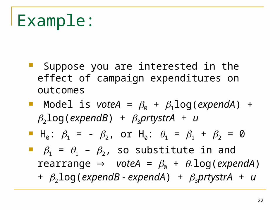
Example:

Suppose you are interested in the effect of campaign expenditures on outcomes

Model is voteA = 0 + 1log(expendA) + 2log(expendB) + 3prtystrA + u

H0: 1 = - 2, or H0: 1 = 1 + 2 = 0

1 = 1 – 2, so substitute in and rearrange voteA = 0 + 1log(expendA) + 2log(expendB - expendA) + 3prtystrA + u

23

Example (cont):

This is the same model as originally, but now you get a standard error for 1 – 2 = 1 directly from the basic regression

Any linear combination of parameters could be tested in a similar manner

Other examples of hypotheses about a single linear combination of parameters: 1 = 1 + 2 ; 1 = 52 ; 1 = -1/22 ; etc

24

Multiple Linear Restrictions

Everything we’ve done so far has involved testing a single linear restriction, (e.g. 1 = or 1 = 2 )

However, we may want to jointly test multiple hypotheses about our parameters

A typical example is testing “exclusion restrictions” – we want to know if a group of parameters are all equal to zero

25

Testing Exclusion Restrictions Now the null hypothesis might be something

like H0: k-q+1 = 0, , k = 0 The alternative is just H1: H0 is not true Can’t just check each t statistic separately,

because we want to know if the q parameters are jointly significant at a given level – it is possible for none to be individually significant at that level

26

Exclusion Restrictions (cont)

To do the test we need to estimate the “restricted model” without xk-q+1,, …, xk included, as well as the “unrestricted model” with all x’s included

Intuitively, we want to know if the change in SSR is big enough to warrant inclusion of xk-q+1,, …, xk

edunrestrict isur and restricted isr

where,1

knSSR

qSSRSSRF

ur

urr

27

The F statistic

The F statistic is always positive, since the SSR from the restricted model can’t be less than the SSR from the unrestricted

Essentially the F statistic is measuring the relative increase in SSR when moving from the unrestricted to restricted model

q = number of restrictions, or dfr – dfur

n – k – 1 = dfur

28

The F statistic (cont)

To decide if the increase in SSR when we move to a restricted model is “big enough” to reject the exclusions, we need to know about the sampling distribution of our F stat

Not surprisingly, F ~ Fq,n-k-1, where q is referred to as the numerator degrees of freedom and n – k – 1 as the denominator degrees of freedom

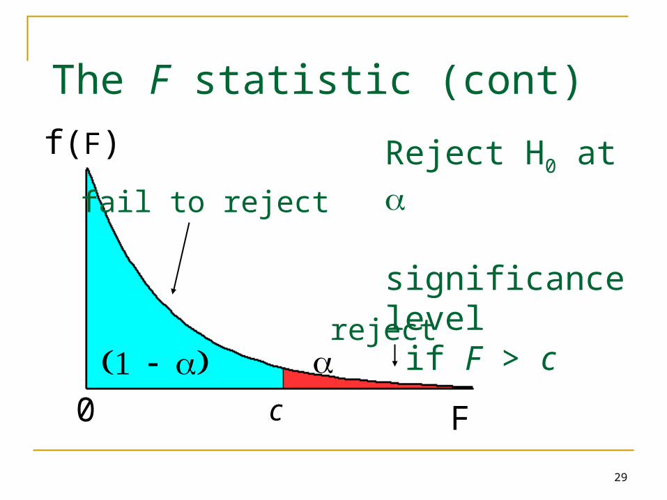
29

0 c

f(F)

F

The F statistic (cont)

reject

fail to reject

Reject H0 at significance level if F > c

30

The R2 form of the F statistic

Because the SSR’s may be large and unwieldy, an alternative form of the formula is useful

We use the fact that SSR = SST(1 – R2) for any regression, so can substitute in for SSRu and SSRur

edunrestrict isur and restricted isr

again where,11 2

22

knR

qRRF

ur

rur

31

Overall Significance

A special case of exclusion restrictions is to test H0: 1 = 2 =…= k = 0

Since the R2 from a model with only an intercept will be zero, the F statistic is simply

11 2

2

knR

kRF

32

General Linear Restrictions

The basic form of the F statistic will work for any set of linear restrictions

First estimate the unrestricted model and then estimate the restricted model

In each case, make note of the SSR Imposing the restrictions can be tricky – will

likely have to redefine variables again

33

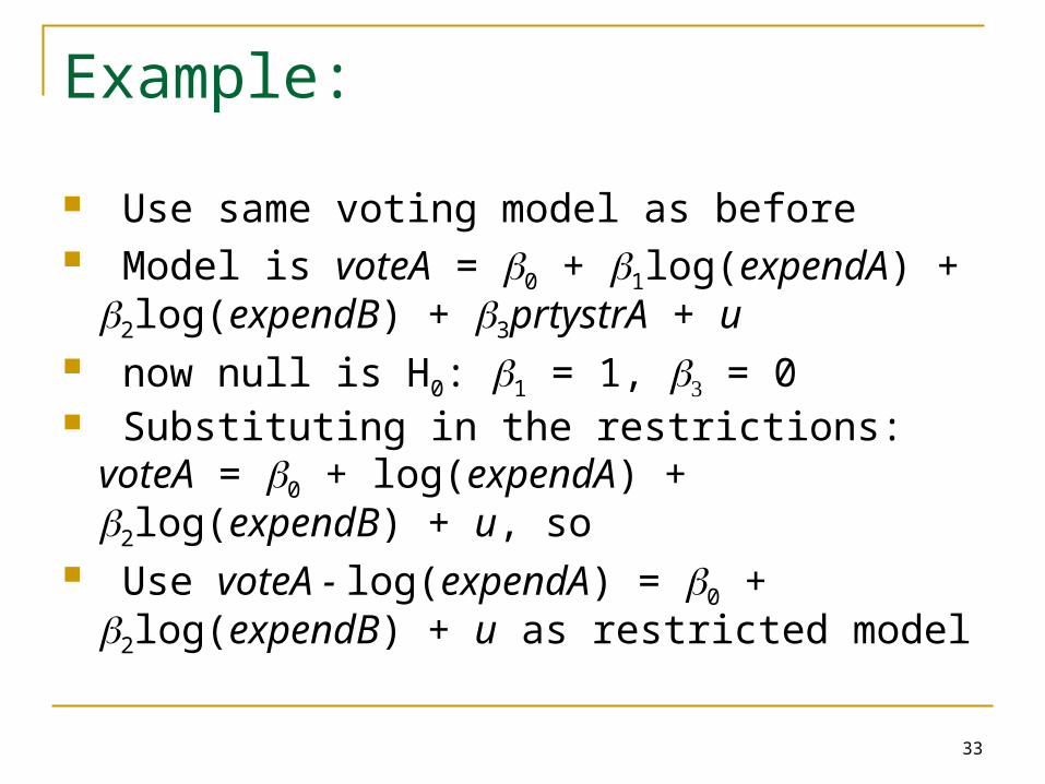
Example:

Use same voting model as before Model is voteA = 0 + 1log(expendA) +

2log(expendB) + 3prtystrA + u now null is H0: 1 = 1, = 0 Substituting in the restrictions: voteA = 0 +

log(expendA) + 2log(expendB) + u, so Use voteA - log(expendA) = 0 +

2log(expendB) + u as restricted model

34

F Statistic Summary

Just as with t statistics, p-values can be calculated by looking up the percentile in the appropriate F distribution

Stata will do this by entering: display fprob(q, n – k – 1, F), where the appropriate values of F, q,and n – k – 1 are used

If only one exclusion is being tested, then F = t2, and the p-values will be the same