1 J. Stat .Mec h.for this simple system was shown to be remarkably com plex, with three distinct...

J.Stat.M

ech.(2005)

P12003

ournal of Statistical Mechanics:An IOP and SISSA journalJ Theory and Experiment

Simulation results for an interactingpair of resistively shunted Josephsonjunctions

Philipp Werner1, Gil Refael2,3 and Matthias Troyer1

1 Institut fur Theoretische Physik, ETH Honggerberg, CH-8093 Zurich,Switzerland2 Kavli Institute of Theoretical Physics, University of California,Santa Barbara, CA 93106, USA3 Department of Physics, California Institute of Technology, Pasadena,CA 91125, USAE-mail: [email protected], [email protected] [email protected]

Received 11 August 2005Accepted 2 November 2005Published 5 December 2005

Online at stacks.iop.org/JSTAT/2005/P12003doi:10.1088/1742-5468/2005/12/P12003

Abstract. Using a new cluster Monte Carlo algorithm, we study the phasediagram and critical properties of an interacting pair of resistively shuntedJosephson junctions. This system models tunnelling between two electrodesthrough a small superconducting grain, and is described by a double sine-Gordonmodel. In accordance with theoretical predictions, we observe three differentphases and crossover effects arising from an intermediate coupling fixed point.On the superconductor-to-metal phase boundary, the observed critical behaviouris within error-bars the same as in a single junction, with identical values of thecritical resistance and a correlation function exponent which depends only on thestrength of the Josephson coupling. We explain these critical properties on thebasis of a renormalization group (RG) calculation. In addition, we propose analternative new mean-field theory for this transition, which correctly predicts thelocation of the phase boundary at intermediate Josephson coupling strength.

Keywords: dissipative systems (theory), quantum Monte Carlo simulations,quantum phase transitions (theory)

ArXiv ePrint: cond-mat/0508163

c©2005 IOP Publishing Ltd 1742-5468/05/P12003+42$30.00

mailto:[email protected]



http://stacks.iop.org/JSTAT/2005/P12003

http://dx.doi.org/10.1088/1742-5468/2005/12/P12003

http://arxiv.org/abs/cond-mat/0508163

J.Stat.M

ech.(2005)

P12003

Simulation results for an interacting pair of resistively shunted Josephson junctions

Contents

1. Introduction 2

2. Theory for the symmetric two-junction system 52.1. Effective action . . . . . . . . . . . . . . . . . . . . . . . . . . . . . . . . . 62.2. Weak coupling limit . . . . . . . . . . . . . . . . . . . . . . . . . . . . . . . 62.3. Strong coupling limit . . . . . . . . . . . . . . . . . . . . . . . . . . . . . . 82.4. Intermediate coupling fixed point (ICFP) region . . . . . . . . . . . . . . . 11

3. Monte Carlo method 13

4. Phase diagram 154.1. Simulation results . . . . . . . . . . . . . . . . . . . . . . . . . . . . . . . . 154.2. Crossover effects in the Monte Carlo results . . . . . . . . . . . . . . . . . 20

5. The critical two-junction system in the ICFP region—comparison with a singleJosephson junction 235.1. Numerical results and resemblance to the single junction . . . . . . . . . . 235.2. RG analysis of the critical effective resistance in the two-junction system . 27

6. The ICFP as a self-consistent fixed point 29

7. Correlation function in the NOR phase 33

8. Conclusions 36

Acknowledgments 37

Appendix A: Critical exponents of the ICFP 38A.1 Weak coupling . . . . . . . . . . . . . . . . . . . . . . . . . . . . . . . 38A.2 Strong coupling regime . . . . . . . . . . . . . . . . . . . . . . . . . . 39

Appendix B: Approximate calculation of the NOR–FSC phase boundary 40

Appendix C: Solution of the circuit in figure 21 41

References 41

1. Introduction

The effects of dissipation and decoherence are ubiquitous in quantum systems andinfluence the properties of materials and nanoscale devices in a profound way. Already thesimplest model system, an Ising spin in a transverse field which is coupled to an ohmic heatbath, displays interesting behaviour such as a dynamical phase transition to a localizedstate at a critical value of the dissipation strength [2]. Another prominent example isthe resistively shunted Josephson junction, which undergoes a superconductor-to-metaltransition at a critical value of the shunt resistance [3]–[6], which equals the quantum ofresistance RQ = h/4e2 = 6.5 kΩ. Arrays of Josephson junctions with dissipation havebeen studied both as a model for granular superconducting films or nanowires [7]–[9],

doi:10.1088/1742-5468/2005/12/P12003 2

http://dx.doi.org/10.1088/1742-5468/2005/12/P12003

J.Stat.M

ech.(2005)

P12003


C

RR

EJr

E

EJ

EC

Rjunction RjunctionRlead

Figure 1. Upper figure: two-junction model considered in [1] with identicalshunt resistors R for the left and right junction. The dotted box representsthe central grain which incorporates a phenomenological charge relaxationmechanism described by the resistance r. Lower figure: equivalent modelwith modified shunt resistors Rjunction = R + 2r and an additional resistorRlead = (R/r)(R + 2r) connecting the leads.

and in their own right [10, 11]. The behaviour of these systems, and in particular theirsuperconductor-to-metal phase transition, is far from being completely understood.

Recently, Refael et al have studied a model of a mesoscopic superconducting grainconnected to two leads via Josephson tunnelling and shunt resistors [1]. The phase diagramfor this simple system was shown to be remarkably complex, with three distinct phases.In addition, contrary to the case of a single resistively shunted Josephson junction, one ofthe phase boundaries is controlled in part by an intermediate coupling fixed point, and thesuperconductor-to-normal transition across this boundary can be tuned by the Josephsonenergy itself. The above effects indicate that although the system discussed in [1] is zerodimensional, it nearly has the full complexity of a one-dimensional array of Josephsonjunctions. Much of the recent results on Josephson junction chains in [12] draw directlyfrom the two-junction system. The renormalization group (RG) flow equations of thetwo-junction system are also nearly identical to those of the two-dimensional triangularlattice presented in [13]. In this closely related work on Josephson junction arrays, thelocal nature of the phase transition, as well as floating phases, have been discussed.

The development of a powerful new cluster Monte Carlo algorithm [14] has allowedus to test and verify several analytical predictions for the single junction and to observecontinuously varying correlation exponents along the phase boundary. In this paper wewill use adapted versions of these cluster moves to simulate the two-junction model of [1],which is the simplest extension of the single-junction case which exhibits interesting newphysics. The model (with identical shunt resistors) is shown in the upper part of figure 1. Itconsists of two Josephson junctions with coupling energy EJ, each shunted with an ohmic

doi:10.1088/1742-5468/2005/12/P12003 3

http://dx.doi.org/10.1088/1742-5468/2005/12/P12003

J.Stat.M

ech.(2005)

P12003


*

Q

R =r+RQ

1

u=0

NOR

ICFP

w=0

u=0

FSC

2

1/2 1

w=

0 R =(2rR+R )/(R+r)Q

R/RQ

r/RQ

SC

R =r+R/2

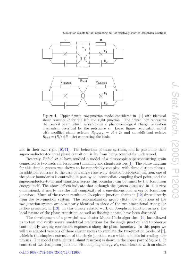
Figure 2. Phase diagram in the limits EJ/EC 1 (solid lines) and EJ/EC 1(solid and dashed lines). Besides the superconducting (FSC) and metallic (NOR)phase, the two-junction system can be in a state which is superconductingfrom lead to lead, although the individual junctions are insulating (SC∗). Theparameters u, w and u, w are defined in equations (22) and (26). The valuesu = 0 and w = 0 define the FSC–NOR boundary in the weak coupling limit, andu = 0 and w = 0 in the strong coupling limit.

resistor R. On the central grain, the model incorporates a ‘charge relaxation mechanism’(supposed to represent the break-up of Cooper pairs into electrons) which is described byan additional resistor r.

Dissipation produced by electrons flowing through the resistors reduces phasefluctuations between the superconducting islands which they connect. This can be seenfrom the dissipative action term in equation (4), and it explains how strong dissipationleads to superconducting phase coherence. Depending on the values of R and r, threedifferent phases occur.

• The individual junctions are insulating and there is no supercurrent from lead to lead:normal phase (NOR).

• The junctions are superconducting and thus also the whole device from lead to lead:fully superconducting phase (FSC).

• The individual junctions are insulating but there is superconducting phase coherencefrom lead to lead: SC∗ phase.

The phase diagram for the limiting cases EJ EC and EJ EC has been computedin [1] using an RG approach and is shown in figure 2 as a function of the resistances R andr. The boundary between the NOR- and FSC-phase in the region marked ICFP dependson the value of EJ/EC as well as the values of the resistors r and R. The behaviour of thesystem in this region is controlled by an intermediate coupling fixed point (ICFP), whichwill be discussed in section 2.4.

In the remains of this paper we present the results of a thorough Monte Carlo (MC)investigation of the two-junction system. Each result is compared with predictions orexplanations based on the RG flow equations presented in section 2. After discussing

doi:10.1088/1742-5468/2005/12/P12003 4

http://dx.doi.org/10.1088/1742-5468/2005/12/P12003

J.Stat.M

ech.(2005)

P12003


the various phases of the two-junction system, we explain in section 3 the Monte Carlomethod which was used to investigate the model numerically. In particular, we discussseveral types of efficient cluster updates, which are adaptations of the recently developedrejection-free cluster algorithm for single resistively shunted junctions [14].

In section 4 we identify the three phases NOR, FSC and SC∗ by computing thetemperature dependence of the lead-to-lead and lead-to-grain resistance. The numericallyobtained phase diagram at intermediate Josephson coupling is compared to the theoreticalpredictions for weak and strong Josephson coupling. There is a good agreement betweentheory and simulation results, except in the region where the three phases meet. Weexplain these small deviations of the measured phase boundaries from the predicted onesin terms of slow crossovers in the RG flow, which prevent the MC simulation from exploringthe zero-temperature behaviour.

In section 5 we concentrate on the critical FSC–NOR line in the ICFP region.In particular, we compare the critical properties of the two-junction system to thoseof a single junction with the same Josephson coupling EJ/EC, and a shunt resistanceRs = RQ. The two systems exhibit (within error-bars) identical behaviour in theircorrelation functions, fluctuations and the effective resistance of the critical junctions.These critical properties depend on the value of EJ/EC but not on the value of theresistors r and R. In section 5.2, we try to explain this rather surprising observation interms of the effective junction resistances of the two-junction system, calculated from theRG flow of section 2. We show that the predicted critical resistance exhibits only a weakdependence on the (shunt) resistors and agrees quite well with the measured value.

In section 6, however, we pursue a different path to explain the remarkableresemblance between the single resistively shunted junction and the two-junction system.We show that the data can be well explained by a ‘mean-field’ theory, which treats oneof the two junctions as an effective resistor. This is a new way of approaching the doublesine–Gordon model action (equation (1) below). The assumption is that, on the FSC–NOR phase boundary, each junction sees an environment which imitates a shunt resistorRs = RQ and that it may be replaced by a resistor whose value can be found from thecritical resistance of the single resistively shunted junction (with the same Josephsoncoupling). On the basis of these assumptions it is possible to derive an expression for theposition of the FSC–NOR phase boundary, which fits the MC data and the RG-basedpredictions quite well.

In section 6 we consider the phase–phase correlation functions in the NOR phasewithin the ICFP region. For fixed resistors, we measure a strong dependence of thecorrelation exponents on the Josephson coupling strength, which is in contrast to thesingle-junction model, where these exponents depend only on the value of the shuntresistor. This behaviour is explained as a consequence of the flow in the additionalJosephson coupling J+ between the leads, which is generated under the RG and notpresent in the single-junction model.

2. Theory for the symmetric two-junction system

In this section we will present the effective action for the symmetric two-junction system,and then briefly discuss its RG flow equations and the various phases. This discussionwill prove to be especially useful when interpreting the Monte Carlo results.

doi:10.1088/1742-5468/2005/12/P12003 5

http://dx.doi.org/10.1088/1742-5468/2005/12/P12003

J.Stat.M

ech.(2005)

P12003


We will first describe the NOR–SC∗ and SC∗–FSC transitions in the weak and strongcoupling limits. It is important to note that the SC∗ phase appears due to interactionsbetween the two junctions, and can not be understood in terms of the physics of a singlejunction. Finally, we will discuss the important intermediate coupling fixed point whichcontrols the direct NOR–FSC transition.

2.1. Effective action

The imaginary-time effective action of the symmetric two-junction system can be writtenas a functional of the phase differences φ1 and φ2 across the first and second junction,

Seff [φ1, φ2] = SC[φ1, φ2] + SJ[φ1, φ2] + SD[φ1, φ2], (1)

where the charging term SC, the Josephson coupling term SJ and the dissipation term SD

read

SC[φ1, φ2] =1

16EC

∫ β

0

dτ

[(dφ1

dτ

)2

+

(dφ2

dτ

)2], (2)

SJ[φ1, φ2] = −EJ

∫ β

0

dτ [cos(φ1) + cos(φ2)], (3)

SD[φ1, φ2] =RQ

R(R + 2r)

∫ β

0

dτ dτ ′ (π/β)2

sin2((π/β)(τ − τ ′))

× [R(φ1(τ) − φ1(τ′))2 + R(φ2(τ) − φ2(τ

′))2

+ r((φ1(τ) + φ2(τ)) − (φ1(τ′) + φ2(τ

′)))2]. (4)

EC = e2/2C is the (single-electron) charging energy of each junction and sets the overallenergy scale. EJ denotes the coupling strengths of the junctions. Ohmic dissipation inthe resistors is introduced using the model of Caldeira and Leggett [15, 16].

The system discussed in [1] is equivalent to the one illustrated in the lower part offigure 1, where each junction is shunted by a resistor

Rjunction = R + 2r (5)

and the leads are connected by an additional resistor

Rlead = (R/r)(R + 2r). (6)

This is a consequence of the ‘Y –∆’ transformation of resistor networks [1]. For simplicity,we consider a capacitive coupling between the leads and central grain only and noJosephson coupling between the leads. Such a coupling will be generated by the RGflow.

2.2. Weak coupling limit

When the Josephson coupling energy EJ is small, it can be used as a small parameterfor a perturbative RG analysis. As explained in [1], in addition to the bare Josephsonenergy of the two junctions, the RG flow produces yet another Josephson coupling—theco-tunnelling J+. In the same sense that EJ is the amplitude for a pair-hopping betweenthe leads and the grain, J+ is the amplitude for a Cooper pair to tunnel between the two

doi:10.1088/1742-5468/2005/12/P12003 6

http://dx.doi.org/10.1088/1742-5468/2005/12/P12003

J.Stat.M

ech.(2005)

P12003


J+

A B C

J J2e 2e

2e

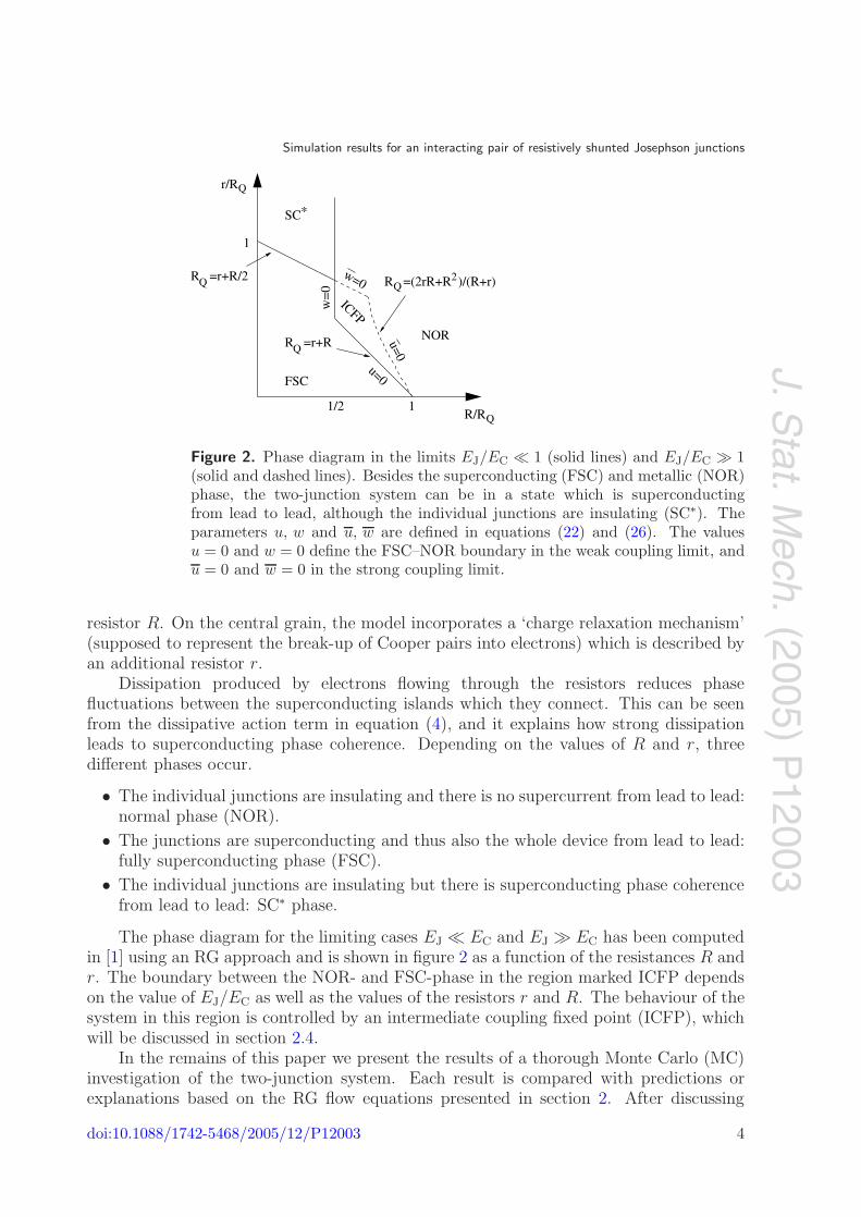
Figure 3. In the weak coupling limit, we consider the RG flow of the Josephsoncouplings J (with J0 = EJ) and J+. J is the amplitude for Cooper-pair hoppingbetween either of the leads and the grain. J+ is the amplitude for Cooper-pairtunnelling from lead to lead. This process is generated in the second order of theRG flow.

leads, skipping over the grain (see figure 3). To be more specific, the Cooper-pair hoppingconductivities are

GAB = GBC ∼ E2J , GAC ∼ J2

+. (7)

Let us quote here the RG equations for the Josephson strengths in the symmetriccase [1]. To distinguish between the bare Josephson energy EJ and the renormalized one,we use J to denote the flow of EJ. For the Josephson strengths J of the junction and J+

between the leads we getdJ

dl= J

(1 − R + r

RQ

)+

R

RQJJ+, (8)

dJ+

dl= J+

(1 − 2R

RQ

)+

r

RQJ2. (9)

The Josephson coupling J+ between the leads is originally zero, but will be generatedunder the flow in the second order in J . From these RG equations we can infer the scalingbehaviour of the Cooper-pair conductivities in the asymptotic low-temperature regimeand in the ICFP area. This is done by identifying the temperature T with the RG scaleas follows:

T ∼ e−l. (10)

The normal phase of the system is described by the fixed point J = J+ = 0, in whichthe Josephson junctions are insulating (see figure 4). The Josephson coupling in this phase(and by equation (7) thus also the Cooper-pair conductivities) are expected to vanish asa power law in T ,

J ∼ T−(1−(R+r/RQ)), J+ ∼ T−(1−(2R/RQ)). (11)

The signature of the normal phase is a drop of both lead-to-lead and lead-to-islandconductance as the temperature is reduced.

If J+ is relevant at first order (R < RQ/2), then at low temperatures points A andC in figure 3 become short circuited, so the leads become phase coherent independentlyof J . The RG equation for J becomes

dJ

dl= J

(1 − r + R/2

RQ

). (12)

doi:10.1088/1742-5468/2005/12/P12003 7

http://dx.doi.org/10.1088/1742-5468/2005/12/P12003

J.Stat.M

ech.(2005)

P12003


J+

J

SC*

NOR J0

*FSC

*

*

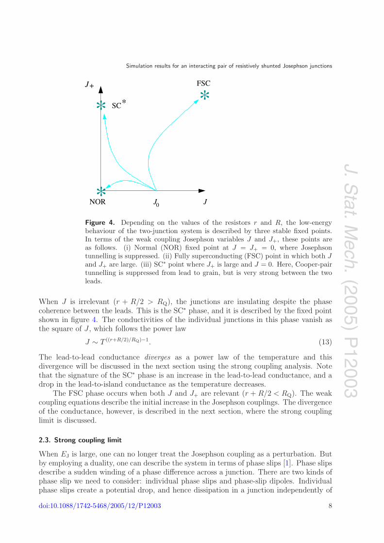
Figure 4. Depending on the values of the resistors r and R, the low-energybehaviour of the two-junction system is described by three stable fixed points.In terms of the weak coupling Josephson variables J and J+, these points areas follows. (i) Normal (NOR) fixed point at J = J+ = 0, where Josephsontunnelling is suppressed. (ii) Fully superconducting (FSC) point in which both Jand J+ are large. (iii) SC∗ point where J+ is large and J = 0. Here, Cooper-pairtunnelling is suppressed from lead to grain, but is very strong between the twoleads.

When J is irrelevant (r + R/2 > RQ), the junctions are insulating despite the phasecoherence between the leads. This is the SC∗ phase, and it is described by the fixed pointshown in figure 4. The conductivities of the individual junctions in this phase vanish asthe square of J , which follows the power law

J ∼ T ((r+R/2)/RQ)−1. (13)

The lead-to-lead conductance diverges as a power law of the temperature and thisdivergence will be discussed in the next section using the strong coupling analysis. Notethat the signature of the SC∗ phase is an increase in the lead-to-lead conductance, and adrop in the lead-to-island conductance as the temperature decreases.

The FSC phase occurs when both J and J+ are relevant (r + R/2 < RQ). The weakcoupling equations describe the initial increase in the Josephson couplings. The divergenceof the conductance, however, is described in the next section, where the strong couplinglimit is discussed.

2.3. Strong coupling limit

When EJ is large, one can no longer treat the Josephson coupling as a perturbation. Butby employing a duality, one can describe the system in terms of phase slips [1]. Phase slipsdescribe a sudden winding of a phase difference across a junction. There are two kinds ofphase slip we need to consider: individual phase slips and phase-slip dipoles. Individualphase slips create a potential drop, and hence dissipation in a junction independently of

doi:10.1088/1742-5468/2005/12/P12003 8

http://dx.doi.org/10.1088/1742-5468/2005/12/P12003

J.Stat.M

ech.(2005)

P12003


A B C

A B C

a.

b.

ζ

ζD

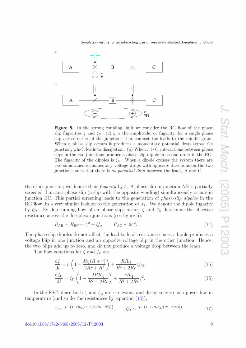
Figure 5. In the strong coupling limit we consider the RG flow of the phaseslip fugacities ζ and ζD. (a) ζ is the amplitude, or fugacity, for a single phaseslip across either of the junctions that connect the leads to the middle grain.When a phase slip occurs it produces a momentary potential drop across thejunction, which leads to dissipation. (b) When r > 0, interactions between phaseslips in the two junctions produce a phase-slip dipole in second order in the RG.The fugacity of the dipoles is ζD. When a dipole crosses the system there aretwo simultaneous momentary voltage drops with opposite directions on the twojunctions, such that there is no potential drop between the leads, A and C.

the other junction; we denote their fugacity by ζ . A phase slip in junction AB is partiallyscreened if an anti-phase slip (a slip with the opposite winding) simultaneously occurs injunction BC. This partial screening leads to the generation of phase-slip dipoles in theRG flow, in a very similar fashion to the generation of J+. We denote the dipole fugacityby ζD. By determining how often phase slips occur, ζ and ζD determine the effectiveresistance across the Josephson junctions (see figure 5):

RAB = RBC ∼ ζ2 + ζ2D, RAC ∼ 2ζ2. (14)

The phase-slip dipoles do not affect the lead-to-lead resistance since a dipole produces avoltage blip in one junction and an opposite voltage blip in the other junction. Hence,the two blips add up to zero, and do not produce a voltage drop between the leads.

The flow equations for ζ and ζD are

dζ

dl= ζ

(1 − RQ(R + r)

2Rr + R2

)+

RRQ

R2 + 2RrζζD, (15)

dζD

dl= ζD

(1 − 2RRQ

R2 + 2Rr

)+

rRQ

R2 + 2Rrζ2. (16)

In the FSC phase both ζ and ζD are irrelevant, and decay to zero as a power law intemperature (and so do the resistances by equation (14)),

ζ ∼ T−(1−(RQ(R+r)/(2Rr+R2))), ζD ∼ T−(1−(2RRQ/(R2+2Rr))). (17)

doi:10.1088/1742-5468/2005/12/P12003 9

http://dx.doi.org/10.1088/1742-5468/2005/12/P12003

J.Stat.M

ech.(2005)

P12003


SC*

ζ

ζζFSC

*NOR

*

*0

D

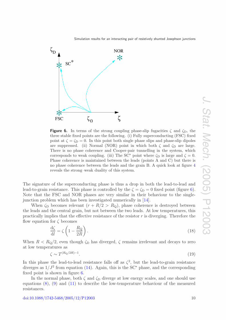
Figure 6. In terms of the strong coupling phase-slip fugacities ζ and ζD, thethree stable fixed points are the following. (i) Fully superconducting (FSC) fixedpoint at ζ = ζD = 0. In this point both single phase slips and phase-slip dipolesare suppressed. (ii) Normal (NOR) point in which both ζ and ζD are large.There is no phase coherence and Cooper-pair tunnelling in the system, whichcorresponds to weak coupling. (iii) The SC∗ point where ζD is large and ζ = 0.Phase coherence is maintained between the leads (points A and C) but there isno phase coherence between the leads and the grain B. A quick look at figure 4reveals the strong–weak duality of this system.

The signature of the superconducting phase is thus a drop in both the lead-to-lead andlead-to-grain resistance. This phase is controlled by the ζ = ζD = 0 fixed point (figure 6).Note that the FSC and NOR phases are very similar in their behaviour to the single-junction problem which has been investigated numerically in [14].

When ζD becomes relevant (r + R/2 > RQ), phase coherence is destroyed betweenthe leads and the central grain, but not between the two leads. At low temperatures, thispractically implies that the effective resistance of the resistor r is diverging. Therefore theflow equation for ζ becomes

dζ

dl= ζ

(1 − RQ

2R

). (18)

When R < RQ/2, even though ζD has diverged, ζ remains irrelevant and decays to zeroat low temperatures as

ζ ∼ T (RQ/2R)−1. (19)

In this phase the lead-to-lead resistance falls off as ζ2, but the lead-to-grain resistancediverges as 1/J2 from equation (14). Again, this is the SC∗ phase, and the correspondingfixed point is shown in figure 6.

In the normal phase, both ζ and ζD diverge at low energy scales, and one should useequations (8), (9) and (11) to describe the low-temperature behaviour of the measuredresistances.

doi:10.1088/1742-5468/2005/12/P12003 10

http://dx.doi.org/10.1088/1742-5468/2005/12/P12003

J.Stat.M

ech.(2005)

P12003


ζD

c

NOR

FSC

ζζ

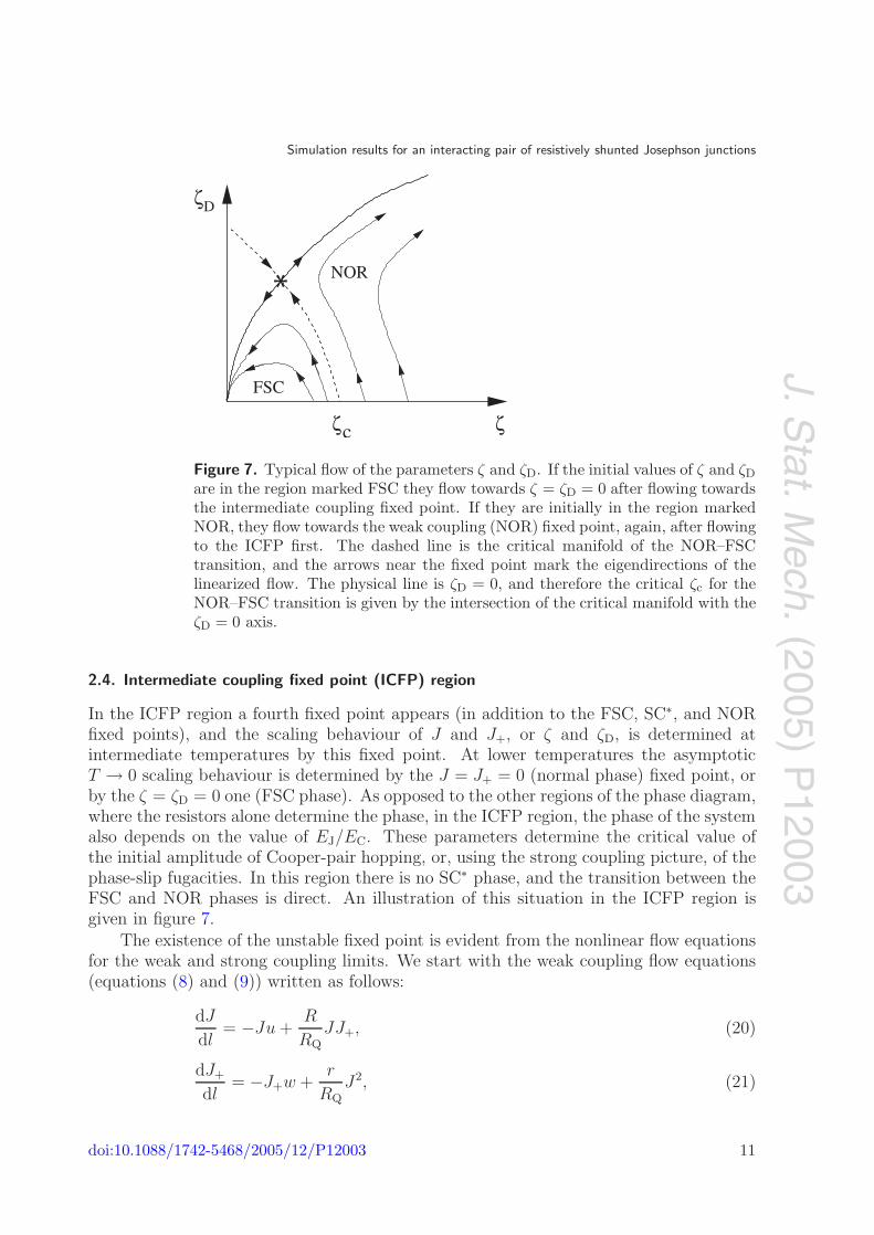
Figure 7. Typical flow of the parameters ζ and ζD. If the initial values of ζ and ζD

are in the region marked FSC they flow towards ζ = ζD = 0 after flowing towardsthe intermediate coupling fixed point. If they are initially in the region markedNOR, they flow towards the weak coupling (NOR) fixed point, again, after flowingto the ICFP first. The dashed line is the critical manifold of the NOR–FSCtransition, and the arrows near the fixed point mark the eigendirections of thelinearized flow. The physical line is ζD = 0, and therefore the critical ζc for theNOR–FSC transition is given by the intersection of the critical manifold with theζD = 0 axis.

2.4. Intermediate coupling fixed point (ICFP) region

In the ICFP region a fourth fixed point appears (in addition to the FSC, SC∗, and NORfixed points), and the scaling behaviour of J and J+, or ζ and ζD, is determined atintermediate temperatures by this fixed point. At lower temperatures the asymptoticT → 0 scaling behaviour is determined by the J = J+ = 0 (normal phase) fixed point, orby the ζ = ζD = 0 one (FSC phase). As opposed to the other regions of the phase diagram,where the resistors alone determine the phase, in the ICFP region, the phase of the systemalso depends on the value of EJ/EC. These parameters determine the critical value ofthe initial amplitude of Cooper-pair hopping, or, using the strong coupling picture, of thephase-slip fugacities. In this region there is no SC∗ phase, and the transition between theFSC and NOR phases is direct. An illustration of this situation in the ICFP region isgiven in figure 7.

The existence of the unstable fixed point is evident from the nonlinear flow equationsfor the weak and strong coupling limits. We start with the weak coupling flow equations(equations (8) and (9)) written as follows:

dJ

dl= −Ju +

R

RQJJ+, (20)

dJ+

dl= −J+w +

r

RQ

J2, (21)

doi:10.1088/1742-5468/2005/12/P12003 11

http://dx.doi.org/10.1088/1742-5468/2005/12/P12003

J.Stat.M

ech.(2005)

P12003


where

u =R + r

RQ− 1, w =

2R

RQ− 1. (22)

When both u > 0 and w > 0, the RG equations (20) and (21) have a third fixed point (inaddition to zero and ∞). This point is at

J∗ =RQ√rR

√uw, J∗

+ =RQ

Ru. (23)

Therefore the lines u = 0 and w = 0 mark the weak coupling boundaries of the ICFPregion (see figure 2).

Similarly, in the strong coupling limit we can write the flow equations (15) and (16)as

dζ

dl= −ζu +

RRQ

R2 + 2RrζζD, (24)

dζD

dl= −ζDv +

rRQ

R2 + 2Rrζ2, (25)

where

u =RQ(R + r)

2Rr + R2− 1, w =

2RRQ

R2 + 2Rr− 1. (26)

As in the weak coupling limit, when u > 0 and w > 0, an unstable fixed point appearsat intermediate values of ζ and ζD. The lines u > 0 and w > 0 mark the boundaries ofthe ICFP region on the strong coupling side. The fixed-point fugacities of the ICFP aregiven by

ζ∗ =R2 + 2rR

RQ

√rR

√uw, ζ∗

D =R2 + 2rR

RQRu. (27)

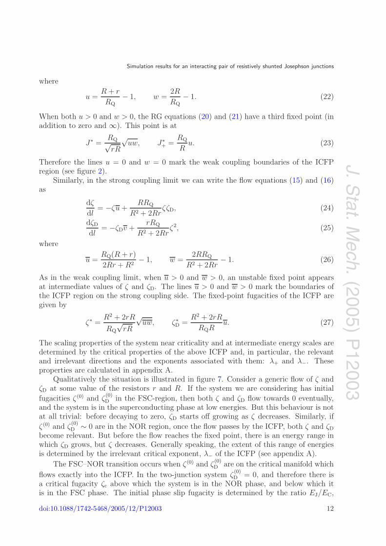
The scaling properties of the system near criticality and at intermediate energy scales aredetermined by the critical properties of the above ICFP and, in particular, the relevantand irrelevant directions and the exponents associated with them: λ+ and λ−. Theseproperties are calculated in appendix A.

Qualitatively the situation is illustrated in figure 7. Consider a generic flow of ζ andζD at some value of the resistors r and R. If the system we are considering has initial

fugacities ζ (0) and ζ(0)D in the FSC-region, then both ζ and ζD flow towards 0 eventually,

and the system is in the superconducting phase at low energies. But this behaviour is notat all trivial: before decaying to zero, ζD starts off growing as ζ decreases. Similarly, if

ζ (0) and ζ(0)D ∼ 0 are in the NOR region, once the flow passes by the ICFP, both ζ and ζD

become relevant. But before the flow reaches the fixed point, there is an energy range inwhich ζD grows, but ζ decreases. Generally speaking, the extent of this range of energiesis determined by the irrelevant critical exponent, λ− of the ICFP (see appendix A).

The FSC–NOR transition occurs when ζ (0) and ζ(0)D are on the critical manifold which

flows exactly into the ICFP. In the two-junction system ζ(0)D = 0, and therefore there is

a critical fugacity ζc above which the system is in the NOR phase, and below which itis in the FSC phase. The initial phase slip fugacity is determined by the ratio EJ/EC,

doi:10.1088/1742-5468/2005/12/P12003 12

http://dx.doi.org/10.1088/1742-5468/2005/12/P12003

J.Stat.M

ech.(2005)

P12003


and therefore this transition (for a given value of the resistances R and r in the ICFPregion) can be tuned by changing the Josephson energy. The qualitative picture describedabove is equally valid in weak coupling, where the only difference would be discussing thepair-tunnelling amplitudes, J and J+, rather than the phase-slip fugacities.

The flow of the fugacities (or pair tunnelling amplitudes) before reaching the ICFPdetermines the behaviour of the resistance as a function of temperature at intermediatetemperatures. In these temperature ranges the behaviour of the resistance may bemisinterpreted as any of the three phases of the system. Particularly, in the region ofparameter space where ζ decreases and ζD increases, the lead-to-lead resistance decreases,since it is only proportional to ζ2, but the lead-to-grain resistance increases. Thisbehaviour could be misinterpreted as the system being in the SC∗ phase. In order todetermine the true T = 0 phase one has to investigate the system at very low temperatures.These crossover effects indeed appear explicitly in the Monte Carlo simulations of thesystem.

3. Monte Carlo method

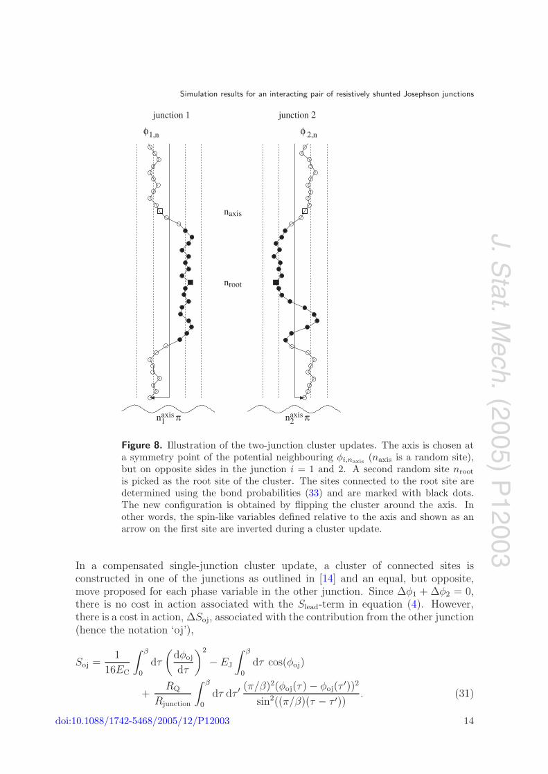
Monte Carlo simulations of the two-junction model as shown in the lower part of figure 1can be performed using variants of the local and cluster updates detailed in [14]. Imaginarytime is divided into N time slices of size ∆τ = β/N and the variables φ1,n and φ2,n,n = 1, . . . , N (phase differences across the junctions at the discrete times τn = n∆τ) areused to represent the phase configuration (see figure 8). We implemented the followingtypes of Monte Carlo updates.

(1) Single-junction cluster updatesA cluster of connected sites is constructed in one of the junctions as outlined in [14].The cost in action of flipping the cluster, ∆Slead, which is associated with the lastterm in equation (4),

Slead =RQ

Rlead

∫ β

0

dτ dτ ′ (π/β)2

sin2((π/β)(τ − τ ′))

× ((φ1(τ) + φ2(τ)) − (φ1(τ′) + φ2(τ

′)))2, (28)

must be calculated and the cluster move accepted with probability

p = min(1, exp(−∆Slead)). (29)

(2) Single-junction local updatesLocal updates in Fourier space are proposed in one of the junction, as detailed in [14].They, too, are accepted with probability


(3) Compensated single-junction cluster updatesThe SC∗-phase is characterized by phase coherence between the leads (φ1(τ) +φ2(τ) ≈ constant) but strong fluctuations of the variables φ1(τ) and φ2(τ) (insulatingjunctions). Therefore, the fluctuations in the two junctions essentially compensateeach other and efficient updates in the SC∗-phase should take this constraint intoaccount.

doi:10.1088/1742-5468/2005/12/P12003 13

http://dx.doi.org/10.1088/1742-5468/2005/12/P12003

J.Stat.M

ech.(2005)

P12003


π

junction 1 junction 2

φ φ1,n 2,n

axisn

nroot

axisn1 π n2axis

Figure 8. Illustration of the two-junction cluster updates. The axis is chosen ata symmetry point of the potential neighbouring φi,naxis

(naxis is a random site),but on opposite sides in the junction i = 1 and 2. A second random site nroot

is picked as the root site of the cluster. The sites connected to the root site aredetermined using the bond probabilities (33) and are marked with black dots.The new configuration is obtained by flipping the cluster around the axis. Inother words, the spin-like variables defined relative to the axis and shown as anarrow on the first site are inverted during a cluster update.

In a compensated single-junction cluster update, a cluster of connected sites isconstructed in one of the junctions as outlined in [14] and an equal, but opposite,move proposed for each phase variable in the other junction. Since ∆φ1 + ∆φ2 = 0,there is no cost in action associated with the Slead-term in equation (4). However,there is a cost in action, ∆Soj, associated with the contribution from the other junction(hence the notation ‘oj’),

Soj =1

16EC

∫ β

0

dτ

(dφoj

dτ

)2

− EJ

∫ β

0

dτ cos(φoj)

+RQ

Rjunction

∫ β

0

dτ dτ ′ (π/β)2(φoj(τ) − φoj(τ′))2

sin2((π/β)(τ − τ ′)). (31)

doi:10.1088/1742-5468/2005/12/P12003 14

http://dx.doi.org/10.1088/1742-5468/2005/12/P12003

J.Stat.M

ech.(2005)

P12003


The compensated cluster move should therefore be accepted with probability

p = min(1, exp(−∆Soj)). (32)

(4) Two-junction cluster updatesA random site k is picked and an axis ni in each of the two junctions chosen amongthe two closest to φi(τk), such that n1π ≤ φ1,k and n2π ≥ φ2,k or vice versa (seefigure 8). Relative coordinates φaxis

i = φi − naxisi π are introduced in both junctions

and a cluster of sites connected to a randomly chosen root site is constructed usingthe bond probabilities

p(k, l) = max(0, 1 − exp(−∆Sk,l)) (33)

where the cost in action of breaking a bond, ∆Sk,l, is defined as

∆Sk,l =∑i=1,2

(S(φaxis

i,k ,−φaxisi,l ) − S(φaxis

i,k , φaxisi,l )

)

= 8g(k − l)∑i=1,2

φaxisi,k φaxis

i,l . (34)

In the above expression, g(j) is the kernel (j = 0)

g(j) =1

32EC∆τ(δj,1 + δj,N−1) +

1

8π2

RQ

Rjunction

(π/N)2

sin((π/N)j)2. (35)

Hence, in contrast to the single-junction case, a cluster can contain relative phasevariables of both signs. The cluster building process (34) takes into account thecapacitive, dissipative and Josephson contributions from both junctions, but not thedissipative contribution from the Slead-term. A two-junction cluster move thereforecan only be accepted with probability


4. Phase diagram

We first use the efficient Monte Carlo scheme outlined in section 3 to identify the threephases NOR, FSC and SC∗, and to determine the phase diagram for an intermediate valueof the Josephson coupling EJ. This allows us to test the theoretical predictions outlinedin section 2 and in figure 2.

The result of this study is shown in figure 11 and explained in section 4.1. Theagreement between the Monte Carlo calculation and the theory is very good. Smalldeviations, however, appear in the vicinity of the (tricritical) meeting point of the threephases: r = 0.75RQ and R = RQ/2. These deviations from the theoretically predictedphase diagram are explained in section 4.2 as crossover effects, and are indirect evidencefor the existence of the intermediate coupling fixed point.

4.1. Simulation results

We use the resistance at imaginary frequencies to identify the state of conductance betweenthe leads and from the leads to the central grain. The imaginary frequency resistance is

doi:10.1088/1742-5468/2005/12/P12003 15

http://dx.doi.org/10.1088/1742-5468/2005/12/P12003

J.Stat.M

ech.(2005)

P12003


0

0.2

0.4

0.6

0.8

1

0 0.05 0.1 0.15 0.2 0.25 0.3 0.35

R(ω

n)/

RQ

ωn / EC

r / RQ=0.5 lead-grain

0

0.2

0.4

0.6

0.8

1

0 0.05 0.1 0.15 0.2 0.25 0.3 0.35

R(ω

n)/

RQ

ωn / EC

r / RQ=0.5 lead-lead

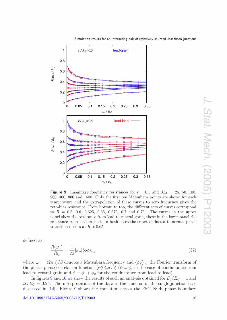
Figure 9. Imaginary frequency resistances for r = 0.5 and βEC = 25, 50, 100,200, 400, 800 and 1600. Only the first ten Matsubara points are shown for eachtemperature and the extrapolation of these curves to zero frequency gives thezero-bias resistance. From bottom to top, the different sets of curves correspondto R = 0.5, 0.6, 0.625, 0.65, 0.675, 0.7 and 0.75. The curves in the upperpanel show the resistance from lead to central grain, those in the lower panel theresistance from lead to lead. In both cases the superconductor-to-normal phasetransition occurs at R ≈ 0.65.

defined as

R(ωn)

RQ=

1

2π|ωn|〈φφ〉ωn, (37)

where ωn = (2πn)/β denotes a Matsubara frequency and 〈φφ〉ωn the Fourier transform ofthe phase–phase correlation function 〈φ(0)φ(τ)〉 (φ ≡ φi in the case of conductance fromlead to central grain and φ ≡ φ1 + φ2 for the conductance from lead to lead).

In figures 9 and 10 we show the results of such an analysis obtained for EJ/EC = 1 and∆τEC = 0.25. The interpretation of the data is the same as in the single-junction casediscussed in [14]. Figure 9 shows the transition across the FSC–NOR phase boundary

doi:10.1088/1742-5468/2005/12/P12003 16

http://dx.doi.org/10.1088/1742-5468/2005/12/P12003

J.Stat.M

ech.(2005)

P12003


0

0.2

0.4

0.6

0.8

1

1.2

1.4

0 0.05 0.1 0.15 0.2 0.25 0.3 0.35

R(ω

n)/

RQ

ωn / EC

r / RQ=1.1 lead-grain

0

0.2

0.4

0.6

0.8

1

1.2

1.4

0 0.05 0.1 0.15 0.2 0.25 0.3 0.35

R(ω

n)/

RQ

ωn / EC

r / RQ=1.1 lead-lead

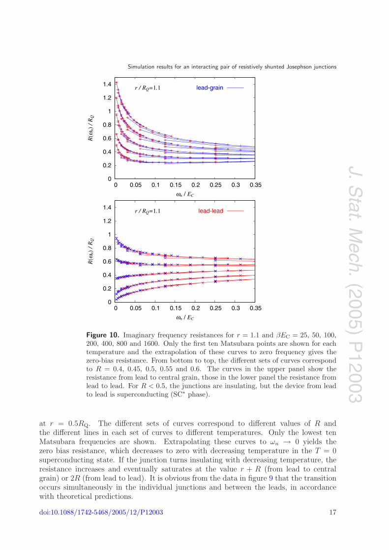
Figure 10. Imaginary frequency resistances for r = 1.1 and βEC = 25, 50, 100,200, 400, 800 and 1600. Only the first ten Matsubara points are shown for eachtemperature and the extrapolation of these curves to zero frequency gives thezero-bias resistance. From bottom to top, the different sets of curves correspondto R = 0.4, 0.45, 0.5, 0.55 and 0.6. The curves in the upper panel show theresistance from lead to central grain, those in the lower panel the resistance fromlead to lead. For R < 0.5, the junctions are insulating, but the device from leadto lead is superconducting (SC∗ phase).

at r = 0.5RQ. The different sets of curves correspond to different values of R andthe different lines in each set of curves to different temperatures. Only the lowest tenMatsubara frequencies are shown. Extrapolating these curves to ωn → 0 yields thezero bias resistance, which decreases to zero with decreasing temperature in the T = 0superconducting state. If the junction turns insulating with decreasing temperature, theresistance increases and eventually saturates at the value r + R (from lead to centralgrain) or 2R (from lead to lead). It is obvious from the data in figure 9 that the transitionoccurs simultaneously in the individual junctions and between the leads, in accordancewith theoretical predictions.

doi:10.1088/1742-5468/2005/12/P12003 17

http://dx.doi.org/10.1088/1742-5468/2005/12/P12003

J.Stat.M

ech.(2005)

P12003


0

0.2

0.4

0.6

0.8

1

1.2

1.4

0 0.2 0.4 0.6 0.8 1 1.2

r / R

QSC*

SC

N

junction insulatingjunction supra

junction criticalleads insulating

leads supraleads critical

R / RQ

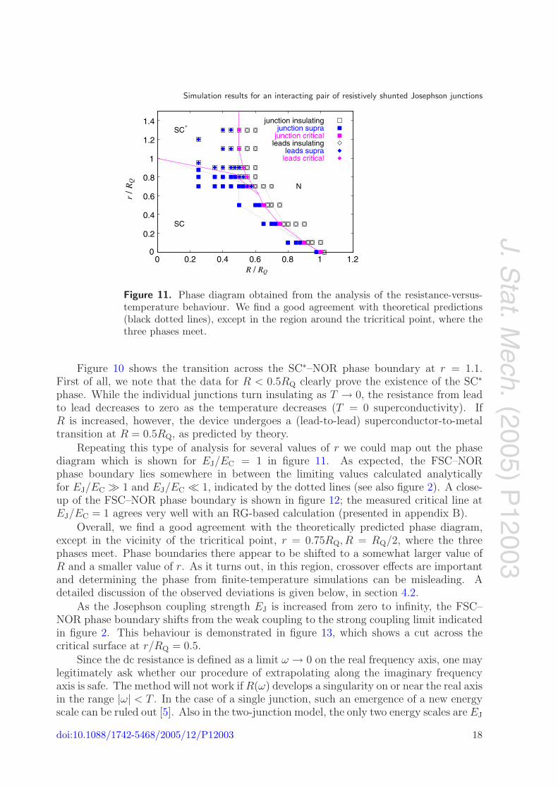
Figure 11. Phase diagram obtained from the analysis of the resistance-versus-temperature behaviour. We find a good agreement with theoretical predictions(black dotted lines), except in the region around the tricritical point, where thethree phases meet.

Figure 10 shows the transition across the SC∗–NOR phase boundary at r = 1.1.First of all, we note that the data for R < 0.5RQ clearly prove the existence of the SC∗

phase. While the individual junctions turn insulating as T → 0, the resistance from leadto lead decreases to zero as the temperature decreases (T = 0 superconductivity). IfR is increased, however, the device undergoes a (lead-to-lead) superconductor-to-metaltransition at R = 0.5RQ, as predicted by theory.

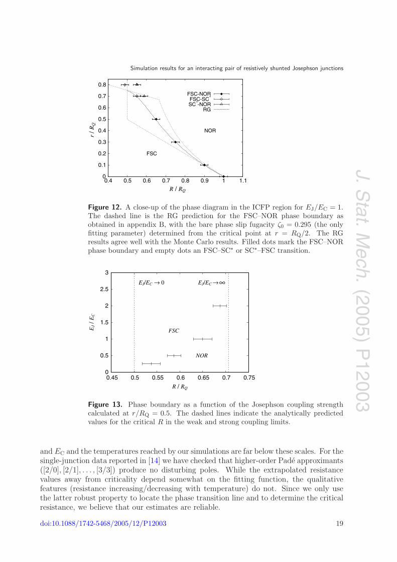
Repeating this type of analysis for several values of r we could map out the phasediagram which is shown for EJ/EC = 1 in figure 11. As expected, the FSC–NORphase boundary lies somewhere in between the limiting values calculated analyticallyfor EJ/EC 1 and EJ/EC 1, indicated by the dotted lines (see also figure 2). A close-up of the FSC–NOR phase boundary is shown in figure 12; the measured critical line atEJ/EC = 1 agrees very well with an RG-based calculation (presented in appendix B).

Overall, we find a good agreement with the theoretically predicted phase diagram,except in the vicinity of the tricritical point, r = 0.75RQ, R = RQ/2, where the threephases meet. Phase boundaries there appear to be shifted to a somewhat larger value ofR and a smaller value of r. As it turns out, in this region, crossover effects are importantand determining the phase from finite-temperature simulations can be misleading. Adetailed discussion of the observed deviations is given below, in section 4.2.

As the Josephson coupling strength EJ is increased from zero to infinity, the FSC–NOR phase boundary shifts from the weak coupling to the strong coupling limit indicatedin figure 2. This behaviour is demonstrated in figure 13, which shows a cut across thecritical surface at r/RQ = 0.5.

Since the dc resistance is defined as a limit ω → 0 on the real frequency axis, one maylegitimately ask whether our procedure of extrapolating along the imaginary frequencyaxis is safe. The method will not work if R(ω) develops a singularity on or near the real axisin the range |ω| < T . In the case of a single junction, such an emergence of a new energyscale can be ruled out [5]. Also in the two-junction model, the only two energy scales are EJ

doi:10.1088/1742-5468/2005/12/P12003 18

http://dx.doi.org/10.1088/1742-5468/2005/12/P12003

J.Stat.M

ech.(2005)

P12003


0

0.1

0.2

0.3

0.4

0.5

0.6

0.7

0.8

0.4 0.5 0.6 0.7 0.8 0.9 1 1.1

r / R

Q

R / RQ

FSC

NOR

FSC-NORFSC-SC*

SC*-NORRG

Figure 12. A close-up of the phase diagram in the ICFP region for EJ/EC = 1.The dashed line is the RG prediction for the FSC–NOR phase boundary asobtained in appendix B, with the bare phase slip fugacity ζ0 = 0.295 (the onlyfitting parameter) determined from the critical point at r = RQ/2. The RGresults agree well with the Monte Carlo results. Filled dots mark the FSC–NORphase boundary and empty dots an FSC–SC∗ or SC∗–FSC transition.

0

0.5

1

1.5

2

2.5

3

0.45 0.5 0.55 0.6 0.65 0.7 0.75

EJ

/ EC

R / RQ

EJ/EC 0 EJ/EC

FSC

NOR

Figure 13. Phase boundary as a function of the Josephson coupling strengthcalculated at r/RQ = 0.5. The dashed lines indicate the analytically predictedvalues for the critical R in the weak and strong coupling limits.

and EC and the temperatures reached by our simulations are far below these scales. For thesingle-junction data reported in [14] we have checked that higher-order Pade approximants([2/0], [2/1], . . . , [3/3]) produce no disturbing poles. While the extrapolated resistancevalues away from criticality depend somewhat on the fitting function, the qualitativefeatures (resistance increasing/decreasing with temperature) do not. Since we only usethe latter robust property to locate the phase transition line and to determine the criticalresistance, we believe that our estimates are reliable.

doi:10.1088/1742-5468/2005/12/P12003 19

http://dx.doi.org/10.1088/1742-5468/2005/12/P12003

J.Stat.M

ech.(2005)

P12003


Of course, any extrapolation of numerical data will fail if a crossover occurs at aninaccessibly low temperature. The implications of this for the interpretation of figure 11will be discussed in the following section.

4.2. Crossover effects in the Monte Carlo results

The theory of the two-junction system as outlined in section 2 and in appendix A leadsus to expect crossover behaviour at intermediate temperatures. Although the rangeof temperatures at our disposal is limited, and the crossover regime spans a narrowrange of energy scales, we see indirect evidence of the crossover effects in the measuredphase diagram. As mentioned above, near the meeting point of the three phases, thepredicted phase boundaries do not completely agree with the Monte Carlo simulationresults (figure 11). We will explain these deviations using the RG analysis.

The deviations of the measured data from the theoretical predictions can beunderstood by looking at the RG trajectories given by equations (15) and (16). Asexplained in section 2.4, the flow of the phase slip fugacities or pair-tunnelling amplitudesnear the intermediate coupling fixed point can make the measured resistance as a functionof temperature behave as though the system is in the SC∗ phase. Near the meeting pointof the three phases, the flow towards the ICFP is extremely slow; it is dominated by thecritical exponent λ− given by equations (A.9) and (A.22):

λ(weak)− = 1

2

(−w −

√w2 + 8uw

), (38)

λ(strong)− = 1

2

(−w −

√w2 + 8uw

), (39)

where u, w and u, w are defined in equations (22) and (26). More specifically, in thisregime x−x∗ ∼ T λ− with x being ζ , ζD, or J , J+, and x∗ the respective fixed-point value.As can be seen from equations (38), (39) and figure 2, λ− in both the weak and strongcoupling regimes vanishes at the meeting point (w = w = 0), and therefore is expectedto be small near this special point for any value of the Josephson coupling. This impliesthat since the Monte Carlo calculation is limited to temperatures above T = Ec/2500 (ifwe choose ∆τEC = 0.25, which seems appropriate) it may not probe the ground stateof the system, but rather the crossover physics. This will lead to distorted NOR–FSCphase boundaries in this region. As it turns out, this phenomenon is not restricted to theICFP region: slow crossovers occur all around the triple point and may shift the observedNOR–SC∗ and SC∗–FSC phase boundaries, as indeed is seen in figure 11.

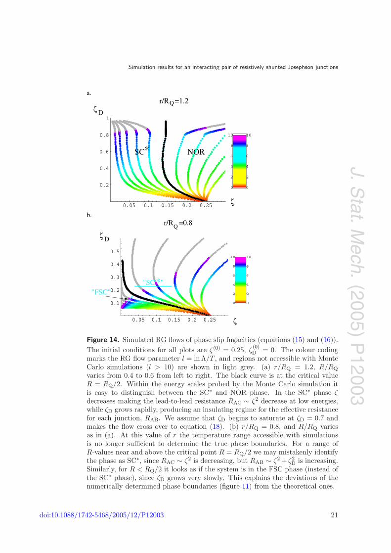
To demonstrate the above behaviour we plot the predicted RG flow of the phase slipfugacities in the strong coupling limit for four values of r/RQ in the region of interest(figures 14 and 15). We colour coded the plot according to the RG flow parameterl = ln Λ/T where Λ is the ultraviolet cutoff. Roughly speaking, the maximum RG scalewe probe in the Monte Carlo calculation is lmax ≈ 7, and therefore we stop the colourcoding at the value l = 10. The various flow lines all start with the same initial fugacity(same EJ/EC), but have the resistance R varied across the transition. In the Monte Carlosimulation one measures the lead-to-lead resistance, which we expect to behave as

RAC ∼ ζ2, (40)

doi:10.1088/1742-5468/2005/12/P12003 20

http://dx.doi.org/10.1088/1742-5468/2005/12/P12003

J.Stat.M

ech.(2005)

P12003


0.05 0.1 0.15 0.2 0.25

0.2

0.4

0.6

0.8

1

0

2

4

6

8

10

0

2

4

6

8

10

ζ D

ζ

SC* NOR

a.r/R =1.2Q

0.05 0.1 0.15 0.2 0.25

0.1

0.2

0.3

0.4

0.5

0

2

4

6

8

10

0

2

4

6

8

10

ζ D

ζ

"SC "*"FSC"

Q

b.r/R =0.8

Figure 14. Simulated RG flows of phase slip fugacities (equations (15) and (16)).The initial conditions for all plots are ζ(0) = 0.25, ζ

(0)D = 0. The colour coding

marks the RG flow parameter l = ln Λ/T , and regions not accessible with MonteCarlo simulations (l > 10) are shown in light grey. (a) r/RQ = 1.2, R/RQ

varies from 0.4 to 0.6 from left to right. The black curve is at the critical valueR = RQ/2. Within the energy scales probed by the Monte Carlo simulation itis easy to distinguish between the SC∗ and NOR phase. In the SC∗ phase ζdecreases making the lead-to-lead resistance RAC ∼ ζ2 decrease at low energies,while ζD grows rapidly, producing an insulating regime for the effective resistancefor each junction, RAB. We assume that ζD begins to saturate at ζD = 0.7 andmakes the flow cross over to equation (18). (b) r/RQ = 0.8, and R/RQ variesas in (a). At this value of r the temperature range accessible with simulationsis no longer sufficient to determine the true phase boundaries. For a range ofR-values near and above the critical point R = RQ/2 we may mistakenly identifythe phase as SC∗, since RAC ∼ ζ2 is decreasing, but RAB ∼ ζ2 + ζ2

D is increasing.Similarly, for R < RQ/2 it looks as if the system is in the FSC phase (instead ofthe SC∗ phase), since ζD grows very slowly. This explains the deviations of thenumerically determined phase boundaries (figure 11) from the theoretical ones.

doi:10.1088/1742-5468/2005/12/P12003 21

http://dx.doi.org/10.1088/1742-5468/2005/12/P12003

J.Stat.M

ech.(2005)

P12003


0.05 0.1 0.15 0.2 0.25

0.05

0.1

0.15

0.2

0.25

0.3

0

2

4

6

8

10

0

2

4

6

8

10

ζ D

ζ

*"SC "

c. r/R =0.7Q

0.1 0.2 0.3 0.4

0.025

0.05

0.075

0.1

0.125

0.15

0

2

4

6

8

10

0

2

4

6

8

10

ζ D

NOR

ζ

d.r/R =0.5Q

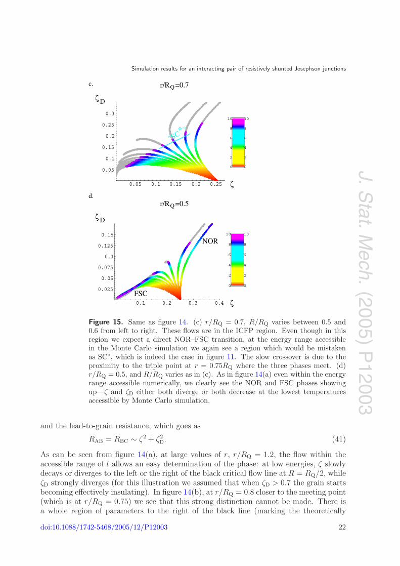
FSC

Figure 15. Same as figure 14. (c) r/RQ = 0.7, R/RQ varies between 0.5 and0.6 from left to right. These flows are in the ICFP region. Even though in thisregion we expect a direct NOR–FSC transition, at the energy range accessiblein the Monte Carlo simulation we again see a region which would be mistakenas SC∗, which is indeed the case in figure 11. The slow crossover is due to theproximity to the triple point at r = 0.75RQ where the three phases meet. (d)r/RQ = 0.5, and R/RQ varies as in (c). As in figure 14(a) even within the energyrange accessible numerically, we clearly see the NOR and FSC phases showingup—ζ and ζD either both diverge or both decrease at the lowest temperaturesaccessible by Monte Carlo simulation.

and the lead-to-grain resistance, which goes as

RAB = RBC ∼ ζ2 + ζ2D. (41)

As can be seen from figure 14(a), at large values of r, r/RQ = 1.2, the flow within theaccessible range of l allows an easy determination of the phase: at low energies, ζ slowlydecays or diverges to the left or the right of the black critical flow line at R = RQ/2, whileζD strongly diverges (for this illustration we assumed that when ζD > 0.7 the grain startsbecoming effectively insulating). In figure 14(b), at r/RQ = 0.8 closer to the meeting point(which is at r/RQ = 0.75) we see that this strong distinction cannot be made. There isa whole region of parameters to the right of the black line (marking the theoretically

doi:10.1088/1742-5468/2005/12/P12003 22

http://dx.doi.org/10.1088/1742-5468/2005/12/P12003

J.Stat.M

ech.(2005)

P12003


predicted critical flow), in which the lead-to-lead resistance (RAC ∼ ζ2) decreases, andthe single-junction resistance (RAB ∼ ζ2 + ζ2

D) increases. This region eventually flows tothe normal fixed point, but in the finite-temperature Monte Carlo simulations this cannotbe observed and it appears that an SC∗ phase exists at values R > RQ/2, as shown infigure 11. To the left of the black line in figure 14(b) we theoretically expect the SC∗

phase, but even there we see a crossover which will be misinterpreted as an FSC phase:RAB decreases and, for a range of parameters, also RAC. RAC only starts to grow at alower energy scale, disclosing the true SC∗ phase. Indeed, in figure 11 we see that theMonte Carlo calculation indicates an FSC region at r/RQ = 0.8 and R < 0.5RQ, where itshould be the SC∗ phase.

In the ICFP region we again encounter slow crossovers associated with theintermediate coupling fixed point. As can be seen in figure 15(c) with r/RQ = 0.7,there is a range of parameters which would be mistaken for the SC∗ phase, in which RAC

seems to drop, while RAB grows. Since the RG is stopped approximately at the lmax

corresponding to our Monte Carlo calculation, the observed flow in this case is dominatedonly by the critical exponent λ− of equations (38) and (39), which vanishes at the triplepoint. For comparison, in figure 15(d) we show the RG flow for r/RQ = 0.5. In this casethe RG does flow to the stable NOR and FSC fixed points at energy scales higher than thelowest temperature accessible in our calculation. Indeed, in this parameter range there isno longer any evidence of an SC∗-like phase in the Monte Carlo calculation.

5. The critical two-junction system in the ICFP region—comparison with a singleJosephson junction

In this section we investigate the direct NOR–FSC transition, and compare the criticalbehaviour of the two-junction system with that of a single junction with the sameEJ/EC. We make a rather surprising observation: along this phase boundary, the effectiveresistance of the junction, the temperature dependence of the mean phase fluctuations,and the correlation exponents are within error-bars the same as those in a single resistivelyshunted Josephson junction at criticality (with the same EJ/EC and ∆τEC). This suggeststhat many of the features of the NOR–FSC transition at the ICFP can be understood interms of the single-junction Schmid transition, although the ICFP is an interacting fixedpoint. We will first present the numerical results and then proceed to discuss them insections 5.2 and 6.

5.1. Numerical results and resemblance to the single junction

Associated with the drift of the phase boundary in the ICFP region as a function of EJ/EC

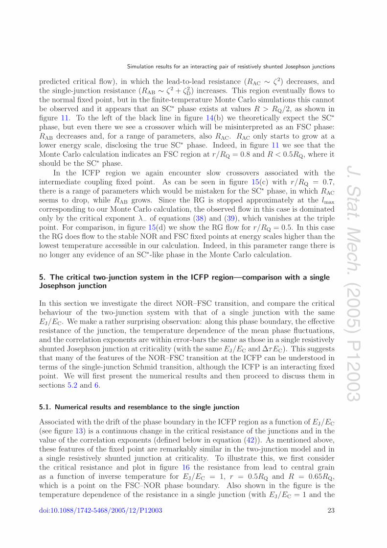
(see figure 13) is a continuous change in the critical resistance of the junctions and in thevalue of the correlation exponents (defined below in equation (42)). As mentioned above,these features of the fixed point are remarkably similar in the two-junction model and ina single resistively shunted junction at criticality. To illustrate this, we first considerthe critical resistance and plot in figure 16 the resistance from lead to central grainas a function of inverse temperature for EJ/EC = 1, r = 0.5RQ and R = 0.65RQ,which is a point on the FSC–NOR phase boundary. Also shown in the figure is thetemperature dependence of the resistance in a single junction (with EJ/EC = 1 and the

doi:10.1088/1742-5468/2005/12/P12003 23

http://dx.doi.org/10.1088/1742-5468/2005/12/P12003

J.Stat.M

ech.(2005)

P12003


0.1

1

100 1000 10000

R /

RQ

4βEC

single junctiontwo-junction system

Figure 16. Critical lead-to-grain resistance as a function of inverse temperaturefor EJ/EC = 1 and ∆τEC = 0.25. The point r = 0.5RQ, R = 0.65RQ on theFSC–NOR phase boundary has been selected (see figure 11). For comparison,we also plot resistance-versus-temperature data for a single resistively shuntedjunction with EJ/EC = 1 and ∆τEC = 0.25. The values Rs of the shunt resistorsare (from top to bottom) RQ/Rs = 0.9, 0.95, 0.975, 1.0, 1.025, 1.05, and 1.1,respectively. At the phase transition point RQ/Rs = 1, the resistance of thesingle junction is exactly the same as the critical lead-to-grain resistance in thetwo-junction system.

same discretization step ∆τEC = 0.25) for several values of the shunt resistance Rs. Thecurves from top to bottom correspond to RQ/Rs = 0.9, 0.95, 0.975, 1.0, 1.025, 1.05 and1.1, respectively. For RQ/Rs > 1, the junction turns superconducting as T → 0, whereasfor RQ/Rs < 1 it becomes insulating. At the critical point RQ/Rs = 1, the resistance ofthe system (junction plus shunt resistor) is precisely the same as the critical resistancefrom lead to central grain in the two-junction model.

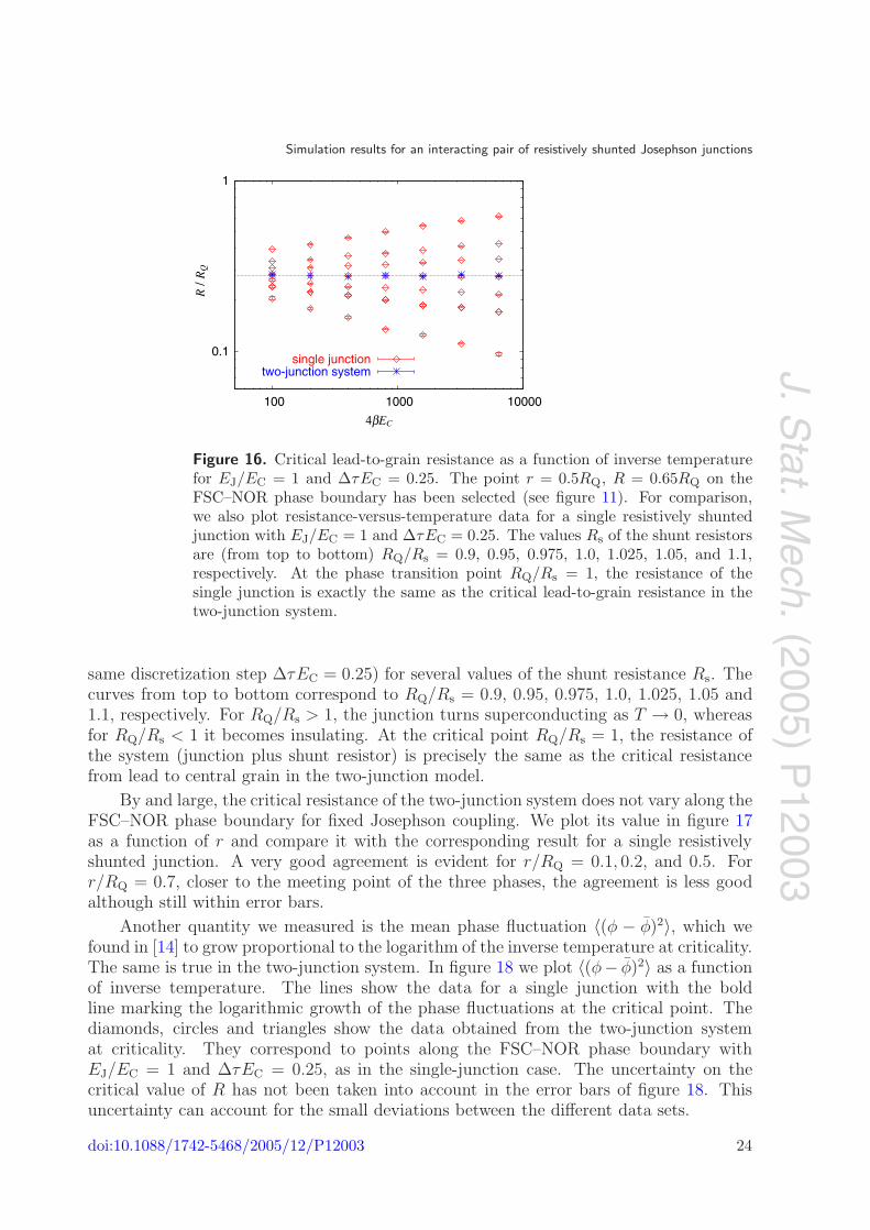
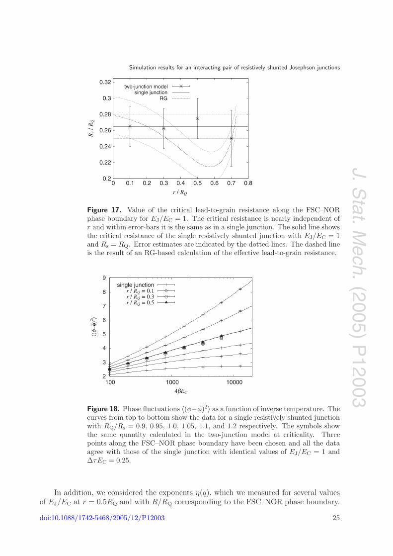
By and large, the critical resistance of the two-junction system does not vary along theFSC–NOR phase boundary for fixed Josephson coupling. We plot its value in figure 17as a function of r and compare it with the corresponding result for a single resistivelyshunted junction. A very good agreement is evident for r/RQ = 0.1, 0.2, and 0.5. Forr/RQ = 0.7, closer to the meeting point of the three phases, the agreement is less goodalthough still within error bars.

Another quantity we measured is the mean phase fluctuation 〈(φ − φ)2〉, which wefound in [14] to grow proportional to the logarithm of the inverse temperature at criticality.The same is true in the two-junction system. In figure 18 we plot 〈(φ− φ)2〉 as a functionof inverse temperature. The lines show the data for a single junction with the boldline marking the logarithmic growth of the phase fluctuations at the critical point. Thediamonds, circles and triangles show the data obtained from the two-junction systemat criticality. They correspond to points along the FSC–NOR phase boundary withEJ/EC = 1 and ∆τEC = 0.25, as in the single-junction case. The uncertainty on thecritical value of R has not been taken into account in the error bars of figure 18. Thisuncertainty can account for the small deviations between the different data sets.

doi:10.1088/1742-5468/2005/12/P12003 24

http://dx.doi.org/10.1088/1742-5468/2005/12/P12003

J.Stat.M

ech.(2005)

P12003


0.2

0.22

0.24

0.26

0.28

0.3

0.32

0 0.1 0.2 0.3 0.4 0.5 0.6 0.7 0.8

Rc

/ RQ

r / RQ

two-junction modelsingle junction

RG

Figure 17. Value of the critical lead-to-grain resistance along the FSC–NORphase boundary for EJ/EC = 1. The critical resistance is nearly independent ofr and within error-bars it is the same as in a single junction. The solid line showsthe critical resistance of the single resistively shunted junction with EJ/EC = 1and Rs = RQ. Error estimates are indicated by the dotted lines. The dashed lineis the result of an RG-based calculation of the effective lead-to-grain resistance.

2

3

4

5

6

7

8

9

100 1000 10000

4β EC

single junctionr / RQ = 0.1r / RQ = 0.3r / RQ = 0.5

⟨(φ−

φ– )2 ⟩

Figure 18. Phase fluctuations 〈(φ−φ)2〉 as a function of inverse temperature. Thecurves from top to bottom show the data for a single resistively shunted junctionwith RQ/Rs = 0.9, 0.95, 1.0, 1.05, 1.1, and 1.2 respectively. The symbols showthe same quantity calculated in the two-junction model at criticality. Threepoints along the FSC–NOR phase boundary have been chosen and all the dataagree with those of the single junction with identical values of EJ/EC = 1 and∆τEC = 0.25.

In addition, we considered the exponents η(q), which we measured for several valuesof EJ/EC at r = 0.5RQ and with R/RQ corresponding to the FSC–NOR phase boundary.

doi:10.1088/1742-5468/2005/12/P12003 25

http://dx.doi.org/10.1088/1742-5468/2005/12/P12003

J.Stat.M

ech.(2005)

P12003


0.1

1

1 10 100 1000 10000

exp(

i/4(

φ τ−φ

0))

4τEC

EJ /EC

2

1

0.5

0.25two junctions

single junction

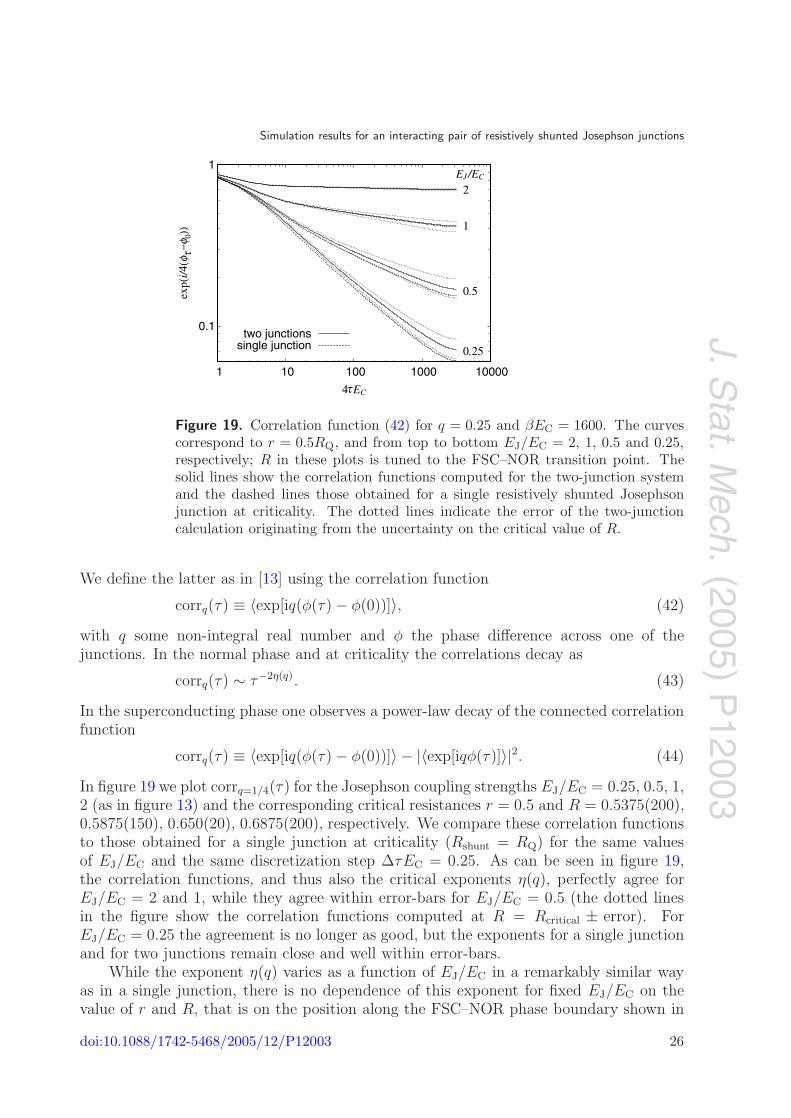
Figure 19. Correlation function (42) for q = 0.25 and βEC = 1600. The curvescorrespond to r = 0.5RQ, and from top to bottom EJ/EC = 2, 1, 0.5 and 0.25,respectively; R in these plots is tuned to the FSC–NOR transition point. Thesolid lines show the correlation functions computed for the two-junction systemand the dashed lines those obtained for a single resistively shunted Josephsonjunction at criticality. The dotted lines indicate the error of the two-junctioncalculation originating from the uncertainty on the critical value of R.

We define the latter as in [13] using the correlation function

corrq(τ) ≡ 〈exp[iq(φ(τ) − φ(0))]〉, (42)

with q some non-integral real number and φ the phase difference across one of thejunctions. In the normal phase and at criticality the correlations decay as

corrq(τ) ∼ τ−2η(q). (43)

In the superconducting phase one observes a power-law decay of the connected correlationfunction

corrq(τ) ≡ 〈exp[iq(φ(τ) − φ(0))]〉 − |〈exp[iqφ(τ)]〉|2. (44)

In figure 19 we plot corrq=1/4(τ) for the Josephson coupling strengths EJ/EC = 0.25, 0.5, 1,2 (as in figure 13) and the corresponding critical resistances r = 0.5 and R = 0.5375(200),0.5875(150), 0.650(20), 0.6875(200), respectively. We compare these correlation functionsto those obtained for a single junction at criticality (Rshunt = RQ) for the same valuesof EJ/EC and the same discretization step ∆τEC = 0.25. As can be seen in figure 19,the correlation functions, and thus also the critical exponents η(q), perfectly agree forEJ/EC = 2 and 1, while they agree within error-bars for EJ/EC = 0.5 (the dotted linesin the figure show the correlation functions computed at R = Rcritical ± error). ForEJ/EC = 0.25 the agreement is no longer as good, but the exponents for a single junctionand for two junctions remain close and well within error-bars.

While the exponent η(q) varies as a function of EJ/EC in a remarkably similar wayas in a single junction, there is no dependence of this exponent for fixed EJ/EC on thevalue of r and R, that is on the position along the FSC–NOR phase boundary shown in

doi:10.1088/1742-5468/2005/12/P12003 26

http://dx.doi.org/10.1088/1742-5468/2005/12/P12003

J.Stat.M

ech.(2005)

P12003


0.02

0.03

0.04

0.05

0.06

0.07

0.08

0 0.1 0.2 0.3 0.4 0.5 0.6 0.7

ηsi

n(q=

0.5)

r / RQ

RcRc+0.02RQRc−0.02RQ

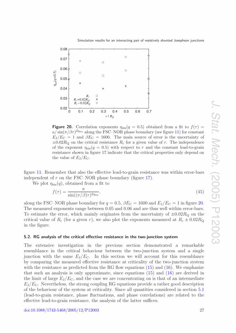
Figure 20. Correlation exponents ηsin(q = 0.5) obtained from a fit to f(τ) =a/ sin(π/βτ)2ηsin along the FSC–NOR phase boundary (see figure 11) for constantEJ/EC = 1 and βEC = 1600. The main source of error is the uncertainty of±0.02RQ on the critical resistance Rc for a given value of r. The independenceof the exponent ηsin(q = 0.5) with respect to r and the constant lead-to-grainresistance shown in figure 17 indicate that the critical properties only depend onthe value of EJ/EC.

figure 11. Remember that also the effective lead-to-grain resistance was within error-barsindependent of r on the FSC–NOR phase boundary (figure 17).

We plot ηsin(q), obtained from a fit to

f(τ) =a

sin((π/β)τ)2ηsin, (45)

along the FSC–NOR phase boundary for q = 0.5, βEC = 1600 and EJ/EC = 1 in figure 20.The measured exponents range between 0.05 and 0.06 and are thus well within error-bars.To estimate the error, which mainly originates from the uncertainty of ±0.02RQ on thecritical value of Rc (for a given r), we also plot the exponents measured at Rc ± 0.02RQ

in the figure.

5.2. RG analysis of the critical effective resistance in the two-junction system

The extensive investigation in the previous section demonstrated a remarkableresemblance in the critical behaviour between the two-junction system and a singlejunction with the same EJ/EC. In this section we will account for this resemblanceby comparing the measured effective resistance at criticality of the two-junction systemwith the resistance as predicted from the RG flow equations (15) and (16). We emphasizethat such an analysis is only approximate, since equations (15) and (16) are derived inthe limit of large EJ/EC, and the case we are concentrating on is that of an intermediateEJ/EC. Nevertheless, the strong coupling RG equations provide a rather good descriptionof the behaviour of the system at criticality. Since all quantities considered in section 5.1(lead-to-grain resistance, phase fluctuations, and phase correlations) are related to theeffective lead-to-grain resistance, the analysis of the latter suffices.

doi:10.1088/1742-5468/2005/12/P12003 27

http://dx.doi.org/10.1088/1742-5468/2005/12/P12003

J.Stat.M

ech.(2005)

P12003


R ζ R ζ

VDVD

I1I2B

R R

r

Ω

I

A C

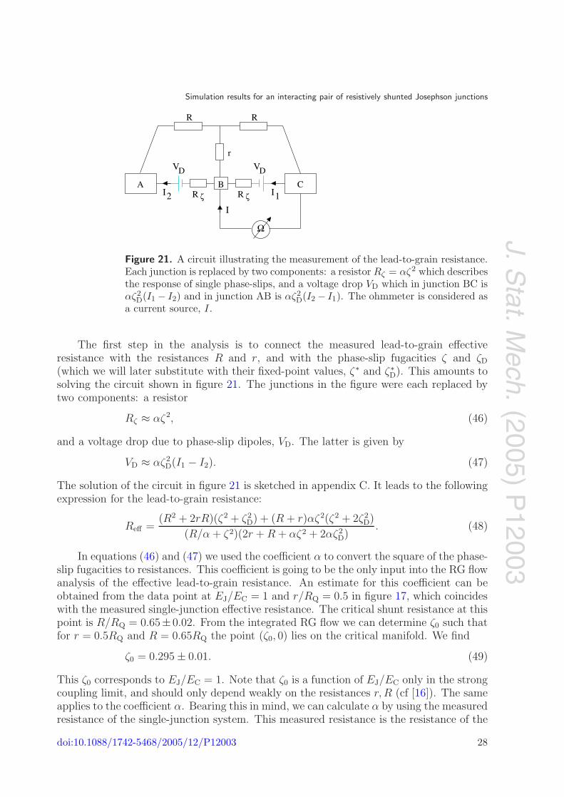
Figure 21. A circuit illustrating the measurement of the lead-to-grain resistance.Each junction is replaced by two components: a resistor Rζ = αζ2 which describesthe response of single phase-slips, and a voltage drop VD which in junction BC isαζ2

D(I1 − I2) and in junction AB is αζ2D(I2 − I1). The ohmmeter is considered as

a current source, I.

The first step in the analysis is to connect the measured lead-to-grain effectiveresistance with the resistances R and r, and with the phase-slip fugacities ζ and ζD

(which we will later substitute with their fixed-point values, ζ∗ and ζ∗D). This amounts to

solving the circuit shown in figure 21. The junctions in the figure were each replaced bytwo components: a resistor

Rζ ≈ αζ2, (46)

and a voltage drop due to phase-slip dipoles, VD. The latter is given by

VD ≈ αζ2D(I1 − I2). (47)

The solution of the circuit in figure 21 is sketched in appendix C. It leads to the followingexpression for the lead-to-grain resistance:

Reff =(R2 + 2rR)(ζ2 + ζ2

D) + (R + r)αζ2(ζ2 + 2ζ2D)

(R/α + ζ2)(2r + R + αζ2 + 2αζ2D)

. (48)

In equations (46) and (47) we used the coefficient α to convert the square of the phase-slip fugacities to resistances. This coefficient is going to be the only input into the RG flowanalysis of the effective lead-to-grain resistance. An estimate for this coefficient can beobtained from the data point at EJ/EC = 1 and r/RQ = 0.5 in figure 17, which coincideswith the measured single-junction effective resistance. The critical shunt resistance at thispoint is R/RQ = 0.65±0.02. From the integrated RG flow we can determine ζ0 such thatfor r = 0.5RQ and R = 0.65RQ the point (ζ0, 0) lies on the critical manifold. We find

ζ0 = 0.295 ± 0.01. (49)

This ζ0 corresponds to EJ/EC = 1. Note that ζ0 is a function of EJ/EC only in the strongcoupling limit, and should only depend weakly on the resistances r, R (cf [16]). The sameapplies to the coefficient α. Bearing this in mind, we can calculate α by using the measuredresistance of the single-junction system. This measured resistance is the resistance of the

doi:10.1088/1742-5468/2005/12/P12003 28

http://dx.doi.org/10.1088/1742-5468/2005/12/P12003

J.Stat.M

ech.(2005)

P12003


junction, αζ2, parallel to the shunt resistor, which equals RQ at criticality. Thus, forEJ/EC = 1 we have (figure 17)

αζ20 · RQ

RQ + αζ20

= 0.265 ± 0.015, (50)

from which we find

α = 4.15 ± 0.35. (51)

Now we have all the pieces to predict the effective lead-to-grain resistance, Reff , onthe FSC–NOR critical line EJ/EC = 1. By using equation (48) with the fixed-point valuesζ∗ and ζ∗

D from equation (27), and α from equation (51), we obtain the curve of Reff as afunction of r. The result of this calculation is shown in figure 17 by the dashed line. Onecan see that the resistance predicted by the RG changes little in the entire range, andremains in reasonably good agreement with the observed Monte Carlo Reff .

Note that we assumed that the measured resistance is due to the fixed-pointcharacteristics of the two-junction system. From section 4.2, however, we know that inthe vicinity of r = 0.75RQ, where the three phases meet, crossover effects are dominant.Therefore we expect the lead-to-grain resistance calculated in this section to deviate fromthe measured Reff in that vicinity. Another caveat for the current calculation is that it iscorrect up to second order in the phase-slip fugacities; fourth-order contributions to Reff

are neglected (although we keep fourth-order terms in equation (48)). These correctionsmay also account for deviations from the measured Reff .

6. The ICFP as a self-consistent fixed point

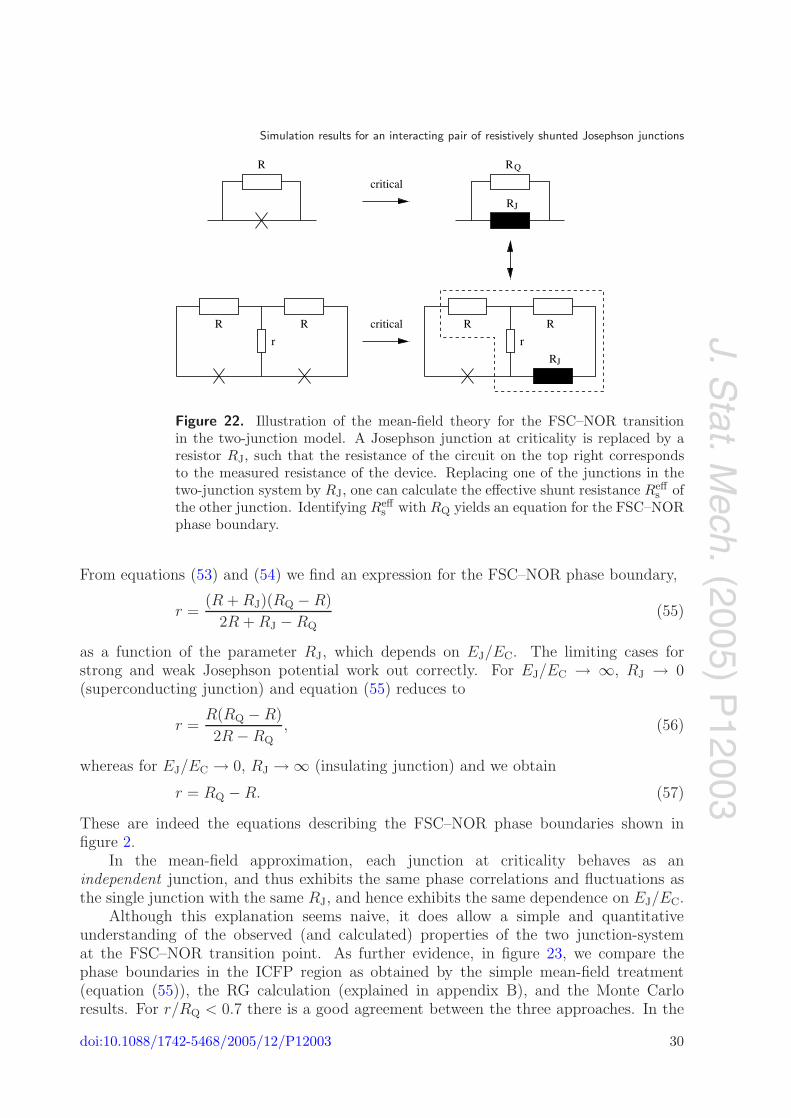
In the previous section we investigated the FSC–NOR transition extensively, anddemonstrated a remarkable resemblance between the two-junction and single-junctionsystems at criticality. We adequately explained this surprising resemblance using the RGfrom section 2. In this section, however, we provide yet another explanation, albeit ad hoc,for this resemblance. The alternative explanation is that the ICFP can be approximatedas a self-consistent fixed point. In such a mean-field theory, illustrated in figure 22, thephysics of a single junction emerges naturally. The idea behind this approach is that aJosephson junction undergoes an SC–NOR transition when its effective shunting resistanceis RQ.

Consider the two-junction system with phase-slip fugacities ζ0 (with ζD = 0) in bothjunctions. In mean field, one junction sees the other as an effective resistor (figures 22and 24) with resistance

RJ = αζ20 , (52)

where RJ is defined from equation (50). Therefore the effective shunting resistance oneach of the junctions is

Rs ≈ R +r (R + RJ)

r + R + RJ(53)

and criticality is obtained when

Rs = RQ. (54)

doi:10.1088/1742-5468/2005/12/P12003 29

http://dx.doi.org/10.1088/1742-5468/2005/12/P12003

J.Stat.M

ech.(2005)

P12003


J

R R

r

R R

r

R

R R

R

Q

critical

critical

J

Figure 22. Illustration of the mean-field theory for the FSC–NOR transitionin the two-junction model. A Josephson junction at criticality is replaced by aresistor RJ, such that the resistance of the circuit on the top right correspondsto the measured resistance of the device. Replacing one of the junctions in thetwo-junction system by RJ, one can calculate the effective shunt resistance Reff

s ofthe other junction. Identifying Reff

s with RQ yields an equation for the FSC–NORphase boundary.

From equations (53) and (54) we find an expression for the FSC–NOR phase boundary,

r =(R + RJ)(RQ − R)

2R + RJ − RQ(55)

as a function of the parameter RJ, which depends on EJ/EC. The limiting cases forstrong and weak Josephson potential work out correctly. For EJ/EC → ∞, RJ → 0(superconducting junction) and equation (55) reduces to

r =R(RQ − R)

2R − RQ

, (56)

whereas for EJ/EC → 0, RJ → ∞ (insulating junction) and we obtain

r = RQ − R. (57)

These are indeed the equations describing the FSC–NOR phase boundaries shown infigure 2.

In the mean-field approximation, each junction at criticality behaves as anindependent junction, and thus exhibits the same phase correlations and fluctuations asthe single junction with the same RJ, and hence exhibits the same dependence on EJ/EC.

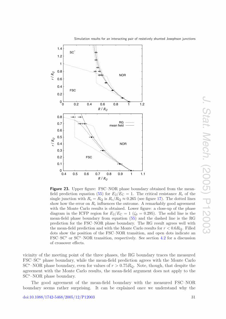
Although this explanation seems naive, it does allow a simple and quantitativeunderstanding of the observed (and calculated) properties of the two junction-systemat the FSC–NOR transition point. As further evidence, in figure 23, we compare thephase boundaries in the ICFP region as obtained by the simple mean-field treatment(equation (55)), the RG calculation (explained in appendix B), and the Monte Carloresults. For r/RQ < 0.7 there is a good agreement between the three approaches. In the

doi:10.1088/1742-5468/2005/12/P12003 30

http://dx.doi.org/10.1088/1742-5468/2005/12/P12003

J.Stat.M

ech.(2005)

P12003


0

0.1

0.2

0.3

0.4

0.5

0.6

0.7

0.8

0.4 0.5 0.6 0.7 0.8 0.9 1 1.1

r / R

Qr

/ RQ

R / RQ

R / RQ

FSC

NOR

RGmean field

0

0.2

0.4

0.6

0.8

1

1.2

1.4

0 0.2 0.4 0.6 0.8 1 1.2

SC*

FSC

NOR

Figure 23. Upper figure: FSC–NOR phase boundary obtained from the mean-field prediction equation (55) for EJ/EC = 1. The critical resistance Rc of thesingle junction with Rs = RQ is Rc/RQ ≈ 0.265 (see figure 17). The dotted linesshow how the error on Rc influences the outcome. A remarkably good agreementwith the Monte Carlo results is obtained. Lower figure: a close-up of the phasediagram in the ICFP region for EJ/EC = 1 (ζ0 = 0.295). The solid line is themean-field phase boundary from equation (55) and the dashed line is the RGprediction for the FSC–NOR phase boundary. The RG result agrees well withthe mean-field prediction and with the Monte Carlo results for r < 0.6RQ. Filleddots show the position of the FSC–NOR transition, and open dots indicate anFSC–SC∗ or SC∗–NOR transition, respectively. See section 4.2 for a discussionof crossover effects.

vicinity of the meeting point of the three phases, the RG boundary traces the measuredFSC–SC∗ phase boundary, while the mean-field prediction agrees with the Monte CarloSC∗–NOR phase boundary, even for values of r > 0.75RQ. Note, though, that despite theagreement with the Monte Carlo results, the mean-field argument does not apply to theSC∗–NOR phase boundary.

The good agreement of the mean-field boundary with the measured FSC–NORboundary seems rather surprising. It can be explained once we understand why the

doi:10.1088/1742-5468/2005/12/P12003 31

http://dx.doi.org/10.1088/1742-5468/2005/12/P12003

J.Stat.M

ech.(2005)

P12003


R R

r

R

A B C

D

Rζ +

Figure 24. Effective circuit in the mean-field approximation—taking phase-slipdipoles into account. Junction AB is approximated by a resistor with resistanceRζ = αζ2 which is due to single phase slips. In addition, phase-slip dipolesadd RD = αζ2

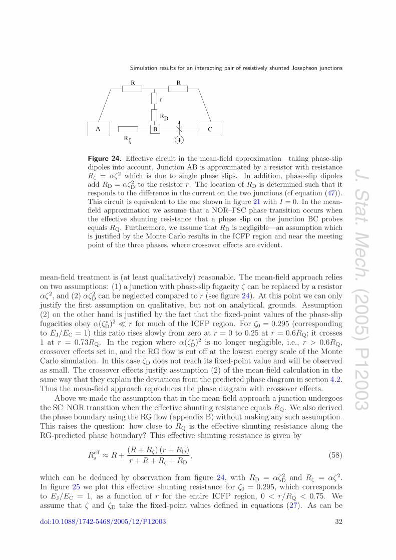
D to the resistor r. The location of RD is determined such that itresponds to the difference in the current on the two junctions (cf equation (47)).This circuit is equivalent to the one shown in figure 21 with I = 0. In the mean-field approximation we assume that a NOR–FSC phase transition occurs whenthe effective shunting resistance that a phase slip on the junction BC probesequals RQ. Furthermore, we assume that RD is negligible—an assumption whichis justified by the Monte Carlo results in the ICFP region and near the meetingpoint of the three phases, where crossover effects are evident.

mean-field treatment is (at least qualitatively) reasonable. The mean-field approach relieson two assumptions: (1) a junction with phase-slip fugacity ζ can be replaced by a resistorαζ2, and (2) αζ2

D can be neglected compared to r (see figure 24). At this point we can onlyjustify the first assumption on qualitative, but not on analytical, grounds. Assumption(2) on the other hand is justified by the fact that the fixed-point values of the phase-slipfugacities obey α(ζ∗

D)2 r for much of the ICFP region. For ζ0 = 0.295 (correspondingto EJ/EC = 1) this ratio rises slowly from zero at r = 0 to 0.25 at r = 0.6RQ; it crosses1 at r = 0.73RQ. In the region where α(ζ∗

D)2 is no longer negligible, i.e., r > 0.6RQ,crossover effects set in, and the RG flow is cut off at the lowest energy scale of the MonteCarlo simulation. In this case ζD does not reach its fixed-point value and will be observedas small. The crossover effects justify assumption (2) of the mean-field calculation in thesame way that they explain the deviations from the predicted phase diagram in section 4.2.Thus the mean-field approach reproduces the phase diagram with crossover effects.

Above we made the assumption that in the mean-field approach a junction undergoesthe SC–NOR transition when the effective shunting resistance equals RQ. We also derivedthe phase boundary using the RG flow (appendix B) without making any such assumption.This raises the question: how close to RQ is the effective shunting resistance along theRG-predicted phase boundary? This effective shunting resistance is given by

Reffs ≈ R +

(R + Rζ) (r + RD)

r + R + Rζ + RD, (58)

which can be deduced by observation from figure 24, with RD = αζ2D and Rζ = αζ2.

In figure 25 we plot this effective shunting resistance for ζ0 = 0.295, which correspondsto EJ/EC = 1, as a function of r for the entire ICFP region, 0 < r/RQ < 0.75. Weassume that ζ and ζD take the fixed-point values defined in equations (27). As can be

doi:10.1088/1742-5468/2005/12/P12003 32

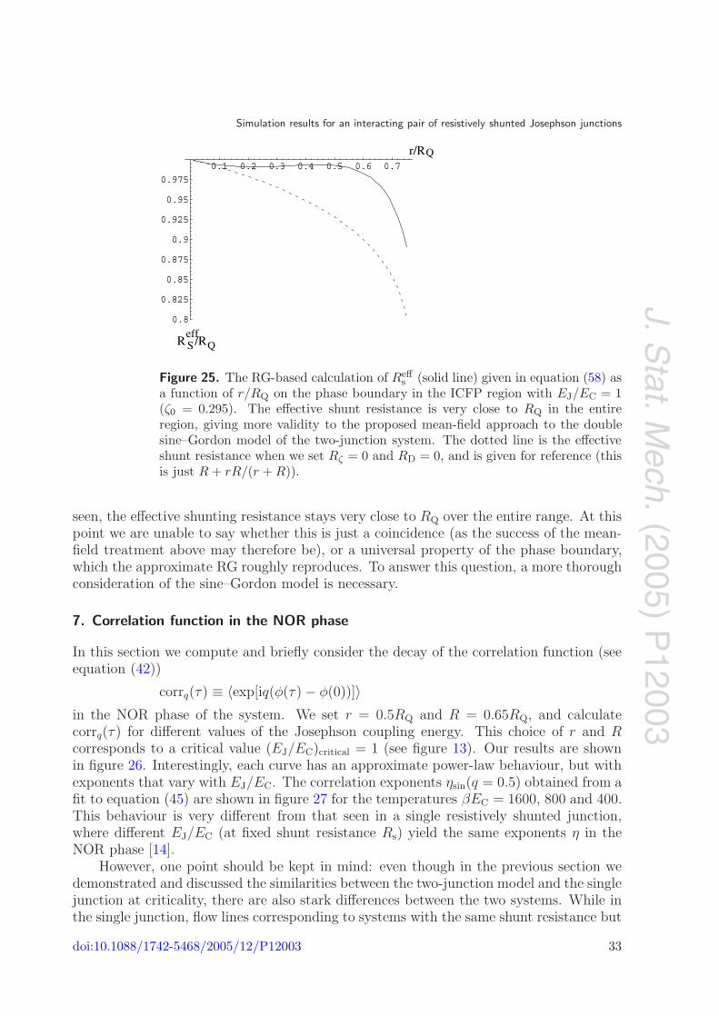
http://dx.doi.org/10.1088/1742-5468/2005/12/P12003

J.Stat.M

ech.(2005)

P12003


0.1 0.2 0.3 0.4 0.5 0.6 0.7

0.8

0.825

0.85

0.875

0.9

0.925

0.95

0.975

r/R Q

R /R effS Q

Figure 25. The RG-based calculation of Reffs (solid line) given in equation (58) as

a function of r/RQ on the phase boundary in the ICFP region with EJ/EC = 1(ζ0 = 0.295). The effective shunt resistance is very close to RQ in the entireregion, giving more validity to the proposed mean-field approach to the doublesine–Gordon model of the two-junction system. The dotted line is the effectiveshunt resistance when we set Rζ = 0 and RD = 0, and is given for reference (thisis just R + rR/(r + R)).

seen, the effective shunting resistance stays very close to RQ over the entire range. At thispoint we are unable to say whether this is just a coincidence (as the success of the mean-field treatment above may therefore be), or a universal property of the phase boundary,which the approximate RG roughly reproduces. To answer this question, a more thoroughconsideration of the sine–Gordon model is necessary.

7. Correlation function in the NOR phase

In this section we compute and briefly consider the decay of the correlation function (seeequation (42))

corrq(τ) ≡ 〈exp[iq(φ(τ) − φ(0))]〉in the NOR phase of the system. We set r = 0.5RQ and R = 0.65RQ, and calculatecorrq(τ) for different values of the Josephson coupling energy. This choice of r and Rcorresponds to a critical value (EJ/EC)critical = 1 (see figure 13). Our results are shownin figure 26. Interestingly, each curve has an approximate power-law behaviour, but withexponents that vary with EJ/EC. The correlation exponents ηsin(q = 0.5) obtained from afit to equation (45) are shown in figure 27 for the temperatures βEC = 1600, 800 and 400.This behaviour is very different from that seen in a single resistively shunted junction,where different EJ/EC (at fixed shunt resistance Rs) yield the same exponents η in theNOR phase [14].

However, one point should be kept in mind: even though in the previous section wedemonstrated and discussed the similarities between the two-junction model and the singlejunction at criticality, there are also stark differences between the two systems. While inthe single junction, flow lines corresponding to systems with the same shunt resistance but

doi:10.1088/1742-5468/2005/12/P12003 33

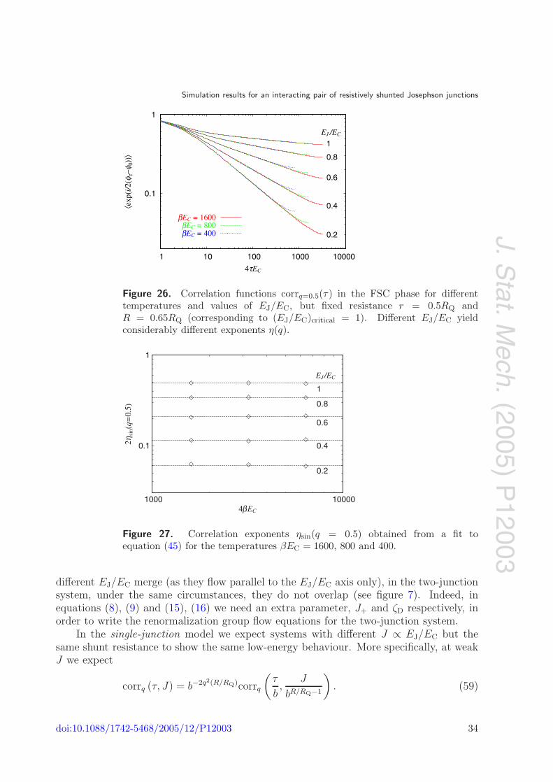
http://dx.doi.org/10.1088/1742-5468/2005/12/P12003

J.Stat.M

ech.(2005)

P12003


0.1

1

1 10 100 1000 10000

⟨exp

(i/2(

φ τ−φ

0))⟩

4τEC

EJ /EC

1

0.8

0.6

0.4

0.2

βEC = 1600βEC = 800βEC = 400

Figure 26. Correlation functions corrq=0.5(τ) in the FSC phase for differenttemperatures and values of EJ/EC, but fixed resistance r = 0.5RQ andR = 0.65RQ (corresponding to (EJ/EC)critical = 1). Different EJ/EC yieldconsiderably different exponents η(q).

0.1

1

1000 10000

2 ηsi

n(q=

0.5)

4βEC

EJ/EC

1

0.8

0.6

0.4

0.2

Figure 27. Correlation exponents ηsin(q = 0.5) obtained from a fit toequation (45) for the temperatures βEC = 1600, 800 and 400.

different EJ/EC merge (as they flow parallel to the EJ/EC axis only), in the two-junctionsystem, under the same circumstances, they do not overlap (see figure 7). Indeed, inequations (8), (9) and (15), (16) we need an extra parameter, J+ and ζD respectively, inorder to write the renormalization group flow equations for the two-junction system.

In the single-junction model we expect systems with different J ∝ EJ/EC but thesame shunt resistance to show the same low-energy behaviour. More specifically, at weakJ we expect

corrq (τ, J) = b−2q2(R/RQ)corrq

(τ

b,

J

bR/RQ−1

). (59)

doi:10.1088/1742-5468/2005/12/P12003 34

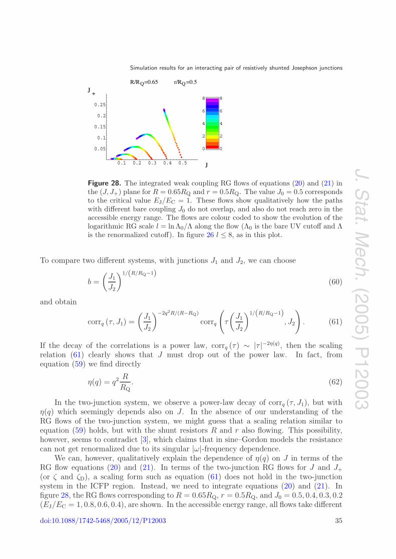
http://dx.doi.org/10.1088/1742-5468/2005/12/P12003

J.Stat.M

ech.(2005)

P12003


0.1 0.2 0.3 0.4 0.5

0.05

0.1

0.15

0.2

0.25

0

2

4

6

8

0

2

4

6

8

J

J +

R/R =0.65 r/R =0.5Q Q

Figure 28. The integrated weak coupling RG flows of equations (20) and (21) inthe (J, J+) plane for R = 0.65RQ and r = 0.5RQ. The value J0 = 0.5 correspondsto the critical value EJ/EC = 1. These flows show qualitatively how the pathswith different bare coupling J0 do not overlap, and also do not reach zero in theaccessible energy range. The flows are colour coded to show the evolution of thelogarithmic RG scale l = ln Λ0/Λ along the flow (Λ0 is the bare UV cutoff and Λis the renormalized cutoff). In figure 26 l ≤ 8, as in this plot.

To compare two different systems, with junctions J1 and J2, we can choose

b =

(J1

J2

)1/(R/RQ−1)(60)

and obtain

corrq (τ, J1) =

(J1

J2

)−2q2R/(R−RQ)

corrq

(τ

(J1

J2

)1/(R/RQ−1), J2

). (61)

If the decay of the correlations is a power law, corrq (τ) ∼ |τ |−2η(q), then the scalingrelation (61) clearly shows that J must drop out of the power law. In fact, fromequation (59) we find directly

η(q) = q2 R

RQ. (62)

In the two-junction system, we observe a power-law decay of corrq (τ, J1), but withη(q) which seemingly depends also on J . In the absence of our understanding of theRG flows of the two-junction system, we might guess that a scaling relation similar toequation (59) holds, but with the shunt resistors R and r also flowing. This possibility,however, seems to contradict [3], which claims that in sine–Gordon models the resistancecan not get renormalized due to its singular |ω|-frequency dependence.

We can, however, qualitatively explain the dependence of η(q) on J in terms of theRG flow equations (20) and (21). In terms of the two-junction RG flows for J and J+

(or ζ and ζD), a scaling form such as equation (61) does not hold in the two-junctionsystem in the ICFP region. Instead, we need to integrate equations (20) and (21). Infigure 28, the RG flows corresponding to R = 0.65RQ, r = 0.5RQ, and J0 = 0.5, 0.4, 0.3, 0.2(EJ/EC = 1, 0.8, 0.6, 0.4), are shown. In the accessible energy range, all flows take different

doi:10.1088/1742-5468/2005/12/P12003 35

http://dx.doi.org/10.1088/1742-5468/2005/12/P12003

J.Stat.M

ech.(2005)

P12003


paths in the (J, J+) space. Also, they are all far from saturating at J = J+ = 0. The latterobservation provides the reason for the slower decay of the correlations for higher J : inthe accessible energy range the two-junction system seems to have a larger effective J andJ+, the higher the bare J0 is. These finite J and J+, in turn, provide extra conductance inthe system, and thus strengthen phase coherence, and suppress the decay of correlations.

We furthermore note that the flow in the temperature range 400 < βEC < 1600(corresponding to 6 < l < 7.4) is rather slow, which might explain why there is hardlyany temperature dependence in the measured η (figure 27). However, we cannot rule outa scenario where the flows have actually converged to a set of distinct fixed points (withfor example different values of J+), although the origin of such additional fixed pointsremains unclear.

8. Conclusions

In this paper, we have presented an RG analysis and simulation results for a symmetrictwo-junction system. The phase diagram was found to contain all three phases predictedby theory: (i) fully superconducting (FSC), (ii) normal (NOR) and (iii) superconductingfrom lead to lead but normal from lead to grain (SC∗). Furthermore, the phase boundariesobtained by the Monte Carlo simulation agreed with the theoretical prediction, exceptfor deviations near the tricritical point where the three phases meet. These deviationswere interpreted as finite-temperature crossover effects, and give indirect evidence for theexistence of the intermediate coupling fixed point. The behaviour of correlation functionsin the NOR phase may also be indirect evidence for the flow of the coupling J+, aspredicted by the RG theory.

The two-junction system possesses the unusual ICFP region, in which the NOR–FSCtransition can be tuned by EJ/EC as well as by the dissipation strength. We calculatedthis phase boundary using the RG treatment of [1], and found that it fits the MonteCarlo result quite well (cf figure 12). Theoretically it was shown that in this region theproperties of the two-junction system are determined by a new intermediate coupling fixedpoint, with continuously varying exponents.

An efficient Monte Carlo algorithm was used to thoroughly investigate the intriguingICFP region and the NOR–FSC phase transition. We calculated the lead-to-grainresistance, average phase fluctuations, and phase correlations for several locations on thecritical NOR–FSC manifold. This manifold is two dimensional, and can be parameterizedby r and EJ/EC. For the various sets of (r, EJ/EC) on the NOR–FSC critical manifold wemade a surprising observation: the effective fixed-point lead-to-grain resistance, RAB, aswell as other critical properties of the two-junction model, were nearly identical to those ofa single junction (with the same EJ/EC) at criticality (Rs = RQ). Moreover, the effectivelead-to-grain resistance is within error-bars independent of r and R, and depends only onEJ/EC.

Given the success of the RG analysis of the two-junction model, we tried to useit in order to account for the above observations. Using simple scaling arguments, weextended the RG of [1] and section 2 to compute the effective lead-to-grain resistance atthe critical point. This calculation also yielded a nearly r-independent effective resistance,and since in the limit r = 0, R = RQ, the two-junction system and the single-junctionsystem coincide, the observations about the resemblance of the two systems seem to be

doi:10.1088/1742-5468/2005/12/P12003 36

http://dx.doi.org/10.1088/1742-5468/2005/12/P12003

J.Stat.M

ech.(2005)

P12003


satisfactorily explained. The approximate RG-based resistance calculation fitted the QMCresults quite well (figure 17).

But the observed similarity of the single- and two-junction systems could also bequalitatively interpreted in a more interesting way. The observation can be taken toindicate that, at criticality, each of the two junctions in the system sees an effectiveenvironment that imitates an Rs = RQ shunt, and therefore shows the same effectivefixed-point resistance and critical properties as a single isolated junction at criticality.This mean-field argument was developed in section 6, and it allowed us to predict thelocation of the FSC–NOR phase boundary at intermediate Josephson energy well withinerror bars (figure 23). In addition, we used the RG predictions to compute the effectiveshunt resistance for each junction, and we found an astonishing result: in most of theICFP region, the effective shunt for each junction does not deviate more than 1% fromRQ (figure 25).

The apparent success of a mean-field theory in this interacting system seems quiteremarkable. Even more so is the fact that the RG-based calculation of the effective shunton the critical manifold also yields with good accuracy RQ. This is indirect evidence foran internal structure in the coupled sine–Gordon theory that describes the two-junctionsystem. If this approximation turns out to be generally valid, it may also give insight intothe solution of coupled sine–Gordon models at intermediate couplings where no expansionscan be done and little is analytically known.

The relevance of our work goes well beyond the two junction system. A closelyrelated class of systems consists of resistively shunted Josephson junction arrays of two ormore dimensions (see e.g. [7]). The RG equations derived for the two-junction system [1]were shortly thereafter also derived for a two-dimensional triangular array of resistivelyshunted Josephson junctions in the weak coupling regime: in [13], Tewari et al showthat the weakly coupled triangular array undergoes a superconductor-to-metal transitionalmost identical to the direct NOR–FSC transition of the two-junction system (the RGequations for the two systems differ by one coefficient). Recall that this transition is inthe interesting and novel ICFP region. Tewari et al also considered the square lattice, inwhich the RG equation are third order in the Josephson coupling, a difference which isunimportant near the ICFP. Hence, the work presented in this paper also verifies manyof the results in [13].

In the future, we plan to adapt the Monte Carlo algorithm such that it can beapplied to sizable arrays of Josephson junctions. This would allow for the first time directcontrolled investigation of the Kosterlitz–Thouless NOR–SC∗ (normal–superconducting)transition in one-dimensional resistively shunted and free Josephson-junction arrays.Another interesting application for the algorithm would be Josephson-junction systemscoupled to quasi-particle dissipation [17].

Acknowledgments

We acknowledge support by the Swiss National Science Foundation and NSF grantPHY99-07949, as well as helpful discussions with S Chakravarty, E Demler and D Fisher.Part of this work was completed at the Kavli Institute for Theoretical Physics, UCSB. Weare also grateful for the hospitality of the Aspen Institute of Physics. The calculations

doi:10.1088/1742-5468/2005/12/P12003 37

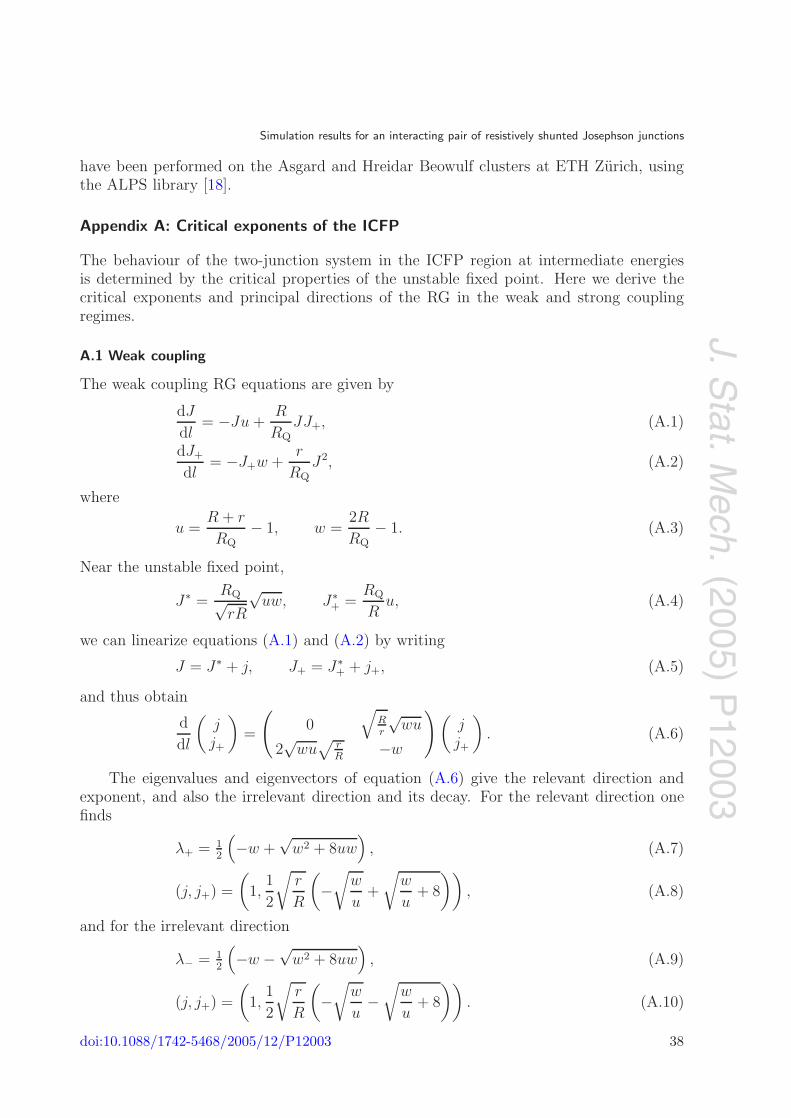
http://dx.doi.org/10.1088/1742-5468/2005/12/P12003

J.Stat.M

ech.(2005)

P12003


have been performed on the Asgard and Hreidar Beowulf clusters at ETH Zurich, usingthe ALPS library [18].

Appendix A: Critical exponents of the ICFP

The behaviour of the two-junction system in the ICFP region at intermediate energiesis determined by the critical properties of the unstable fixed point. Here we derive thecritical exponents and principal directions of the RG in the weak and strong couplingregimes.

A.1 Weak coupling

The weak coupling RG equations are given by

dJ

dl= −Ju +

R

RQ

JJ+, (A.1)

dJ+

dl= −J+w +

r

RQJ2, (A.2)

where

u =R + r

RQ− 1, w =

2R

RQ− 1. (A.3)

Near the unstable fixed point,

J∗ =RQ√rR

√uw, J∗

+ =RQ

Ru, (A.4)

we can linearize equations (A.1) and (A.2) by writing

J = J∗ + j, J+ = J∗+ + j+, (A.5)

and thus obtain

d

dl

(jj+

)=

(0

√Rr

√wu

2√

wu√

rR

−w

) (jj+

). (A.6)

The eigenvalues and eigenvectors of equation (A.6) give the relevant direction andexponent, and also the irrelevant direction and its decay. For the relevant direction onefinds

λ+ = 12

(−w +

√w2 + 8uw

), (A.7)

(j, j+) =

(1,

1

2

√r

R

(−

√w

u+

√w

u+ 8

)), (A.8)

and for the irrelevant direction

λ− = 12

(−w −

√w2 + 8uw

), (A.9)

(j, j+) =

(1,

1

2

√r

R

(−

√w

u−

√w

u+ 8

)). (A.10)

doi:10.1088/1742-5468/2005/12/P12003 38

http://dx.doi.org/10.1088/1742-5468/2005/12/P12003

J.Stat.M

ech.(2005)

P12003


Near the unstable fixed point we expect

j ∼ aT−λ+ + bT−λ−, j+ ∼ a+T−λ+ + b+T−λ−, (A.11)

where a and b are determined by the initial J (0) and J(0)+ . At very low T we are close to

the J = J+ = 0 fixed point and have

J ∼ T u, J+ ∼ T w. (A.12)

If the system is superconducting, which means that J (0) and J(0)+ are in the region in

which the couplings grow, then equation (A.11) still holds for intermediate temperatures,but as soon as the J are far from the ICFP, the system crosses over to the strong couplingregime, where

ζ ∼ T (RQ(R+r)/(2Rr+R2))−1, (A.13)

as follows from equation (17).

A.2 Strong coupling regime

The RG equations for the strong coupling case are

dζ

dl= −ζu +

RRQ

R2 + 2RrζζD, (A.14)

dζD

dl= −ζDv +

rRQ

R2 + 2Rrζ2, (A.15)

where

u =RQ(R + r)

2Rr + R2− 1, w =

2RRQ

R2 + 2Rr− 1. (A.16)

As in the weak coupling case we linearize these equations near the unstable fixed point

ζ∗ =R2 + 2rR

RQ

√rR

√uw, ζ∗

D =R2 + 2rR

RQRu, (A.17)

writing

ζ = ζ∗ + z, ζD = ζ∗D + zD, (A.18)

and thus obtain

d

dl

(zzD

)=

(0

√Rr

√wu

2√

wu√

rR

−w

) (zzD

). (A.19)

Equation (A.19) is essentially identical to equation (A.6), for the weak coupling case,except for the change of u, w to w, u. Therefore all other results can be copied from theprevious section as well. The eigenvalues and eigenvectors of the matrix in equation (A.19)are

λ+ = 12

(−w +

√w2 + 8uw

), (A.20)

(z, zD) =

(1,

1

2

√r

R

(−

√w

u+

√w

u+ 8

)), (A.21)

doi:10.1088/1742-5468/2005/12/P12003 39

http://dx.doi.org/10.1088/1742-5468/2005/12/P12003

J.Stat.M

ech.(2005)

P12003


and for the irrelevant direction

λ− = 12

(−w −

√w2 + 8uw

), (A.22)

(z, zD) =

(1,

1

2

√r

R

(−

√w

u−

√w

u+ 8

)). (A.23)

Near the unstable fixed point we expect

z ∼ aT−λ+ + bT−λ−, zD ∼ a+T−λ+ + b+T−λ−, (A.24)

just as for j and j+ in equation (A.11) for the weak coupling case.

Appendix B: Approximate calculation of the NOR–FSC phase boundary

By using the result of appendix A for the ICFP and the critical exponents and irrelevantdirections, equations (A.22) and (A.23), we can find an approximate implicit equationwhich can be solved for the critical R as a function of r and ζ0 (or J0). The calculationis identical for the two limits; we will demonstrate it for the strong coupling limit.

The calculation is based on the simple assumption that for r, R and ζ0 tuned to thecritical values, the critical RG flow line between the point (ζ = ζ0, ζD = 0) and the fixedpoint (ζ∗, ζ∗

D) given in equation (27) is a straight line. This is illustrated in figure B.1.The slope of the line representing the critical manifold is

tan θ = |zD/z| =1

2

√r

R

(√w

u+

√w

u+ 8

), (B.1)

where (z, zD) is defined in equation (A.23), and with u and w (which are functions of rand R) given in equation (A.16). The implicit equation for Rc is

ζD∗ = (ζ0 − ζ∗) tan θ. (B.2)

*

D

FSC

ζ

ζ

NOR

ζ0

θ

*D(ζ ,ζ )*

Figure B.1. We calculate the critical R as a function of r and ζ0 by assumingthat the flow from the initial state (ζ0, 0) to the fixed point (ζ∗, ζ∗D) is a straightline. This turns out to be a reliable approximation throughout the ICFP region.

doi:10.1088/1742-5468/2005/12/P12003 40

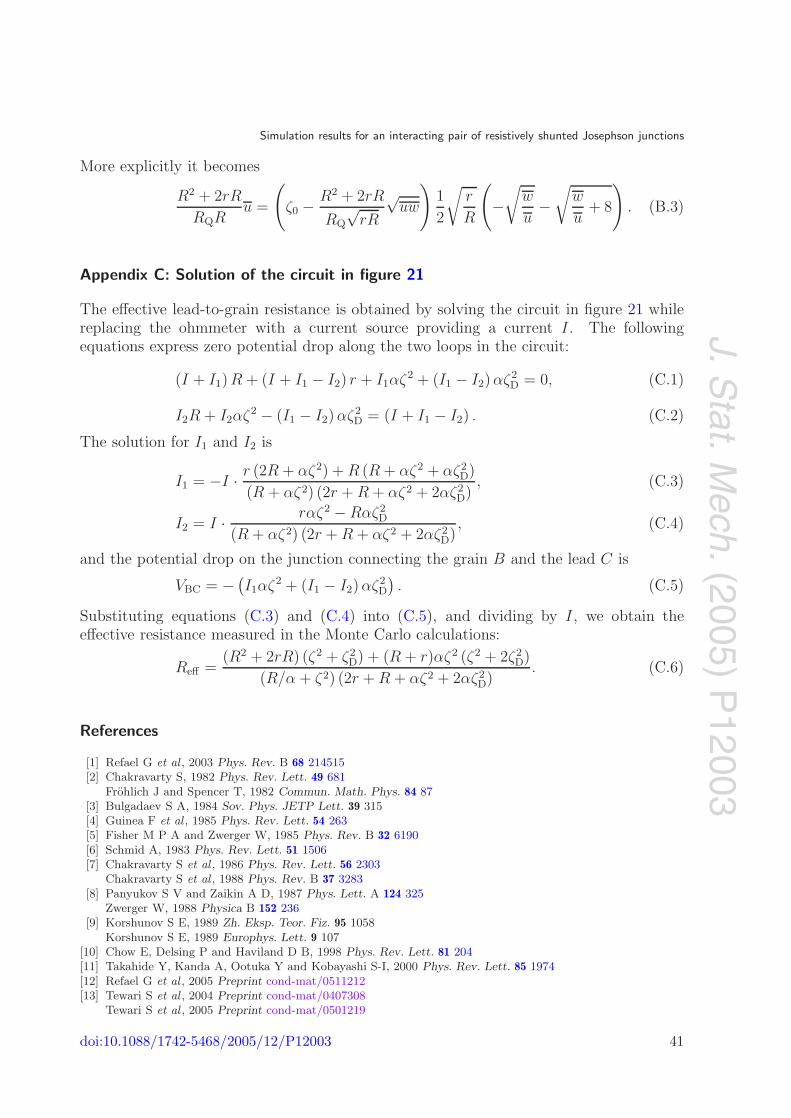
http://dx.doi.org/10.1088/1742-5468/2005/12/P12003

J.Stat.M

ech.(2005)P

12003


More explicitly it becomes

R2 + 2rR

RQRu =

(ζ0 −

R2 + 2rR

RQ

√rR

√uw

)1

2

√r

R

(−

√w

u−

√w

u+ 8

). (B.3)

Appendix C: Solution of the circuit in figure 21

The effective lead-to-grain resistance is obtained by solving the circuit in figure 21 whilereplacing the ohmmeter with a current source providing a current I. The followingequations express zero potential drop along the two loops in the circuit:

(I + I1)R + (I + I1 − I2) r + I1αζ2 + (I1 − I2)αζ2D = 0, (C.1)

I2R + I2αζ2 − (I1 − I2)αζ2D = (I + I1 − I2) . (C.2)

The solution for I1 and I2 is

I1 = −I · r (2R + αζ2) + R (R + αζ2 + αζ2D)

(R + αζ2) (2r + R + αζ2 + 2αζ2D)

, (C.3)

I2 = I · rαζ2 − Rαζ2D

(R + αζ2) (2r + R + αζ2 + 2αζ2D)

, (C.4)

and the potential drop on the junction connecting the grain B and the lead C is

VBC = −(I1αζ2 + (I1 − I2)αζ2

D

). (C.5)

Substituting equations (C.3) and (C.4) into (C.5), and dividing by I, we obtain theeffective resistance measured in the Monte Carlo calculations:

Reff =(R2 + 2rR) (ζ2 + ζ2

D) + (R + r)αζ2 (ζ2 + 2ζ2D)

(R/α + ζ2) (2r + R + αζ2 + 2αζ2D)

. (C.6)

References

[1] Refael G et al , 2003 Phys. Rev. B 68 214515[2] Chakravarty S, 1982 Phys. Rev. Lett. 49 681

Frohlich J and Spencer T, 1982 Commun. Math. Phys. 84 87[3] Bulgadaev S A, 1984 Sov. Phys. JETP Lett. 39 315[4] Guinea F et al , 1985 Phys. Rev. Lett. 54 263[5] Fisher M P A and Zwerger W, 1985 Phys. Rev. B 32 6190[6] Schmid A, 1983 Phys. Rev. Lett. 51 1506[7] Chakravarty S et al , 1986 Phys. Rev. Lett. 56 2303

Chakravarty S et al , 1988 Phys. Rev. B 37 3283[8] Panyukov S V and Zaikin A D, 1987 Phys. Lett. A 124 325

Zwerger W, 1988 Physica B 152 236[9] Korshunov S E, 1989 Zh. Eksp. Teor. Fiz. 95 1058

Korshunov S E, 1989 Europhys. Lett. 9 107[10] Chow E, Delsing P and Haviland D B, 1998 Phys. Rev. Lett. 81 204[11] Takahide Y, Kanda A, Ootuka Y and Kobayashi S-I, 2000 Phys. Rev. Lett. 85 1974[12] Refael G et al , 2005 Preprint cond-mat/0511212[13] Tewari S et al , 2004 Preprint cond-mat/0407308

Tewari S et al , 2005 Preprint cond-mat/0501219

doi:10.1088/1742-5468/2005/12/P12003 41

http://dx.doi.org/10.1103/PhysRevB.68.214515

http://dx.doi.org/10.1103/PhysRevLett.49.681

http://dx.doi.org/10.1007/BF01208373






http://dx.doi.org/10.1016/0375-9601(87)90020-X

http://dx.doi.org/10.1016/0921-4526(88)90095-6






http://dx.doi.org/10.1088/1742-5468/2005/12/P12003

J.Stat.M

ech.(2005)

P12003


[14] Werner P and Troyer M, 2005 Phys. Rev. Lett. 95 060201[15] Caldeira A O and Leggett A J, 1983 Ann. Phys., NY 149 374[16] Schon G and Zaikin A D, 1990 Phys. Rep. 198 237[17] Ambegaokar V, Eckern U and Schon G, 1982 Phys. Rev. Lett. 48 1745[18] Troyer M et al , 1998 Lecture Notes in Computer Science vol 1505 (Berlin: Springer) p 191

Alet F et al , 2005 J. Phys. Soc. Japan. Suppl. 74 30Source codes of the library are available from http://alps.comp-phys.org/

doi:10.1088/1742-5468/2005/12/P12003 42


http://dx.doi.org/10.1016/0003-4916(83)90202-6

http://dx.doi.org/10.1016/0370-1573(90)90156-V


http://alps.comp-phys.org/


























http://dx.doi.org/10.1088/1742-5468/2005/12/P12003

1 J. Stat .Mec h.for this simple system was shown to be remarkably com plex, with three distinct...

Documents

Transcript of 1 J. Stat .Mec h.for this simple system was shown to be remarkably com plex, with three distinct...