1

Inventory Management

Must-know Fundamentals

Operations ManagementDr. Mark P. Van Oyen

“Just the facts, Ma’am” Sgt. Friday“You’ve got to WIP it, WIP it good!” Devo

file: inven-lec.ppt

Types of Inventory

1. Raw materials and purchased parts. 3. Finished goods.

– Supplier– Distributor– Retailer

4. Replacement parts, tools, and supplies.

We are NOT talking about: Work in process (WIP).– Partially completed goods.– Goldratt warns about using “Economic Batch Quantity”

for shop floor lot-sizing… which is our EOQ as you’ll see.

Types of Inventory Demand

Independent demand items have demands which are not linked to the demand for other products. (Inventory focus)– Finished goods or end items (Saturns, laser pointers,

– These demands are typically forecasted.

We are NOT talking about Dependent demand items = Subassemblies or

component parts.– Derived from the demand of the independent demand items

(finished goods)

– Often dealt with using PUSH (MRP II, ERP) or PULL (Kanban, CONWIP, Bucket Brigades, etc.)

4

Independent

AA

d e

f1 f2 g1 g2

Dependent

Independent demand (Inventory). Dependent demand (MRP)

Independent Demand is usuallyfor end products (forecasted, uncertain)

X

B(2) C(1)

D(3) E(1) E(2) F(2)

Dependent Demand (MRP can back-figure release times givendue dates for independent demands)

Figure 14-6 of Stevenson

Functions of Inventory To meet anticipated demand. To protect against stockouts. (To meet unanticipated demand) To take advantage of quantity discounts, or to hedge against price

increases. To smooth production requirements.

– Level aggregate production plan is an example. To take advantage of order cycles.

– Efficiency in fixed costs of ordering or producing (e.g. share delivery truck)

To de-couple operations.– WIP inventory between successive manufacturing steps or

supply chain echelons (buffer stock) permits operations to continue during periods of breakdowns/strikes/storms.

Despite “Zero Inventory” zealots, an appropriate amount of inventory is a good thing in almost all systems!

6

Tradeoffs in the Size of Inventories

Inventories that are too high are expensive to carry, and they tie up capital.

Warehousing, transportation Greater risk of defects, even when carefully inventoried Market shifts leave seller with many unwanted parts

Inventories that are too low can result in reduced operational efficiency (machine starvation) poor service (delayed service, product substitution) lost sales (customer refuses raincheck, finds a more

reliable supplier)

7

Objectives/Controls of Inventory Control

Achieve satisfactory levels of customer service while keeping inventory costs under control.– Fill rate (probability of meeting a demand from inventory)– Inventory turnover ratio = Annual Sales / Average

Inventory Level = D / WIP– Others not focused one here: Average Backlog, Mean time

to fill order (Cycle Time) Profit maximization by achieving a balance in stocking,

avoiding both over-stocking and under-stocking. Controls:

– Decide how much to order/produce (Q)– Decide when to order/produce (ROP)

8

Profile of Inventory Level Over Time

Inventoryon hand

Q,Quantity

Receive order

Placeorder

Receive order

Placeorder

Receive order

Lead time

ReorderPoint,ROP

Average Usage rate

Time

Actual Usage

The Inventory Cycle

9

Costs

Holding costs or carrying costs (applied per unit of inventory)

– Associated with keeping inventory for a period of time.

– Capital tied up

– Warehousing and transportation

– Perishable products -OR- expected risk of damage to product

– Note that easiest calculation is (Holding cost rate/unit/yr) * (Average annual inventory level)

Ordering OR production costs (Fixed order set up + variable unit costs)

– For ordering and receiving inventory if ordering from a supplier, (Delivery charges, postage & handling, cost of purchasing dept. labor)

– OR production costs if we are the manufacturer . Shortage costs. (used in Newsvendor Model with demand uncertainty)

– Demand exceeds supply of inventory and a stockout occurs.

– Opportunity costs (lost sales and LOST CUSTOMERS!)

– Loss of good will, or, may need to substitute higher-cost item!

10

The Inventory Management Problem

Determine Inventory Policy:

How much to order or make? (Q)

When to order or make? (Reorder point)

How much to store in safety stock? To:

Minimize the cost of the inventory system

11

How Much to Order: Economic Order Quantity (EOQ) Models Objective:

Identify the optimal order quantity that minimizes the sum of certain annual costs that vary with order size.

Assumption: Fixed order quantity systems (don’t change order size dynamically over time)

We will consider here only the FIRST of 3 models:

– I. EOQ: all items delivered as a batch

– II. EOQ with gradual deliveries

– III. EOQ with quantity discounts (uses Model I assumptions)

12

Model I: (Basic) EOQ

“How Many Parts to Make at Once” by Ford Harris– Original 1913 version of this model.

Very simple - makes a lot of restrictive assumptions. It’s not realistic at first glance, but it is! Its usefulness keeps it alive!

Nicely illustrates basic tradeoffs that exist in any inventory management problem.

Basic Model Scenario: Own a warehouse from which parts (brake pads) are

demanded by customers. Periodically run out of parts and have to replenish inventory

by ordering from reliable suppliers.

13

EOQ Model I - Assumptions

Demand, D, is known and constant. Purchase Price, P, is known and constant. Fixed setup cost per order, S, independent of Q Holding cost C=H per unit per year. Lots of size Q are delivered in full (Production

Perspective: produce items and hold them in FGI until production is completed, at which time we ship them out).

There will be no stockouts, no backorders, no uncertainties!

Lead Time is known and constant.

14

Basic EOQ Model Assumptions

D = Demand rate is known and constant. (units/yr)[e.g. Sell brake pads with D = 60 pads/wk * 52]

P = Unit production/purchase cost - not counting setup or inventory costs ($/unit) [e.g. 2 $/pad]

S = Order set-up cost, constant per order ($/order) [e.g. 28.85 $/order]

C = H = Average annual carrying cost per unit ($/unit/yr.) [25% of purchase price/year = 0.50 $/yr]

Q = order quantity = decision variable [e.g. ?? Brake pads]

Inventory Cycle for Basic EOQ

Time

Inventory Level

Q = 600

Q/D = Length of Order Cycle

D = 60*52 pads/yr

10 wk.

16

Total Annual Cost Calculation

Order Frequency = F = D/Q = reciprocal of period e.g. (60 pads/wk)* 52 /600 pads = 52/10.

(orders/yr) Annual ordering cost is (# orders/year) * (order

setup cost) + (unit purch. cost) * (annual demand) = (D/Q)S + PD

Average inventory per order cycle: (Q+0)/2 = Q/2. why? use geometry to get average inv. Level (vs. calc.)

Annual carrying cost is (Q/2) C. Total annual Stocking Cost (TSC)

= [annual carrying cost + annual ordering cost]:

TSC = (D/Q)S + PD + (Q/2) C

17

Cost Minimization Goal

The Total-Cost Curve is U-Shaped

Ordering Costs

QO Order Quantity (Q)

An

nu

al C

os

t

(optimal order quantity)PD

18

Economic Order Quantity (EOQ)

There is a tradeoff between carrying costs and ordering costs!

EOQ is the value of Q that minimizes TSC. In this sense, the Q determined by the EOQ

formula is OPTIMAL given a simplistic model.

FYI only: EOQ is found by either:– Using calculus and solving (d/dQ)TSC = 0, the points of graph with

zero slope are either local maxima & minima, or,– Observing that the EOQ occurs where carrying and ordering costs are

equal, i.e., by solving (Q/2) C = (D/Q)S. [this is not a general method!]

19

EOQ Model I- Development

It turns out that Costs are minimized where ordering and carrying costs are equal.

Thus,

C

DSQ

QC

Q

DS

2

2

20

EOQ Model I- Example

Demand = 60 pads/wk

Ordering Cost, S = $28.85/order

Unit Carrying Cost = 25% of purchase price/yr.

Unit purchase price, P = $2.00/pad pads 600

)2($25.

)52)(60)(85.28(2

2

C

DSQ

21

The Concept of Reorder Point (ROP)

What inventory level should trigger/ control the placement of an order?

ROP = ReOrder Point = DDLT + SSDemand-During-Lead-Time + Safety-Stock

If Lead Time is 3 wks.,

ROP = (60)(3) = 180

22

Inventory Management Under Uncertainty

Demand or Lead Time or both uncertain Even “good” managers are likely to run out once in a

while (a firm must start by choosing a service level/fill rate)

When can you run out?– Only during the Lead Time if you monitor the

system. Solution: build a standard ROP system based on the

probability distribution on demand during the lead time (DDLT), which is a r.v. (collecting statistics on lead times is a good starting point!)

23

The Typical ROP System

ROP set as demand that accumulates during lead time

Lead Time

Average Demand

ROP = ReOrder Point

24

The Self-Correcting Effect- A Benign Demand Rate after ROP

ROP

Lead Time

Average Demand

Lead Time

Hypothetical Demand

25

What if Demand is “brisk” after hitting the ROP?

ROP >

Lead Time

Average Demand

Hypothetical Demand

SafetyStock

EDDLT

ROP = EDDLT + SS

When to Order The basic EOQ models address how much

to order: Q Now, we address when to order. Re-Order point (ROP) occurs when the

inventory level drops to a predetermined amount, which includes expected demand during lead time (EDDLT) and a safety stock (SS):

ROP = EDDLT + SS.

27

When to Order

SS is additional inventory carried to reduce the risk of a stockout during the lead time interval (think of it as slush fund that we dip into when demand after ROP (DDLT) is more brisk than average)

ROP depends on:– Demand rate (forecast based).– Length of the lead time.– Demand and lead time variability.– Degree of stockout risk acceptable to

management (fill rate, order cycle Service Level)

DDLT,EDDLT &Std. Dev.

28

The Order Cycle Service Level,(SL)

The percent of the demand during the lead time (% of DDLT) the firm wishes to satisfy. This is a probability.

This is not the same as the annual service level, since that averages over all time periods and will be a larger number than SL.

SL should not be 100% for most firms. (90%? 95%? 98%?)

SL rises with the Safety Stock to a point.

29

Safety Stock

LT Time

Expected demandduring lead time(EDDLT)

Maximum probable demand during lead time (in excess of EDDLT)defines SS

ROP

Qu

an

tity

Safety stock (SS)

30

Variability in DDLT and SS

Variability in demand during lead time (DDLT) means that stockouts can occur.– Variations in demand rates can result in a temporary

surge in demand, which can drain inventory more quickly than expected.

– Variations in delivery times can lengthen the time a given supply must cover.

We will emphasize Normal (continuous) distributions to model variable DDLT, but discrete distributions are common as well.

SS buffers against stockout during lead time.

31

Service Level and Stockout Risk

Target service level (SL) determines how much SS should be held.– Remember, holding stock costs money.

SL = probability that demand will not exceed supply during lead time (i.e. there is no stockout then).

Service level + stockout risk = 100%.

32

Computing SS from SL for Normal DDLT

Example 10.5 on p. 374 of Gaither & Frazier.

DDLT is normally distributed a mean of 693. and a standard deviation of 139.:– EDDLT = 693.– s.d. (std dev) of DDLT = = 139..– As computational aid, we need to relate this to

Z = standard Normal with mean=0, s.d. = 1» Z = (DDLT - EDDLT) /

33

Reorder Point (ROP)

ROP

Risk ofa stockout

Service level

Probability ofno stockout

Expecteddemand Safety

stock0 z

Quantity

z-scale

34

Area under standard Normal pdf from - to +z

z P(Z z)

0 .5

. 67 .75

.84 .80

1.28 .90

1.645 .95

2.0 .98

2.33 .99

3.5 .9998

StandardNormal(0,1)

0 z z-scale

P(Z <z)

Z = standard Normal with mean=0, s.d. = 1Z = (X - ) /

See G&F Appendix ASee Stevenson, second from last page

35

Computing SS from SL for Normal DDLT to provide SL = 95%.

ROP = EDDLT + SS = EDDLT + z ().

z is the number of standard deviations SS is set above EDDLT, which is the mean of DDLT.

z is read from Appendix B Table B2. Of Stevenson -OR- Appendix A (p. 768) of Gaither & Frazier:– Locate .95 (area to the left of ROP) inside the table (or as close as you

can get), and read off the z value from the margins: z = 1.64.

Example: ROP = 693 + 1.64(139) = 921SS = ROP - EDDLT = 921 - 693. = 1.64(139) = 228 If we double the s.d. to about 278, SS would double! Lead time variability reduction can same a lot of inventory

and $ (perhaps more than lead time itself!)

36

Single-Period Model: Newsvendor

Used to order perishables or other items with limited useful lives.– Fruits and vegetables, Seafood, Cut flowers.

– Blood (certain blood products in a blood bank)

– Newspapers, magazines, …

Unsold or unused goods are not typically carried over from one period to the next; rather they are salvaged or disposed of.

Model can be used to allocate time-perishable service capacity.

Two costs: shortage (short) and excess (long).

37

Single-Period Model

Shortage or stockout cost may be a charge for loss of customer goodwill, or the opportunity cost of lost sales (or customer!):

Cs = Revenue per unit - Cost per unit.

Excess (Long) cost applies to the items left over at end of the period, which need salvaging

Ce = Original cost per unit - Salvage value per unit.

(insert smoke, mirrors, and the magic of Leibnitz’s Rule here…)

38

The Single-Period Model: Newsvendor How do I know what service level is the best one, based

upon my costs? Answer: Assuming my goal is to maximize profit (at

least for the purposes of this analysis!) I should satisfy SL fraction of demand during the next period (DDLT)

If Cs is shortage cost/unit, and Ce is excess cost/unit, then

SLC

C Cs

s e

39

Single-Period Model for Normally Distributed Demand Computing the optimal stocking level differs slightly

depending on whether demand is continuous (e.g. normal) or discrete. We begin with continuous case.

Suppose demand for apple cider at a downtown street stand varies continuously according to a normal distribution with a mean of 200 liters per week and a standard deviation of 100 liters per week:

– Revenue per unit = $ 1 per liter

– Cost per unit = $ 0.40 per liter

– Salvage value = $ 0.20 per liter.

40

Single-Period Model for Normally Distributed Demand Cs = 60 cents per liter

Ce = 20 cents per liter.

SL = Cs/(Cs + Ce) = 60/(60 + 20) = 0.75

To maximize profit, we should stock enough product to satisfy 75% of the demand (on average!), while we intentionally plan NOT to serve 25% of the demand.

The folks in marketing could get worried! If this is a business where stockouts lose long-term customers, then we must increase Cs to reflect the actual cost of lost customer due to stockout.

41

Single-Period Model for Continuous Demand

Continuous example continued:– 75% of the area under the normal curve

must be to the left of the stocking level.– Appendix shows a z of 0.67 corresponds to a

“left area” of 0.749 – Optimal stocking level = mean + z (s.d.) =

200 + (0.67)(100) = 267. liters.

42

Tiny Tot Toys: A discrete example

Ave. Dem. = 6/day; D = 6 * 365 Demand distribution will be given (discrete) S = $10/order C = H= $2/unit/yr. Cs = $3.25/unit = penalty per unit stocked out Ce = ?? $/unit = average cost of having left-over

inventory at the end of period, based on C=H and variability in demand.

1. Use deterministic EOQ model to set Q

2. Use Newsvendor Model to set Safety Stock

43

Tiny Tot Toys - Optimizing Q

Ave. Dem. = D = 6*365 = 2190/yr S = $10/order C = H= $2/unit/yr.

1. Use deterministic EOQ model to set Q

days 25 / Length CycleOrder

1502

)10)(3656(22

DQC

DSQ

44

Use Newsvendor Model to set SL

2. We need to capture holding cost and inventory levels in Ce = avg. holding cost incurred over one order cycle (Why? Longer time frame. By the time we determine the excess, we have already ordered the next resupply. We’ll carry the excess for one cycle, at which point we decrease the reorder size to get things back on schedule.)

Ce = C*[Q/D]

= 2 $/yr/unit * [25 days / (365 days/yr)] = 0.1370 $/unit, Cs = 3.25 $/unit was given.

SL

325

325 13796%

.

. .

45

Wrap-up: SL for discrete distr.

Tiny Tot Toys desires SL = 96%. Demand is not Normally distributed; rather,

past data shows the following:

DDLT Probability CDF 25 .05 .05 35 .10 .15 45 .15 .30 55 .20 .50 65 .20 .70 75 .15 85 .10 95 .05 1.00

EDDLT = 60.0

46

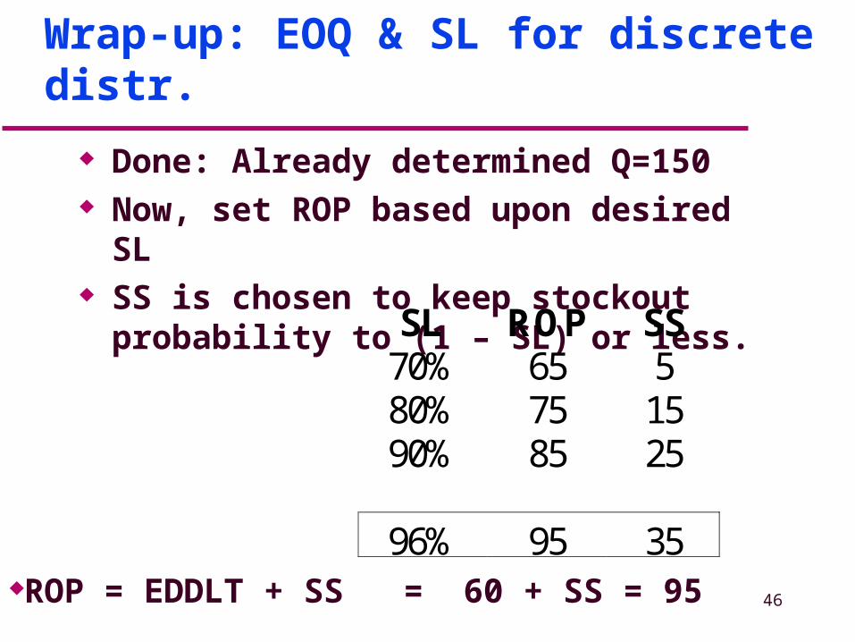
Wrap-up: EOQ & SL for discrete distr.

Done: Already determined Q=150 Now, set ROP based upon desired SL SS is chosen to keep stockout probability to (1 –

SL) or less. SL ROP SS 70% 65 5 80% 75 15 90% 85 25

96% 95 35

ROP = EDDLT + SS = 60 + SS = 95

47

Summary View

ROP >

Lead Time

Holding Cost = C[ Q/2 + SS] (approx.)(1)Order trigger by crossing ROP(2)Order a quantity up to (SS + Q)

SafetyStock

EDDLT

ROP = EDDLT + SS

Q+SS = Target Not full due to brisk

Demand after trigger