Kinetics of Food Biopolymer Film Dehydration: Experimental Studies and Mathematical Modelling

Rammile Ettelaie†*, Alison Tasker†, Jianshe Chen†, and Stefan Alevisopoulos‡

† Food Colloids Group, School of Food Science and Nutrition, University of Leeds, Leeds, LS2 9JT, UK.

‡ Henkel AG & Co. KGaA, Henkelstraße 67, 40589, Düsseldorf, Germany.

*Corresponding Author: Rammile Ettelaie

Food Colloid Group, School of Food Science and Nutrition, University of Leeds, Leeds LS2 9JT UK

E-mail : r.ettelaie@leeds.ac.uk, Telephone: +44 113 343 2981, Fax: +44 113 343 2982

1

ABSTRACT

The dehydration process in thin biopolymer based films, involving the two main

macromolecules in food systems, i.e. proteins and polysaccharides, has been investigated.

Experimental measurements of the weight loss of polymer films were carried out in an

enclosed Perspex chamber under controlled conditions of temperature, relative humidity and

air flow. We find that all the experimental moisture ratio data for films of pure biopolymers,

as well as their mixtures, can be superimposed on a single scaled dehydration curve.

Performing theoretical calculations, it has been shown that this curve cannot be described by

a moisture diffusion dominated drying process, irrespective of whether the film shrinkage is

included or ignored. We also derived an analytical expression for the evaporation controlled

drying. When the film shrinkage is fully accounted in the calculations, very good agreement

between the experiments and theoretically derived curve is obtained. However, the

theoretical results can be improved even further by considering a model that includes both

diffusion and evaporation processes, with diffusion being fast but nonetheless finite, so as to

only play a minor secondary role in dehydration of such films.

Theoretical models have also been extended to describe systems where the film shrinkage

can also arise from changes in the partial molar volumes, and not just loss of moisture. Using

a variable “effective” partial molar volume for water, the result provides a possible way of

modelling the entire drying process over different stages of dehydration, where the solid

phase adopts significantly contrasting structure.

2

1. INTRODUCTIONThin biopolymer films have many important applications in industry, particularly as

adhesives1, paints2, in the food industry as edible coatings3, and the pharmaceutical industry

as drug delivery systems.3, 4 The requirement and criteria are often very different for different

dehydration applications. It is therefore important to understand the mechanisms involved in

the drying process of these biopolymer films. For instance, if a film dries too rapidly, defects

such as cracks and bubbles can occur which weaken the films and reduce their performance.

On the other hand, if a film dries too slowly, dripping may occur for coating and labelling

applications. Temperature, relative humidity and air flow velocity are important external

parameters in controlling drying rate. However the diffusion of moisture within the internal

film structure is also a major factor in how the film dries. Drying, in some cases, can be split

into an initial constant rate period where free moisture from the surface is removed, followed

by two falling rate periods whereby diffusion is the main transfer mechanism. However, this

only applies to systems which start with a layer of saturated moisture on their surface and the

initial moisture loss can be compensated fully by the fast moisture diffusion. Water can be

present in different molecular environments depending on its interactions with the

surrounding molecules. Initially, most of the water in a polymer network is in free water

status (aw = 1) like those in a bulk phase water, surrounded by other water molecules, and can

diffuse through the system without significant restriction. This so-called free water is lost

during the constant rate and the first falling rate period. Once all the free water has

evaporated, the rate of dehydration slows and the second falling rate period becomes

apparent. Loosely bound water requires extra energy for either breaking up bonding or

internal evaporation. At this stage, diffusion of water could be either in liquid or in vapour or

in both. Practically, it is very difficult to differentiate the different mechanisms involved in

moisture diffusion. Therefore, an effective, moisture dependant diffusion coefficient is used

3

in the analysis of rate of dehydration. In most dehydration applications, bound water remains

untouched in the dried film. Often, and particularly in foods, an initial constant rate period is

not observed.5

During dehydration, changes in the structure of the polymer film may occur. The most

prevalent of these changes is film shrinkage, which is directly related to moisture loss due to

drying.6 As the film dries and moisture is lost, a pressure imbalance between the inside and

outside of the film develops. This pressure imbalance results in the build up of mechanical

stress within the film, which leads to possible shrinkage, collapse or cracking of the film in

order to release the stress. The increase of stress and its subsequent decrease due to structural

relaxation within a drying film has been experimentally measured by the authors.7 The

dynamics of stress evolution within the film depends significantly on the internal structure of

the film. The cracking of the film is most prevalent in drying of colloidal particulate

dispersions, or solutions of film forming polymers below their glass transition temperature,

where the structural relaxation times are long.8, 9 The porous structure allows moisture to

migrate to the surface through these channels without film shrinkage or loss of volume during

the drying process. Various models of transport, dealing in particular with the presence of

porous structures in foods and similarly related biological systems, have been reviewed by

Datta.10-12

Assumptions made in mathematical models to simulate such drying processes must reflect

these diverse behaviours in order to provide an accurate and reliable representation of the

drying process. During the drying of the biopolymer films used, initially, as moisture is lost

from within the film, the film shrinks due to the lack of a stress supporting structure. There

comes a point however, at which although moisture continues to be lost there is no further

shrinkage and the solid fraction forms a porous structure with a yield stress that can support

the stresses developed in the film. No further volume changes occur at this point. In order to

4

be able to model the entire dehydration process encompassing both these different

behaviours, it is important to consider the general case where effective molar volumes, if not

the true values, of both the solid and the water phases alter during the process. This will be

discussed in further detail in the theoretical considerations section.

There are many different methods reported to monitor and investigate aspects of drying.

NMR diffusion measurements have been used to investigate microstructure changes in

detergents during drying.13 This is a non-invasive technique which provided an insight into

the behaviour of individual droplets within detergents. Schmidt-Hansberg et al14 used

reflectometry to monitor the drying kinetics of polymer films. A laser beam was shone on the

sample and the reflected beam was detected using a silicon photodiode, throughout the drying

process, to collect data on the film thickness which was used to create moisture loss vs time

curves. The intensity of fluorescence given off by polymers as they dry has also been

monitored15, 16 where, as more water is released from a polymer, an increase in intensity of the

pyranine based fluorescence is seen. Results obtained using this method are supported by

gravimetric and volumetric data, and type II diffusion models, where Fick’s laws cannot

describe the entire process, fit the data well.

The simplest method for monitoring drying kinetics is the gravimetric method. This is a

macroscopic method that is the most prevalent of the techniques that are reported in the

literature.6, 17-19 It is easily applicable to all shapes and sizes for a wide range of materials. It is

a straightforward procedure where the sample is dried under controlled temperature and

relative humidity, and the sample is weighed over set time intervals. The method is popular

because the weight change with time is easy to measure, and if carried out in situ, does not

cause any disturbance to the sample’s drying environment which could potentially lead to

inaccuracies in the drying data. The method has also been used in the study of rehydration

5

and ingress of water into polymer coatings, although this is a somewhat different problem to

that of dehydration considered here.20

In most cases when thin films are dried, the controlling factor is diffusion of the moisture

within the film.21, 22 The rate of evaporation when moisture reaches the surface is assumed

rapid enough to be almost instantaneous and therefore does not influence the drying rate of

the film. This is reflected in the simplest mathematical models by taking the moisture content

at the surface of the film as always being at equilibrium with the moisture in the air above.

Furthermore, such models are mostly based on Fick’s second law of diffusion with either a

constant diffusion coefficient6, 17, 18, 23, 24, or in some a variable diffusion coefficient that

changes with moisture ratio. More sophisticated models attempt to take shrinkage of the

drying material into account, by using moving boundary conditions.19, 25 In most cases these

simple mathematical models have been found to give a reasonable fit to experimental data,

and in the literature many use these as a satisfactory approximation. However, as our work

demonstrates a more complex model may be required to give a more reliable representation

of the drying process.22

In this work the process of mass transfer during dehydration of several thin biopolymer films,

under controlled temperature and relative humidity conditions, is studied. Experimental

results will be compared with several mathematical models based on Fick’s second law of

diffusion and incorporating the following different scenarios: i) the dehydration involves both

constant and variable diffusion coefficients, as well as film shrinkage; ii) the diffusion is

instantaneous and the evaporation rate is the controlling factor; and iii) both diffusion and

evaporation have a role in controlling the drying rate. These models are discussed in detail in

the theoretical considerations section that follows. The ultimate aim of this work is to

establish a mathematical model which adequately describes the dehydration behaviour of thin

biopolymer films.

6

2. EXPERIMENTAL METHODThe samples investigated in the dehydration experiments were 18 wt% sodium caseinate

(purchased from Acros organics) solution, 7 wt% purity starch solution (provided by Henkel),

and a mixture of 9 wt% sodium caseinate and 4.5 wt% starch solution. The solutions were

prepared by dissolving the powder in distilled water at 90 °C under magnetic stirring for 1.5

h. Sodium azide (0.02 wt%) was added as a preservative, and 10 drops of an anti-foaming

agent were added to avoid the formation of bubbles.. All samples were stored at operating

temperature and used within three days of preparation.

The dehydration experiments were carried out in a purpose built, wood framed Perspex

chamber, with dimensions of 710 mm × 445 mm × 705 mm (length × width × height),

designed and made in house. The chamber has an accurate temperature control that allows the

chamber to be set at any temperature between room temperature and 50 °C. The relative

humidity was controlled reliably by continuous supply of dry air and wet air, bubbled through

pure water, into the chamber at a rate of 10L/min. The dry air was obtained by passing

controlled air through a drying column (Beko drypoint). The ratio of wet to dry air can be

controlled to achieve the desired relative humidity within the chamber. The chamber also has

a fan to create a gentle air flow so that air homogeneity can be maintained throughout the

entire system. The relative humidity conditions investigated include 20%, 30%, 40% and

50%, with the temperatures set to 30 °C, 40 °C and 50 °C. The chamber houses a beam

coating system which consists of a moveable platform with a stainless steel beam (80 mm x

12.6 mm x 0.4 mm) attached. On the left hand side wall of the chamber is a coating gate of

0.4 mm. A small volume of thermally equilibrated sample was first deposited on the beam.

The beam is then pulled though the coating gate at a constant speed using a stepper motor to

ensure an even coating of film, with a thickness of 0.4 mm and width of 10.6 mm, across the

full length of the beam. A diagram of the setup and the details of the procedure can also be

7

found in a previous study where the development of stress within drying films was studied.7

The coated beam is then placed on a balance inside the chamber and the weight loss is

monitored in situ at set time intervals for 4 hours.

3. THEORETICAL CONSIDERATIONS

In this section the drying process for a film, as applied to the biopolymer solutions discussed

above, is considered from a theoretical point of view. Within the body of the film, the process

of moisture transfer involves diffusion of water. On the upper surface of the film, i.e. the

surface exposed to the surrounding air, the loss of water is due to evaporation. It is assumed

that there is no loss of moisture through the substrate underneath the film and moisture loss

through the side surfaces is also negligible. We shall first highlight some of the issues and

complications that can arise in association with each of these two processes, before

presenting our mathematical analysis of the drying model. In the simplest case, one can

assume that the volume of the film remains constant throughout the drying process. This

occurs if the solid fraction in the polymer film has formed a porous layer through which the

water can migrate to the surface. Obviously, the yield stress of the porous structure formed in

such a case must be sufficient to withstand any capillary stresses induced during the loss of

moisture. Under such circumstances the much smaller diffusion of solid fraction can be

ignored. Furthermore, since the loss of water from any region in the film is not accompanied

by a change in the volume of that region, one may take the partial molar volume of the water

phase, on scales larger than the size of pores, as being effectively zero. When either the

internal diffusion or the surface evaporation is the dominant rate limiting process, simple

models of drying result. Analytical solutions for both of these models have been obtained

and extensively discussed in the literature.5, 22 Due to their inherent simplicity, and the

presence of closed form analytical solutions for each model, these have widely been used in

the fitting of the data from many drying experiments under a variety of circumstances.5 In

8

fact, their popularity has been such that they have been considered even in situations where

various assumptions inherent in the models, such as the requirement for a constant volume of

the sample, have not been strictly valid. In such cases often an empirical effective diffusion

coefficient, that is somewhat different to the real diffusion coefficient of water in the film, is

often used in order to partially compensate for the shrinkage and other complications not

present in the simple model.26

Where the changes in the volume of the film during drying are large, as would be the case if

there are no stress-supporting structures formed by the solid fraction, the approaches

discussed above can no longer be used. One immediate problem is that of specifying a

reference frame against which the diffusion fluxes are measured. As was originally pointed

out by Hartley and Crank27 there are many frames of reference that can be considered. For

example one may specify the diffusion fluxes relative to the substrate side of the sample or to

the film-air interface side. For a shrinking film these two frames result in different measured

fluxes. Other possibilities have been considered involving mean mass, mean molar or mean

volume reference frames.27, 28 So long as partial molar volumes of the components in the film

are not composition dependent, then diffusion coefficients measured in one reference frame

can easily be related to those obtained in another frame.29 Unless stated otherwise, in what

follows it is assumed that the diffusion process and all the related diffusion coefficients are

specified in the so called laboratory frame of reference, relative to the substrate.

There are two main factors that can contribute to changes in the volume of the sample.

Firstly, the more obvious one associated with the loss of the moisture. However, provided the

partial molar volumes of the components in the polymer solution are constant, independent of

the composition of the solution, the problem simplifies greatly. Here the reduction in the

volume remains strictly proportional to the amount of water that is lost at any stage

throughout the drying process. This makes it simpler to determine the location of the moving

9

air-film interface, knowledge of which is required for an analytical or indeed numerical

solution to the drying problem. The second factor influencing changes in the volume of the

film arises from the variation of the partial molar volumes of the two components with the

mix ratio. This frequently occurs in problems involving inter-diffusion of two metals or

metal oxides to form alloys.30 Variations arising as a result of changes in the partial molar

volumes add a substantial degree of complication to the analysis of the diffusion process.

Mathematical models of diffusion have been extended to account for these more complex

cases in relation to metal couples.31 Of course in such problems, unlike drying, the total mass

of the system remains a conserved quantity. This makes the use of constant mass reference

frame a more appropriate choice.28 In the drying problem, this type of variation in the volume

makes it that much more difficult to determine the location of the moving upper boundary.

However, since this knowledge is crucial in obtaining a solution to the equations describing

the drying process, the use of the constant mass reference frame is not as useful. A reference

frame with respect to the substrate is preferable in this case. Fortunately in many practical

situations involving the drying of food related biopolymer films, including systems studied

here, the partial molar volumes remain reasonably constant over a wide range of mixture

ratios. Nevertheless, since a theoretical analysis of changes arising from the variation of

partial molar volumes has not been fully considered in the context of the drying of the

biopolymer films, it is useful to first provide such a general treatment. The more familiar and

widely studied cases, involving constant partial molar volumes, emerge then as special limits

of this more general model. Before we present such an analysis, let us also first examine the

evaporation of water from the upper surface of the film.

The conditions prevalent at the air–film interface determine the rate at which water

evaporates from the film. These conditions include the nature of the solid phase, air

temperature and flow above the film and the amount of moisture in the film just beneath the

10

interface. For any given set of conditions there will be an equilibrium value of water content

(molar concentration), cweq, in the film that will be in equilibrium with the moisture in the air

above. Over a long period of time the water concentration in the film will approach cweq

everywhere in the dried film. In general the rate of water loss per unit surface area of the film

will be a function of (cw(L,t) cweq), where cw(L,t) is the concentration of water on the surface

at time t and L is the thickness of the film. The function can be expanded in powers of

(cw(L,t) cweq ) and provided the difference between c(L) and cw

eq is small, only the linear

term needs to be retained.

f (cw (L, t )−cweq)≈−K (cw (L ,t )−cw

eq ) . (1)

The approximation remains a rather good one, even for relatively large values of

(cw(L,t) cweq ). The value of K captures all the temperature dependence and other factors

related to the evaporation of the water from the film on the surface, but otherwise is a

constant for a given set of conditions. It is known as the drying constant.22

3.1. Drying Limited by Evaporation. If the diffusion of moisture is a relatively fast

process in the film, then the only important factor in limiting the drying is the evaporation.

This occurs for sufficiently small K, large water diffusion coefficient, D, and in thin films

where D/(KL) >> 1. Under such circumstances the water concentration gradients are small

across the film thickness. One may take the concentration of water as being uniform

throughout the film cw(z,t) = cw(L,t) = cw(t), where z is the distance into the film as measured

from the substrate. For cases with no shrinkage this leads to a very simple model that can

readily be solved to give an exponential decrease in the concentration of water with time,32

cw(t) = cweq + (cw(0) cw

eq )exp(-Kt/L) . Therefore let us consider the more interesting case

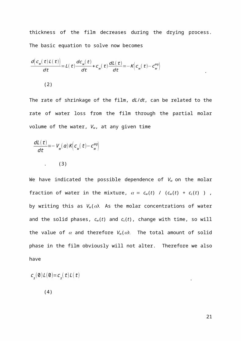
where the thickness of the film decreases during the drying process. The basic equation to

solve now becomes

11

d (cw ( t )L( t ))dt

=L( t )dcw( t )

dt+cw ( t )

dL( t )dt

=−K (cw( t )−cweq)

. (2)

The rate of shrinkage of the film, dL/dt, can be related to the rate of water loss from the film

through the partial molar volume of the water, Vw, at any given time

dL( t )dt

=−V w (α )K (cw ( t )−cweq )

. (3)

We have indicated the possible dependence of Vw on the molar fraction of water in the

mixture, cw(t) / (cw(t) + cs(t) ) , by writing this as Vw(As the molar concentrations of

water and the solid phases, cw(t) and cs(t), change with time, so will the value of and

therefore Vw( The total amount of solid phase in the film obviously will not alter.

Therefore we also have

cs (0 )L(0 )=c s( t )L (t ) . (4)

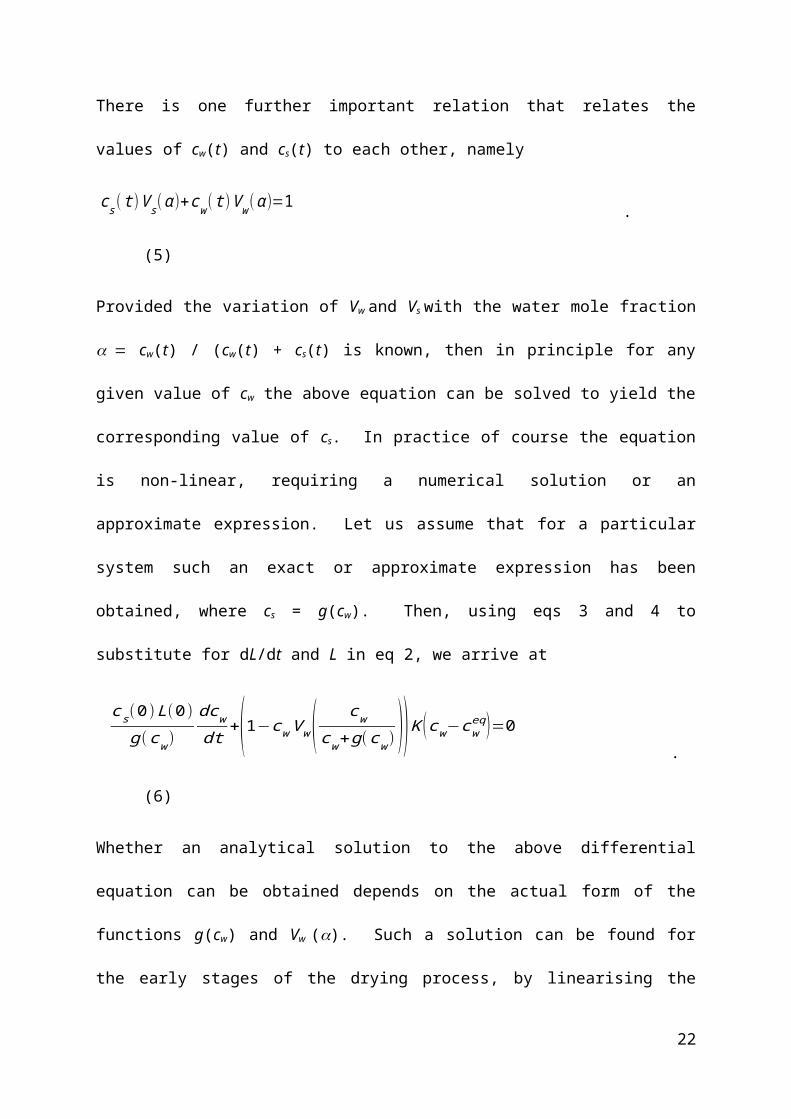
There is one further important relation that relates the values of cw(t) and cs(t) to each other,

namely

cs ( t )V s( α )+cw( t )V w (α )=1 . (5)

Provided the variation of Vw and Vs with the water mole fraction cw(t) / (cw(t) + cs(t) is

known, then in principle for any given value of cw the above equation can be solved to yield

the corresponding value of cs. In practice of course the equation is non-linear, requiring a

numerical solution or an approximate expression. Let us assume that for a particular system

such an exact or approximate expression has been obtained, where cs = g(cw). Then, using

eqs 3 and 4 to substitute for dL/dt and L in eq 2, we arrive at

cs( 0)L(0)g(cw )

dcw

dt+(1−cw V w ( cw

cw+g(cw )))K (cw−c weq )=0

. (6)

12

Whether an analytical solution to the above differential equation can be obtained depends on

the actual form of the functions g(cw) and Vw (). Such a solution can be found for the early

stages of the drying process, by linearising the functions around the initial value of cw.

Another special but important case, involves systems for which Vw and Vs are constant. As

mentioned before, many biopolymer solutions behave in this way, at least down to the very

last stages of drying. For these systems it is easier to work with the volume fraction of water

= cwVw. The volume fraction of the solid phase is then 1 = csVs. With partial molar

volumes independent of the composition, function g(cw) = (1 cwVw) / Vs = (1 ) / Vs.

Multiplying both sides of eq 6 by Vw we find

dφdt

= −K(1−φ (0)) L(0 )

(1−φ )2 (φ−φeq)

, (7)

where (0) is the initial volume fraction of the water in the film and eqis its equilibrium

value. The above differential equation can be solved to give an explicit relation between time

t and volume fraction of water in the system as follows:

1(1−φ)

− 1(1−φ (0))

+ 1(1−φeq )

ln [ (1−φ(0 ))(φ−φeq)

(1−φ )(φ(0 )−φeq) ] = −K (1−φeq )L(0 )(1−φ(0 ))

t

(8)

The results predicted by eq 8 is substantially different to that of the simple model not

accounting for the film shrinkage, when eq and (0) are not so small. However, for small

values of these quantities i.e. eq << 1 and (0) << 1, the equation predicts the same

exponential behaviour

13

(eq) / (0) - eq) = exp(-Kt/L(0) as the one obtained by the simple model. This is because

at small values of eq and (0), the term cw(dL/dt) becomes much smaller that L(dcw/dt) in eq

2, and hence the shrinkage of the film can be safely neglected. In the next section results

obtained from eq (8) will be compared with our experimental data involving drying of casein

and starch solution based films.

3.2. General Model for the Drying Film. In this section we will discuss the drying process

in which diffusion, evaporation and shrinkage of the film are all significant and none may be

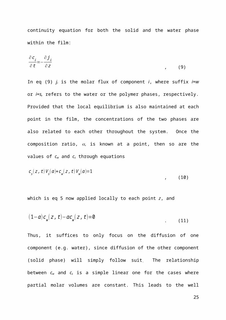
ignored. The diffusion process has to satisfy a number of basic relations, the most obvious of

which is the continuity equation for both the solid and the water phase within the film:

∂ci

∂ t=−

∂ ji

∂ z , (9)

In eq (9) ji is the molar flux of component i, where suffix i=w or i=s, refers to the water or the

polymer phases, respectively. Provided that the local equilibrium is also maintained at each

point in the film, the concentrations of the two phases are also related to each other

throughout the system. Once the composition ratio, is known at a point, then so are the

values of cw and cs through equations

cs ( z , t )V s (α )+cw ( z , t )V w( α )=1, (10)

which is eq 5 now applied locally to each point z, and

(1−α )cw ( z ,t )−αcw ( z ,t )=0 . (11)

Thus, it suffices to only focus on the diffusion of one component (e.g. water), since diffusion

of the other component (solid phase) will simply follow suit . The relationship between cw and

cs is a simple linear one for the cases where partial molar volumes are constant. This leads to

14

the well known situation for which the diffusion coefficient of both components are identical,

often referred to as the inter-diffusion coefficient.28, 29 To relate the diffusion of the two

components in these more general cases, let us differentiate both sides of eq 10 with respect

to z. We have

V w

∂ cw

∂ z+V s

∂ cs

∂ z=0

. (12)

The above equation is obvious when Vw and Vs are composition independent, but it also holds

more generally. This can be seen from the fact that

cw

∂V w

∂ z+cw

∂V w

∂ z=(cw+cs )(α

dV w

dα+(1−α )

dV s

dα )∂ α∂ z

=0. (13)

That the term in the bracket in the above equation is zero follows from the generalised form

of Denham-Gibbs equation, valid for all partial molar quantities.33 It can easily be derived by

considering changes in the volume of a uniform mixture of nw moles of water and ns moles of

polymer solid phase and the fact that the volume, V, is a function of state. In other words

2V/(nwns) = (Vs/nw)=(Vw/ns).

A very similar argument can be applied to the derivative of eq (10) with respect to time to

obtain

V w

∂ cw

∂ t+V s

∂ cs

∂ t=0

, (14)

which in combination with the continuity equations, eq (9), may also be written as

V w

∂ jw

∂ z+V s

∂ j s

∂ z=0

. (15)

Equations 9 to 15 apply quite generally to any two phase system, so long as the local

equilibrium is maintained at each point throughout the system. They are valid irrespective of

15

the laws that govern the dependence of the diffusion fluxes on concentrations. However, at

this stage a choice has to be made with regards to the relations governing the dependence of

diffusion fluxes on gradients of thermodynamic quantities. Several such laws have been

suggested over a number of years of which Fick’s first law, Maxwell-Stefan’s law or

Onsager’s flux law are amongst the best known and most widely used.28 In the present

discussion it is assumed that the flux relation for the water phase, though not necessary the

solid phase, can be described by Fick’s law

jw=−Dw (α )∂ cw

∂ z . (16)

The symbol Dw() in the above equation denotes the compositional dependent diffusion

coefficient of water, as measured in our chosen laboratory reference frame. It must be

stressed that this is a phenomenological relation the validity of which has to be verified

experimentally for the particular system of interest. Indeed, there are many situations, and in

particular with regards to diffusion of water in glassy polymer films, where Fick’s law is not

always obeyed.34-36 In other situations an equation similar to eq 16 can be developed only by

redefining the length scale in a position dependent manner, and by expressing the

concentrations in units consistent with this variable.27, 37 Substituting eq 16 into eq 9 for the

water phase, leads to the familiar Fick’s second law

∂cw

∂ t= ∂

∂ z (Dw (α )∂ cw

∂ z ) . (17)

As the concentration of moisture evolves with time across the film thickness, the

concentration of the solid phase, cs, has to follow suit in a manner dictated by eq 10 and 14.

Since the aim is to eliminate all references to cs in the equations governing the drying

process, we will consider the temporal variation of at each point, instead of cs. This is also

useful as, more often than not, the experimental data for partial molar volumes are given as

16

functions of the mole fraction of the constituent components. To obtain the required

equation, we express cw in terms of using eq 10 and 11; cw = Vs + Vw ].

Differentiating both sides of this equation with respect to time and rearranging we obtain

∂α∂ t

=[ ((1−α )V s+αV w )2

V s ] ∂ cw

∂ t=[ ((1−α )V s+αV w)2

V s ][ ∂∂ z (D(α )

∂ cw

∂ z )] .(18)

Equation 18 is particularly convenient for use in a finite difference or other similar numerical

schemes26, 38, since (cw/t) is determined at each time step using eq 17. By updating the

value of throughout the system the values of Vw and Vs can be refreshed at each point too.

Equations 17 and 18 have to be solved by imposing the appropriate boundary conditions to

the film. At the bottom surface, in contact with the substrate, these are jw(0,t)= js(0,t)= 0,

leading to

∂cw

∂ t=

∂cs

∂ t=0

. (19)

At the upper surface, where the evaporation of water takes place, one has

cwdLdt

− jw=−K (c w(L , t )−cweq )

. (20a)

for the water phase. The corresponding equation for the solid phase reads as follows:

csdLdt

− js=0. (20b)

The rate of change of the film thickness is denoted by dL/dt. These conditions follow directly

from eq 1 for the evaporation and the continuity equations for each phase at the air–film

interface.

17

Multiplying eq (20a) by Vw and eq (20b) by Vs and adding the two together one obtains the

rate of shrinkage of the film given by

dLdt

=V w jw+V s js−V w K ( cw(L , t )−cweq )

. (21)

The flux (Vw jw + Vs js ) in eq (21) above, when not equal to zero, indicates the presence of the

so called Darken velocity39, 40 and the related Kirkendall effect41, 42 rather well known in the

field of metallurgy. This effect manifests itself as a movement of marker non-diffusing

entities relative to the substrate. From a theoretical view, the effect has been analysed in

great detail in many different studies and has been the subject of several excellent reviews in

the literature.37, 43 It suffices here to mention that for a system where the local equilibrium

conditions are achieved quickly, and thus eq 10 prevails throughout the film, it can only

occur if the partial molar volumes change with the mixture ratio. Conversely, the presence of

the effect in a two component system where partial molar volumes are constant indicates that

the two constituent components are not in local equilibrium with each other, at least in some

regions in the system.

The reference to the solid phase can once again be removed from the above equation by

expressing js in terms of jw. To do so we integrate eq 15 from 0 to a given height z into the

film to obtain

j s( z ,t )=−∫0

z V w

V s

∂ jw

∂ z ' d z '=

−V w

V sjw+∫

0

z

jw∂(V w /V s )∂α

∂α∂ z ' d z '

. (22)

With eq 22 substituted in 21, we finally obtain the required equation describing the shrinkage

of the film purely in terms of the concentration and diffusion fluxes for the water phase:

18

dLdt

=V s∫0

z

jw (z ' ,t ))∂(V w /V s )

∂ α∂ α∂ z ' d z ' −V w K ( cw(L , t )−cw

eq ). (23)

Equations 16-18, together with the boundary conditions 19 and 20 and eq 23 for the rate of

shrinkage of the biopolymer film completely describe the diffusion–evaporation process.

Furthermore, they do so in a way that is fully consistent with the presence of local

equilibrium, as imposed by eq 10 at each point. Using these equations, a numerical scheme

can easily be implemented now to simulate the drying process. In such a scheme, it will be

even more convenient if the integral term in the above equation could be reduced to a form

which only involves local quantities at the air–film interface. We have not been able to

obtain such an expression for the integral. The presence of this integral term in eq 23 reflects

the fact that the shrinkage of the film depends on the changes in the mix ratio and thus those

in the values of the partial molar volumes, occurring not only on the surface but throughout

the whole of the film, all the way down to the substrate. Of course, when the partial molar

volumes are constants, then no such considerations will arise and this non-local term should

disappear. This is clearly the case in eq 23. We shall discuss the special case involving

constant partial molar volumes next and show how the equations derived above take on their

more familiar forms in such a circumstance.

3.3. Systems Involving Constant Partial Molar Volumes. When the partial molar volumes

of the constituent components are not dependent on the composition ratio, the equations

describing the drying process simplify significantly. In many biopolymers solutions this

condition is satisfied quite well over a large range of composition mix ratios. It is only at the

very last stages of the drying, where major changes in the structure of the film may occur,

that the assumption begins to be violated. As we had done in the analysis of the case

involving the drying process limited by evaporation, once again it is easier to work with the

19

volume fraction of water, = Vwcw. Thus, multiplying both sides of eq 17 by Vw the

moisture diffusion equation becomes

∂φ∂ t

= ∂∂ z (Dw( φ) ∂φ

∂ z ) . (24)

We now assume that the variation of the compositional dependent diffusion coefficient is

provided in terms of rather than . It is also immediately apparent that the diffusion

equation for the evolution of the volume fraction of the solid phase (1) is identical to eq

24, implying the expected result, Dw() = Ds(). So long as the diffusion coefficients are

given as a function of , eq 18 is redundant and need not be considered further. The fact that

the partial molar volumes are constant implies that the volume is now a conserved quantity in

the problem. That is to say that the volume of the remaining film and that of the evaporated

water together always equal the initial volume of the film. This requires

dLdt

=−K (φ−φeq)

. (25)

The above equation also results directly from eq 23 when Vw and Vs are constant, whereupon

the integral term in the equation vanishes. Finally, the boundary condition 19 at the substrate

side remains the same, while eq 20a at the air–film interface, z = L, can now be written as

D(φ ) ∂φ∂ z

=−K (1−φ )(φ−φeq ) . (26)

The presence of a moving boundary condition in the problem is not desirable. It can be

difficult to implement in a simple finite difference type numerical scheme and may require

redefinition of the grid as the film shrinks relative to the grid size. This can be a source of

20

numerical errors in the solution. One possible way to avoid such a problem would be to use a

set of coordinate system, y, where the length scale is continuously redefined by the thickness

of the film at time t:

y= zL( t ) . (27)

In the new coordinate systems the air–water interface is always at y = 1. We also define

θ=L( t )φ , (28)

such that

∫0

L( t )

φ dz=∫0

1

θ dy. (29)

In terms of our new length scale, the diffusion coefficient becomes D* = Dw/(L(t))2, while the

diffusion equation, eq 24, now turns into a diffusion-convection equation (see appendix A):

∂θ∂ t

= ∂∂ y (D¿ ∂θ

∂ y+ y

LdLdt

θ). (30)

Numerically it is much more convenient to implement a solution to eq 30, which now has to

be solved with a fixed boundary condition

D¿ ∂θ∂ y

=−K (1−θL )( θ

L−φeq)

, (31)

at y = 1, rather than the moving boundary condition for eq 24. We have implemented a

simple finite difference scheme to solve eq 30 in conjunction with eq 25. The solutions thus

21

obtained will once again be compared to our experimental results once they are discussed in

the next section.

4. RESULTS

4.1. The kinetics of Biopolymer Dehydration. The three biopolymer systems chosen for

this investigation were done so for their very contrasting structures and properties. Casein and

starch are both commonly used in industry in the formulation of edible films, though the

films they form have vast differences. Casein forms a strong homogeneous protein network

whereas starch, being a polysaccharide, has a more granular, brittle film structure prone to

cracks and faults. A mixed system of casein and starch was also investigated to see if the

addition of casein could help the film formation in polysaccharide based systems. The

concentrations used were chosen so as to give similar viscosity and flow behaviour for all

solutions.

Figure 1a-c show how the drying behaviour of sodium caseinate, starch, and sodium

caseinate-starch mixed films respectively, changes under different conditions. The moisture

ratio, Γ, defined as (L(t)(t) – L()eq)/(L(0)(0) – L()eq), was plotted against time. The

quantities t, eq, and 0 are the moisture content at time t, final equilibrium moisture content,

and initial moisture content respectively, with L being the film thickness. In all cases, one can

see that as temperature increases, the rate of drying also increases, as indicated by the more

rapidly falling curves. This is because of two things. At higher temperatures, the water

molecules within the film have more kinetic energy33, and thus can diffuse more quickly to

the surface, where moisture loss occurs, resulting in a faster rate of moisture loss than that at

lower temperatures. Secondly, an increase in temperature will also result in faster evaporation

from the surface of the film. However, the effect of increasing the temperature is noticeably

greater for the sodium caseinate system as compared to the starch and mixed systems. In

22

particular, one should note that a temperature increase from 40 °C to 50 °C in the mixed

system only results in a very small increase in drying rate, a behaviour that is different to both

sodium caseinate and starch based systems. This suggests that the two components may have

some sort of synergic interactions leading to networks that have a larger water holding

capability.

Figure 1 – Plots of Γ= (L(t)(t)-L()eq)/(L(0)(0)-L()eq) against time for three systems at RH 30% a) 18 wt% sodium caseinate solution, b) 7 wt% starch solution, and c) 9 wt% sodium caseinate:4.5 wt% starch mixture solution at different temperatures ♦=30°C, ■=40°C, ▲=50°C

As expected, relative humidity also plays a role in the drying behaviour, as seen in Figures

2a-c. As relative humidity of the surrounding air increases, the rate of moisture loss

decreases. An increase in relative humidity means that the surrounding air is more saturated

and so the moisture gradient between the surface of the film and its surroundings is smaller,

thus limiting the rate of moisture loss. However, below 30%, relative humidity has little

effect on the drying of starch films, with the moisture ratio vs time curves at 20% and 30%

relative humidity being almost identical to each other. At 40% relative humidity however, a

slightly slower decline rate in moisture ratio is observed. This result suggests that for starch

films, external relative humidity of the surrounding air plays a lesser role than the

23

a

c

b

temperature dependence of the drying process. Conversely, changing the relative humidity

conditions has more of an impact on the drying curves for the mixed system as compared to

temperature.

Figure 2 - Plots of Γ against time for three systems at 30 °C a) 18 wt% sodium caseinate system, b) 7 wt% starch system, and c) 9 wt% sodium caseinate:4.5 wt% starch mixture system at different relative humidities ♦=20% RH, ■=30% RH, ▲=40% RH

It is constructive to examine the data in graphs of Figures 1 and 2 to see if a constant rate

period and two distinct falling rate periods, often reported in the literature on drying of foods,

can be identified here. This has been done in the graphs of Figures 3 and 4. Figures 3a-3c

display the time variation of the drying rate for the three systems, at three different

temperatures. The drying rate is calculated as (Wn – Wn+1)/W(tn+1 – tn), where Wn is the weight

of the film at the nth reading. i.e. the difference between two consecutive weight

measurements, divided by the final weight and the time interval between the two. Data of this

type, involving finite differences, are normally quite noisy and the results presented in Figure

3 are no exception in this respect. The graphs in Figures 4a-4c show the same data but now

obtained at different values of air humidity. No clear constant rate period is evident in any of

24

a b

c

the cases presented here. In general for all graphs shown in Figures 3 and 4, the drying rate is

fastest at the start of drying, dropping rapidly to a lower value later on as the process

progresses further. This phenomenon was observed for all three systems and may suggest that

the surface of the films are drying quicker than the bulk, thus resulting in the decrease in

drying rate observed in Figures 3 and 4. Also it is evident that in all cases there appears to be

no obvious transition between two distinct falling rate periods. These different drying

regimes are assumed to be associated with different mechanisms of movement of moisture to

the surrounding air.11, 12 In the constant drying period there is sufficient free water on the

surface. The rate of drying is fixed in accord with eq 1, with the surface moisture

concentration remaining constant at that for free water. Typically, during the falling rate

period moisture is migrating through the bulk of the film to the surface, and the drying rate is

decreasing with time. In the first failing rate this is in the form of liquid water. The second

falling rate would occur when the surface is almost completely dry and dehydration involves

evaporation of the partially bound water molecules and transport of the water vapour within

the interior pores to the surface. However our systems do not exhibit any clear trends

towards this behaviour. Therefore, if diffusion is the controlling factor in the dehydration

process, it seems more appropriate to interpret the drying rate curves in terms of a changing

diffusion coefficient, D, for water molecules, varying smoothly with the amount of moisture

present at any point in the film. The continuously falling nature of the drying rate becomes

even more pronounced as temperature decreases (Figure 3) and relative humidity increases

(Figure 4). Again, as highlighted in Figure 2b, the effect of relative humidity on the starch

system is minimal.

25

Figure 3 - Drying rate vs. time graphs at 30% RH for a) 18 wt% sodium caseinate solution, b) 7 wt% starch solution, and c) 9 wt% sodium caseinate:4.5 wt% starch mixture solution at different temperatures ♦=30°C, ■=40°C, ▲=50°C

Figure 4 - Drying rate vs. time graphs at 30 °C for a) 18 wt% sodium caseinate solution, b) 7 wt% starch solution, and c) 9 wt% sodium caseinate:4.5 wt% starch mixture solution at different relative humidity values ♦=30% RH, ■=40% RH, ▲=50% RH

4.2 Comparison of Theoretical and Experimental Data for Biopolymer Film

Dehydration Process. Mathematical models were constructed as described in the theoretical

26

a

c

b

a

c

b

considerations section. Figure 5 shows three different curves simulating the dehydration

process based on Fick’s second law of diffusion, as described by eq 17. In all these cases, it

is assumed that the diffusion process is the limiting factor in determining the drying rate, with

evaporation being rapid enough to maintain the surface moisture at equilibrium with the air

above. The systems chosen are a) one with a constant diffusion coefficient and constant

volume, b) with a constant diffusion coefficient, but involving film shrinkage as described in

section 3.3, and c) a system with both a variable moisture dependent diffusion coefficient and

film shrinkage. The diffusion coefficient for the two constant D cases was chosen to be 8.5

×10–11 m2.s–1 , typical of that in solid food systems,5 such as vegetables. For the system with

moisture dependent diffusion, the model proposed by Maroulis et al44 is used. This model

itself is based on the analysis of a large number of reported experimental data in the

literature. We chose D = 1.72×10–10 ×10–11m2s–1, with the value of the

diffusion coefficient half way through the drying process being roughly the same as that for

the two constant D systems. In all three systems the initial moisture volume fraction was

(0) = 0.875, while the final equilibrium value eq = 0.02. The initial thickness of the film

was 4×10–4m. The data are presented as the reduced moisture ratio = ((t)L(t)

eqL())/((0)L(0) eqL()) = (L(t) L())/(L(0) L()), plotted against the

reduced time t/, where the time scale = 4L(0)2/(2D). Plotted in this way, the results for all

systems with constant volumes and a constant diffusion coefficient lie on a single master

curve,39 irrespective of the values of L(0), D, (0) and eq. For systems where there is a

variation in diffusion coefficient or film shrinkage, the initial values of D and L were used to

calculate . Of course, in these latter cases the same universal scaling is not to be expected.

27

28

29

Figure 5 – Numerically calculated drying curves, showing = (L(t) L()) / (L(0) L()) plotted against scaled time (2Dt/(4L(0)2), for diffusion limited dehydration. The graphs are for a) a system with constant D and L (dotted line), b) constant D and film shrinkage (solid line), c) with a moisture dependent water diffusion coefficient and shrinkage (dashed line). The inset shows the magnified graphs for the initial stages of drying.

While all three curves in Figure 5 follow similar trends, it is noticeable from the inset in the

figure that the graphs deviate from each other very early on. In particular, the drying curve

for the system with a constant D but film shrinkage (solid line) falls much more rapidly than

the one that doesn’t involve a change in the film thickness (dotted line). This also means

that our assumption regarding the diffusion being the limiting factor at the start of the film

drying, might not apply throughout the whole process. As the film shrinks, the evaporation

becomes increasingly the slower of the two processes, and hence the more dominant factor in

controlling the loss of moisture. However, the effect can to some extent be compensated by

the decrease in the water diffusion coefficient, as the moisture content of the film decreases.

This is demonstrated by the dashed line of Figure 5, showing a faster drying than the one with

a constant D and L, but slower than the system with constant D and variable L. It could well

be then that in some practical cases, the effects of a reduction in D and a decrease in the film

thickness largely cancel each other out. This allows the familiar analytical equation39 for the

standard case to be fitted to the dehydration of such materials.

In Figure 6 we have attempted to scale all of our experimental drying data, obtained for

different systems at various temperatures and humidity conditions, on to a single master

curve. This is done by plotting moisture ratio against the scaled time t/ for each system,

where is an adjustable parameter chosen for each set of data to provide the best possible

scaling. The data for different sets of systems, presented in Figures 1 and 2, all show a

remarkably good level of scaling when plotted in this way. The only possible small

discrepancy between the results arises towards the very last stages of the drying process,

where we expect very contrasting behaviour for starch and casein based films. To us the

30

good scaling of the data suggests that the drying process is either predominantly controlled by

evaporation, where the time scale =L/K, or else largely dominated by moisture diffusion,

with = 4L2 / (2D). If both factors were equally significant in the drying of our films, such

scaling as that in Figure 6 would not be possible. One of the two processes is too fast relative

to the other and therefore at best, only causes a small perturbation to the results otherwise

obtained by its omission.

0 0.1 0.2 0.3 0.4 0.50

0.10.20.30.40.50.60.70.80.91

t/

Figure 6 – Experimental data of Figures 1 and 2, scaled on a single master curve. The solid line shows the

best fit to the results using a numerically calculated diffusion dominated dehydration curve, with film

shrinkage and a constant moisture diffusion coefficient.

The time dependence of scaled experimental results indicates that moisture diffusion is

unlikely to be the controlling factor. We have attempted to fit the scaled data in Figure 6

using numerically generated drying curves, obtained for systems where the evaporation is

rapid and diffusion the controlling mechanism. Irrespective of whether the film shrinkage

was taken into account or not, and the use of constant or moisture dependent diffusion

coefficients, none of the results provided a good fit to the experimental data. The solid line in

Figure 6 shows one such attempt, calculated for a system with constant D but decreasing

31

thickness. The essential point is that for all of the diffusion limited drying curves the initial

moisture loss follows a relation of the form (1 ~ √ t . In contrast, the experimental

results are better described by (1 ~ t. The poor fit to the experimental data, even in the

best case, confirms that diffusion is not the limiting factor in the dehydration of these

polymer films.

Following the above findings, the evaporation controlled case was considered. The simple

exponential curve, obtained when the film shrinkage is neglected, results in a better fit to the

experimental data at short times; Γ=exp(−Kt /L)≈1−( Kt /L ) . However, as clearly seen in

Figure 7 (dashed line), the predictions grossly overestimate the remaining moisture content at

longer times. With changes in the film thickness included in the analysis, the dehydration

curve is described by eq 8. This equation does not admit a simple scaling relation between

and scaled time t/. Nevertheless if one considers a system where eq << (0), as is the case

here, then (t)L(t) >> eq L() for a considerable portion of the dehydration process. We can

write (1eq) 1, L() (1-(0)L(0) and (t)L(t)/((0)L(0)). With these

approximations, eq 8, expressed in terms of now reads

(1−φ(0 ))(1−Γ )+φ(0 )(1−Γ )=− KtL(0 ) . (32)

For the initial stages of dehydration, where we have (1) << 1, the above equation gives an

identical result to the exponential curve, i.e. Γ≈1−( Kt /L( 0)) . At longer times, the shape of

the curve is dependent on the initial moisture content. However, it turns out that all the

systems we have studied here have a very similar initial moisture volume fraction. The

caseinate based systems have a solid weight fraction of 18%. To convert this to a volume

fraction value one needs the density of the caseinate in the solution. We obtained this by

measuring the volume of a series of solutions, prepared with the same amount of water but

32

different masses of added sodium caseinate. The density of sodium caseinate was found to be

1.53 gcm-3, in good agreement with reported values in the literature for relatively short

protein chains.45 Using this value, the initial water volume fraction can be determined to be

0.875 for our caseinate solutions. A similar procedure for starch based systems gives the

starch density as 1.35 gcm-3 and the initial water volume fraction as 0.9 for our solutions.

0 0.2 0.4 0.6 0.8 1 1.2 1.4 1.6 1.8 20

0.1

0.2

0.3

0.4

0.5

0.6

0.7

0.8

0.9

1

Kt/L0

Figure 7 – Comparison of the theoretically predicted drying curves for evaporation controlled

dehydration with the experimental data. The solid line is for a model that includes the film shrinkage,

while the dashed line represents the results for a model without shrinkage.

We have calculated (t), L(t) = (1-(0))L(0)/(1(t)) and hence Γ=

L( t )−L(∞)L(0 )−L(∞ ) , using eq 8

with an initial water volume fraction(0) = 0.875 and a small final moisture volume fraction

of 0.02. It is worth stressing that once the initial volume fraction of water is specified, the

shape of the dehydration curve, vs. t/, is entirely determined. There are no adjustable free

parameters. The solid line in Figure 7 displays our theoretically determined dehydration

results, with = L(0)/K. The model gives a curve that fits the experimental data very well,

33

indicating the important roles of evaporation and film shrinkage on one hand, and the relative

insignificance of diffusion on the other. Nevertheless, even further modest improvement in

describing the experimental data is possible if one does not entirely neglect the diffusion

process. In Figure 8, we show the result of our numerical calculations, based on eqs 30 and

31, together with the experimental scaled master curve. The diffusion coefficient was chosen

to be large but finite. The best fit was obtained when D/(KL(0)) 5.5. The excellent

correspondence between the experimental and theoretical results is evident. Analysing the

data using our model then, we find the evaporation constant K to lie between 1.2×10–7 ms-1,

for casein at lower temperatures and large air humidity, to 3.6×10–7 ms-1 at higher

temperatures, 40 °C, and low air humidity. With a film thickness of 0.4 mm, used in all our

experiments, our best estimate for D is 5×10–10 m2s-1 for the diffusion of water in our

biopolymer based films.

Figure 8 – The experimental data, all scaled onto to a single curve, compared with numerical predictions from a model combining evaporation with fast but finite diffusion, as well as film shrinkage. The inset shows the later stages of the drying process in more detail, with the gray line from fig. 7 also included for comparison.

34

5. CONCLUSIONSIn this work we have compared the dehydration in thin biopolymer films consisting of

solutions of casein and starch, as well as those comprising of a mixture of the two. The two

biopolymers chosen typify the two wide classes of macromolecules encountered in food

systems, namely protein and polysaccharides. It is found that our dehydration curves as

expressed by the moisture ratio plotted against time, studied under a range of air humidity

and temperature conditions, can all be superimposed onto a single master curve, by a simple

scaling of time for each system. We have shown that moisture diffusion dominated drying,

whether involving a constant or a variable water diffusion coefficient, with or without film

shrinkage, cannot accurately describe experimental dehydration curves obtained in this work.

An analytical expression is derived for the moisture content in a film as a function of time,

for a drying process in which the evaporation dominates and in which the film thickness

decreases with the loss of moisture. This expression provides an accurate description of the

experimentally obtained master curve, highlighting the crucial importance of accounting for

the film shrinkage in theoretical calculations describing the dehydration process of such

biopolymer films. The good correspondence between the experimental and the theoretical

results also indicates the much more dominant role played by surface evaporation as

compared to bulk diffusion. This to some extent is expected for thin films.

Situations where both evaporation and diffusion are equally important have also been

considered. We have derived a generalised scheme for numerically solving such cases.

Unlike most previous calculations, our scheme allows for the changes in the film thickness

occurring as a result of the variation of local partial molar volumes with the evolving

composition, as the drying progresses. This is in addition to the more usual shrinkage due to

the loss of moisture. Under most circumstances the partial molar volume of water in systems

35

of mixed water + biopolymer can be considered as almost constant. However, our main

motivation for considering such a generalised situation has been to derive a set of equations

applicable to the drying, even when the structure of the solid phase changes appreciably

during the dehydration process. A particular example is when the solid phase in an initially

fluid biopolymer solution begins to develop a stress supporting porous structure. In such a

system the loss of water will no longer lead to the shrinkage of the film. This can be

modelled by taking the effective partial molar volume as a composition dependent variable

which approaches zero once a solid structure with a sufficient yield stress is formed. We

intend to use this model in future to investigate dehydration in thin films where such changes

in the structure of the biopolymer solutions are prevalent.

Application of the above model to the simpler case with constant partial molar volumes,

under the condition where evaporation was the main limiting mechanism for the loss of water

was studied. In these models the diffusion coefficient, D, was large but still finite, resulting

in a slight perturbation to our analytical expression obtained by assuming D to be infinite. We

found that in this case, the theoretical predictions of the model were in excellent agreement

with the experimental data for the dehydration of our biopolymer films.

ACKNOWLEDGEMENTS

This work was partially funded by EPSRC and Henkel. We would like to thank Victor Dario

Buj, Mel Holmes, Martin Murray and Richard Buscall for many helpful discussions.

36

APPENDIX A

We wish to express the diffusion equation, eq 24, in terms of a new set of variables yand

as defined by eqs 27 and 28. This constitutes a continuous redefinition of the length scale,

such that the unit of length is always the thickness of the film, L(t), at any given time t.

We note that L is a function of t only. Therefore the right hand side of eq 24 can simply be

written as

∂∂ z (Dw (φ ) ∂φ

∂ z )= 1L

∂∂ y (D¿ ∂θ

∂ y )(33) ,

with D* = Dw/L2. As for the left hand side of eq 24, we have

(∂φ∂ t )

z=(∂φ

∂ t )y+(∂φ

∂ y )t(∂ y∂ t )

z=(∂φ

∂ t )y− y

L ( dLdt )(∂φ

∂ y )t (34) ,

where the subscript following each bracket indicates the quantity that is being kept fixed for

that differential. Furthermore,

(∂φ∂ t )

y= 1

L (∂ θ∂ t ) y

− θL2 ( dL

dt ) (35) .

Thus upon substituting eq 35 into eq 34 and equating the result with eq 33, we arrive at

1L (∂θ

∂ t )y− θ

L2 ( dLdt )− y

L2 (dLdt )( ∂θ

∂ y )t= 1

L∂∂ y (D¿ ∂ θ

∂ y ) (36) .

Multiplying both sides of the above equation by L, and following a slight rearrangement, the

required diffusion-convection equation, eq 30 is obtained. Although eq 30 is seemingly more

complicated than the original diffusion equation, it is actually easier to implement

37

numerically since now the condition imposed at the moving boundary z=L(t) becomes one at

a fixed point y=1. This alleviates the need for re-meshing or redefining the grid size, as the

film shrinks to a small fraction of its original size during the calculations. The presence of a

convective term in eq 30 arise from the fact that a point at a fixed height z from the substrate,

now moves with a velocity –( y/L )(dL/dt) in the newly defined y coordinate system.

38

AUTHOR INFORMATION

Corresponding Author

*E-mail : r.ettelaie@leeds.ac.uk, Telephone: +44 113 343 2981, Fax: +44 113 343 2982

Notes

The authors declare no competing financial interest.

39

REFERENCES

(1) Price, P. E.; Wang, S.; Romdhane, I. H., Extracting effective diffusion parameters from drying experiments. AIChE J. 1997, 43 (8), 1925-1934.

(2) Henshaw, P.; Prendi, L.; Mancina, T., A model for the dehydration of waterborne basecoat. JCT Res. 2006, 3 (4), 285-294.

(3) Janjarasskul, T.; Krochta, J. M., Edible packaging materials. In Annual Review of Food Science and Technology, Vol 1, Doyle, M. P.; Klaenhammer, T. R., Eds. Annual Reviews: Palo Alto, 2010; Vol. 1, pp 415-448.

(4) Guo, R. W.; Du, X. Y.; Zhang, R.; Deng, L. D.; Dong, A. J.; Zhang, J. H., Bioadhesive film formed from a novel organic-inorganic hybrid gel for transdermal drug delivery system. Eur. J. Pharm. Biopharm. 2011, 79 (3), 574-583.

(5) Saravacos, G. D.; Maroulis, Z. B., Transport Properties of Foods. Marcel Dekker Inc: New York, 2001.

(6) Ramirez, C.; Troncoso, E.; Munoz, J.; Aguilera, J. M., Microstructure analysis on pre-treated apple slices and its effect on water release during air drying. J. Food Eng. 2011, 106 (3), 253-261.

(7) Chen, J. S.; Ettelaie, R.; Yang, H. Y.; Yao, L., A novel technique for in situ measurements of stress development within a drying film. J. Food Eng. 2009, 92 (4), 383-388.

(8) Dragnevski, K. I.; Routh, A. F.; Murray, M. W.; Donald, A. M., Cracking of Drying Latex Films: An ESEM Experiment. Langmuir 2010, 26 (11), 7747-7751.

(9) Georgiadis, A.; Bryant, P. A.; Murray, M.; Beharrell, P.; Keddie, J. L., Resolving the Film-Formation Dilemma with Infrared Radiation-Assisted Sintering. Langmuir 2011, 27 (6), 2176-2180.

(10) Datta, A. K.; Rakesh, V., An introduction to modelling of transport processes: applications to biomedical systems. Cambridge University Press: Cambridge, 2009.

(11) Datta, A. K., Porous media approaches to studying simultaneous heat and mass transfer in food processes. I: Problem formulations. J. Food Eng. 2007, 80 (1), 80-95.

(12) Datta, A. K., Porous media approaches to studying simultaneous heat and mass transfer in food processes. II: Property data and representative results. J. Food Eng. 2007, 80 (1), 96-110.

(13) Griffith, J. D.; Mitchell, J.; Bayly, A. E.; Johns, M. L., In situ monitoring of the microstructure of detergent drops during drying using a rapid nuclear magnetic resonance diffusion measurement. J. Mater. Sci. 2009, 44 (17), 4587-4592.

(14) Schmidt-Hansberg, B.; Klein, M. F. G.; Peters, K.; Buss, F.; Pfeifer, J.; Walheim, S.; Colsmann, A.; Lemmer, U.; Scharfer, P.; Schabel, W., In situ monitoring the drying kinetics of knife coated polymer-fullerene films for organic solar cells. J. Appl. Phys. 2009, 106 (12).

40

(15) Evingur, G. A.; Pekcan, O., Studies on drying and swelling of PAAm-NIPA composites in various compositions. Polym. Compos. 2011, 32 (6), 928-936.

(16) Tari, O.; Kara, S.; Pekcan, O., Study of thermal phase transitions in iota carrageenan gels via fluorescence technique. J. Appl. Polym. Sci. 2011, 121 (5), 2652-2661.

(17) Day, D. R.; Shepard, D. D.; Craven, K. J., A microdielectric analysis of moisture diffusion in thin epoxy/amine films of varying cure state and mix ratio. Polymer Engineering and Science 1992, 32 (8), 524-528.

(18) Seth, D.; Sarkar, A., A lumped parameter model for effective moisture diffusivity in air drying of foods. Food Bioprod. Process. 2004, 82 (C3), 183-192.

(19) Thuwapanichayanan, R.; Prachayawarakorn, S.; Kunwisawa, J.; Soponronnarit, S., Determination of effective moisture diffusivity and assessment of quality attributes of banana slices during drying. LWT--Food Sci. Technol. 2011, 44 (6), 1502-1510.

(20) Krzak, M.; Tabor, Z.; Nowak, P.; Warszynski, P.; Karatzas, A.; Kartsonakis, I. A.; Kordas, G. C., Water diffusion in polymer coatings containing water-trapping particles. Part 2. Experimental verification of the mathematical model. Prog. Org. Coat. 2012, 75 (3), 207-214.

(21) Ruiz-Lopez, II; Ruiz-Espinosa, H.; Arellanes-Lozada, P.; Barcenas-Pozos, M. E.; Garcia-Alvarado, M. A., Analytical model for variable moisture diffusivity estimation and drying simulation of shrinkable food products. J. Food Eng. 2012, 108 (3), 427-435.

(22) Zogzas, N. P.; Maroulis, Z. P., Effective moisture diffusivity estimation from drying data. A comparison between various methods of analysis. Drying Technol. 1996, 14 (7), 1543-1573.

(23) Czaputa, K.; Brenn, G.; Meile, W., The drying of liquid films on cylindrical and spherical substrates. Int. J. Heat Mass Transfer 2011, 54 (9-10), 1871-1885.

(24) Nizovtsev, M. I.; Stankus, S. V.; Sterlyagov, A.; Terekhov, V. I.; Khairulin, R. A., Determination of moisture diffusivity in porous materials using gamma-method. Int. J. Heat Mass Transfer 2008, 51 (17-18), 4161-4167.

(25) Nahimana, H.; Zhang, M.; Mujumdar, A. S.; Ding, Z. S., Mass transfer modeling and shrinkage consideration during osmotic dehydration of fruits and vegetables. Food Rev. Int. 2011, 27 (4), 331-356.

(26) da Silva, W. P.; Precker, J. W.; Silva, D.; Silva, C.; de Lima, A. G. B., Numerical simulation of diffusive processes in solids of revolution via the finite volume method and generalized coordinates. Int. J. Heat Mass Transfer 2009, 52 (21-22), 4976-4985.

(27) Hartley, G. S.; Crank, J., Some fundamental definitions and concepts in diffusion processes. Trans. Faraday Soc. 1949, 45 (9), 801-818.

(28) Cussler, E. L., Diffusion: Mass Transport in Fluid Systems. Third ed.; Cambrige University Press: Cambridge, 2009.

(29) Brady, J. B., Reference frames and diffusion-coefficients. Am. J. Sci. 1975, 275 (8), 954-983.

(30) Greskovi.C; Stubican, V. S., Change of molar volume and interdiffusion coefficients in system MgO-Cr2-O3. J. Am. Ceram. Soc. 1970, 53 (5), 251-&.

(31) van Loo, F. J. J., Multiphase diffusion in binary and ternary solid-state systems. Prog. Solid State Chem. 1990, 20 (1), 47-99.

41

(32) Strumillo, C.; Pakowski, Z.; Zylla, R., Computer design calculation for dryers with fluidized and vibrating fluidized-beds. Russ. J. Appl. Chem. 1986, 59 (9), 1935-1942.

(33) Atkins, P.; De Paula, J., Atkins' Physical Chemistry. Macmillan Higher Education: 2006.

(34) Durning, C. J.; Tabor, M., Mutual diffusion in concentrated polymer solutions under small driving force. Macromolecules 1986, 19 (8), 2220-2232.

(35) Pogany, G. A., Anomalous diffusion of water in glassy polymers. Polymer 1976, 17 (8), 690-694.

(36) Karger, J.; Stallmach, F., PFG NMR studies of anomalous diffusion. In Diffusion in condensed matter, Heitjans, P.; Karger, J., Eds. Springer: Heidelberg, 2005.

(37) Frisch, H. L.; Stern, S. A., Diffusion of small molecules in polymers. Crit. Rev. Solid State Mater. Sci. 1983, 11 (2), 123-187.

(38) Tabor, Z.; Krzak, M.; Nowak, P.; Warszynski, P., Water diffusion in polymer coatings containing water-trapping particles. Part 1. Finite difference-based simulations. Prog. Org. Coat. 2012, 75 (3), 200-206.

(39) Crank, J., The Mathematics of Diffusion. 2nd ed.; Oxford University Press: Oxford, 1975.

(40) Darken, L. S., Diffusion, mobility and their interrelation through free energy in binary metallic systems. Trans. Am. Inst. Min., Metall. Pet. Eng. 1948, 175, 184-201.

(41) Paul, A.; van Dal, M. J. H.; Kodentsov, A. A.; van Loo, F. J. J., The Kirkendall effect in multiphase diffusion. Acta Mater. 2004, 52 (3), 623-630.

(42) Smigelskas, A. D.; Kirkendall, E. O., Zinc diffusion in brass. Trans. Am. Inst. Min., Metall. Pet. Eng. 1947, 171, 130-142.

(43) Danielewski, M.; Wierzba, B., Diffusion, drift and their interrelation through volume density. Philos. Mag. 2009, 89 (4), 331-348.

(44) Maroulis, Z. B.; Saravacos, G. D.; Panagiotou, N. M.; Krokida, M. K., Moisture diffusivity data compilation for foodstuffs: effect of material moisture content and temperature. Int. J. Food Prop. 2001, 4 (2), 225-237.

(45) Fischer, H.; Polikarpov, I.; Craievich, A. F., Average protein density is a molecular-weight-dependent function. Protein Sci. 2004, 13 (10), 2825-2828.

42