1. Introduction to the Kalman filter - Universitetet i oslo · 7 Note: Tests of variances against...

1

HG ECON 5101

Sixth lecture – 26 Feb. 2014

1. Introduction to the Kalman filter

Rudolf Kálmán, an electrical engineer, was born in Budapest in 1930, and

emigrated to the US in 1943.

Noted for his co-invention of the Kalman filter (or Kalman-Bucy Filter)

developed by Kalman (and others before him) (1958 – 1961).

Applied by Kalman under the Apollo program (1960) for navigation of

space crafts.

General overview.

The Kalman filter (KF) is an efficient way to organize many complex

econometric models for estimation and prediction purposes.

The Kalman filter is basically a VAR(1) model [or VARX(1) with

exogenous covariate series], where some of the variables in the

random VAR–vector are latent (i.e., non- observable).

The variables in the random VAR-vector are divided into two classes

called state variables (denoted by t by Hamilton) and observable

variables, (denoted by ty by Hamilton).

The latent variables in the model (except some error terms) are always

included in the state vector, t . The state vector, however, may also

include some observable variables.

The total random vector to be modelled, t

ty

is modelled with a

VAR(1) (or VARX(1)) structure, where separate equations are

formulated for the state vector t and the observation vector ty .

2

The Kalman filter à la Hamilton

The random vector time series t

ty

: states in ~ 1tr r ,

observable variables in ~ 1tn y n

State equation (SE): 1 1, 0,1,2,t t t

r rF v t

Observation equation (OE): ' ' , 1,2,t t t tn r n k

y H A x w t

where the errors, t

t

v

w

are white noise, uncorrelated with the history,

1 1 2 1 1, , , , , ,t t tD y y y x x (i.e., independent under normality). (See Hamilton

section 13.1 for details.)

In addition the two vectors 1,t tv w are uncorrelated with each other.

As white noise 1,t tv w have expectation 0 and covariance matrices Q and R

respectively. Written in short:

1 ~ 0, , ~ 0,t tv WN Q w WN R

where, in general, Q and R are assumed to be positive semi-definite (which

includes the possibility that some of the error terms may be zero).

Example 1: Suppose ty is an AR(2) –process,

1 1 2 1 1( ) ( ) , 2,3,t t t ty y y t

(or, if you wish, 1 1 2 1 1t t t ty y y , where 1 2(1 ) )

where 2~ (0, )t WN .

State space form: Set 11

tt

t

y

y

SE: 1 1 2 11 1

1

, 2,3,1 0 0

tt ttt t

t t

yyF v t

yy

OE: 1

0)1,0 0 1,0 0, (i.e., t

tt t t t t

t

yy H A x w w

y

3

Notice: 2

1

0var( ) ~ positive semi-definite, var( ) 0 ~ positive semi-definite

0 0t tQ v R w

Further notes.

In econometric applications it is often assumed that 1( , )t tv w are

multinormally distributed – which among other things – implies that

uncorrelatedness can be replaced by independence.

Hamilton’s formulation is a simplification (probably for pedagogical

reasons). It is more common (e.g., in the Stata manual) to include the

possibility of exogenous variables in the SE as well:

New SE: 1 1 1, 0,1,2,t t t t

r rF Bx v t

Note that many authors formulate the SE with t instead of t+1. Note that

Hamilton’s SE is equivalent to saying

SE: 1 , 1,2,3,t t t

r rF v t

The KF provides formulas for (linearly) predicting - at each given time

point t – 1| 1|ˆ ˆ,t t t ty based on information ˆ( , )t ty where ˆ

t is

calculated from the history at time t,

1 2 1, , , and , ,t t t t t tD y y y x x . ˆt represents an update of

| 1ˆt t

when ty becomes available. This procedure is called forward

prediction (called “filtering”).

The KF also provides formulas for backward prediction (called

“smoothing”- i.e., updating all earlier predictions ˆt based on the

information from the total observed series, 0 1, , , , ,t Ty y y y .

The KF provides an efficient way to formulate the likelihood (usually

Gaussian) for many complicated models. For example Stata uses Kalman

filters for estimating ARMA-models.

4

The maximum likelihood estimators (ML) based on the Gaussian

likelihood are true ML-estimators when the error terms in the model are

Gaussian white noise vectors. Otherwise they are quasi maximum

likelihood estimators with an asymptotic normal limit distribution under

general stability conditions of the KF.

There are many fruitful extensions of the KF in the literature. The present

KF is time homogeneous. A common extension is to let some of the

matrices in SE and OE depend on t. The present KF is linear – so there

are non-linear KF’s in the literature. Of course, there are KF extensions to

continuous time as well etc.

In general, the KF idea is particular suited for Bayesian analysis where, at

each time t, there are prior distributions for state variables t and

parameters produced at time 1t , from which posterior distributions at

time t are calculated as observation ty becomes available.

Example 2: Ex ante real interest rate

(Briefly sketched in Hamilton page 376 )

Let

expected (in the market) inflation in quarter , i.e., expected et tt CPI

(latent)

interest rate quarter ti t (observable)

observed inflation in quarter t tt CPI (observable)

ex ante real interest rateet ti (latent)

observed (ex post) real interest ratet ti (observable)

We imagine that the ex ante r.i.r. varies stationarily (as in Hamilton)

around an unknown mean, . The latent state, et t ti , then

varies stationarily around 0, and we assume an AR(1) process for t :

SE: 1 1tt t

v where 2~ (0, )t sv WN ( 1 og r F )

5

For the observation equation we have e e

t t t t t tt t ty wi i , where the error et t tw is

supposed to be independent of the history 1 1 2, ,t t tD y y , and

behaves like white noise. Hence

OE: t t tt ty wi , where 2~ (0, )otw WN

( 1 og 1tA x H )

In addition we assume that the error terms, ,t tw , are independent and

normally distributed.

We look at some Norwegian data

Not very stationary (!), but can possibly be estimated by an AR(1) stationary

near the unit circle… (There is a continuous transition from stationarity to a

non-stationary random walk (in finite time periods!) as some root of the AR lag-

polynomial approaches the unit circle.)

05

10

15

20

expo

str

r

1980q1 1990q1 2000q1 2010q1t

Ex post real interest rate

6

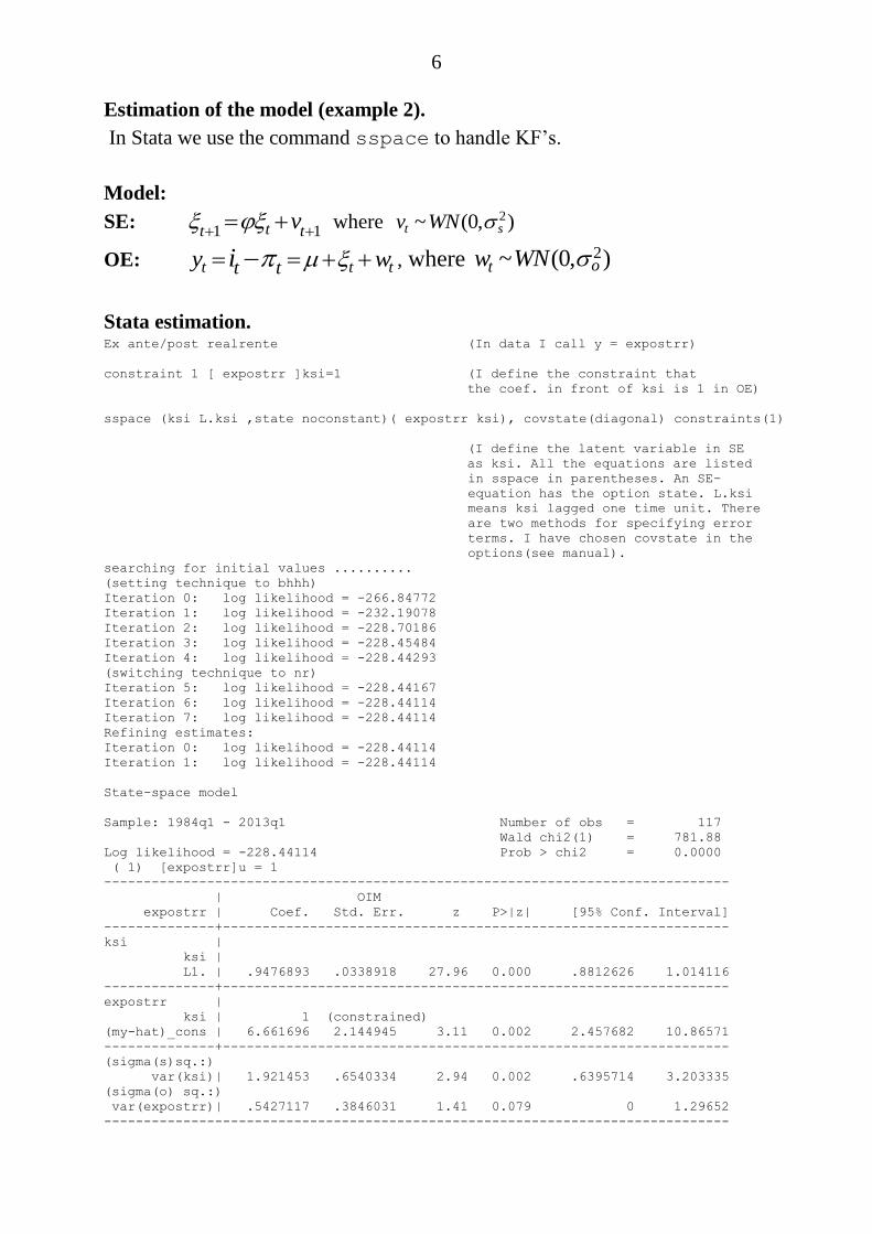
Estimation of the model (example 2).

In Stata we use the command sspace to handle KF’s.

Model:

SE: 1 1tt t

v where 2~ (0, )t sv WN

OE: t t tt ty wi , where 2~ (0, )otw WN

Stata estimation. Ex ante/post realrente (In data I call y = expostrr)

constraint 1 [ expostrr ]ksi=1 (I define the constraint that

the coef. in front of ksi is 1 in OE)

sspace (ksi L.ksi ,state noconstant)( expostrr ksi), covstate(diagonal) constraints(1)

(I define the latent variable in SE

as ksi. All the equations are listed

in sspace in parentheses. An SE-

equation has the option state. L.ksi

means ksi lagged one time unit. There

are two methods for specifying error

terms. I have chosen covstate in the

options(see manual).

searching for initial values ..........

(setting technique to bhhh)

Iteration 0: log likelihood = -266.84772





(switching technique to nr)




Refining estimates:



State-space model

Sample: 1984q1 - 2013q1 Number of obs = 117

Wald chi2(1) = 781.88

Log likelihood = -228.44114 Prob > chi2 = 0.0000

( 1) [expostrr]u = 1

-------------------------------------------------------------------------------

| OIM

expostrr | Coef. Std. Err. z P>|z| [95% Conf. Interval]

--------------+----------------------------------------------------------------

ksi |

ksi |

L1. | .9476893 .0338918 27.96 0.000 .8812626 1.014116

--------------+----------------------------------------------------------------

expostrr |

ksi | 1 (constrained)

(my-hat)_cons | 6.661696 2.144945 3.11 0.002 2.457682 10.86571

--------------+----------------------------------------------------------------

(sigma(s)sq.:)

var(ksi)| 1.921453 .6540334 2.94 0.002 .6395714 3.203335

(sigma(o) sq.:)

var(expostrr)| .5427117 .3846031 1.41 0.079 0 1.29652

-------------------------------------------------------------------------------

7

Note: Tests of variances against zero are one sided, and the two-sided confidence

intervals are truncated at zero.

Some interpretation of output:

It turns out that the Kalman-filter estimes to 0.95 which indicates

almost random walk (RW).

The variances, 2 2,s o were estimated as 1.9 and 0.5 respectively,

indicating relatively high volatility in the ex ante r.i.r. (too high for the

approximate RW to be interpreted reasonably as a locally constant trend

RW.

It is tempting to interpret the fact that 2ˆo is relatively small as a tendency

that ex ante r.i.r. follows (the observable) ex post r.i.r. rather tightly – i.e.,

that much of the variation in ty has been “taken over” by t .

In other words: The results seem to indicate a co-integration relationship

between ex post and ex ante r.i.r.

Using the sspace post-estimation command predict, we can get the

forward one-step-ahead predictions (the filterings) of ksi, and the backwards

smoothing predictions of ksi from the total series:

predict exfilter1,states smethod(filter) equation(ksi)

predict exsmooth1,states smethod(smooth) equation(ksi)

To list some values to compare with ty expostrr, I need to add ˆ 6.6617 to

the predicted ksi’s:

. gen rrfilter1= exfilter1+6.6617

(25 missing values generated)

. gen rrsmooth1= exsmooth1+6.6617


list t expostrr rrfilter1 rrsmooth1 if tin(2009q1,2013q1), compress noobs

+--------------------------------+

| t exp~r rrf~1 rrs~1 |

|--------------------------------|

| 2009q1 6.1 5.8 5.68 |

| 2009q2 5 5.16 5.18 |

| 2009q3 6 5.86 5.35 |

8

| 2009q4 3 3.55 3.09 |

| 2010q1 .6 1.19 1.13 |

|--------------------------------|

| 2010q2 .9 1.01 1.14 |

| 2010q3 2.5 2.27 2.01 |

| 2010q4 .7 1.04 1.03 |

| 2011q1 1.2 1.23 1.27 |

| 2011q2 1.6 1.58 1.73 |

|--------------------------------|

| 2011q3 3.1 2.86 2.66 |

| 2011q4 1.8 2.04 1.95 |

| 2012q1 1.6 1.73 1.77 |

| 2012q2 2.2 2.16 2.21 |

| 2012q3 3.3 3.13 2.68 |

|--------------------------------|

| 2012q4 .3 .872 .817 |

| 2013q1 .8 .871 .871 |

+--------------------------------+

Using the twoway command graph combine, I can produce the following

graphs,

One can filter forwards and backwards

Forward filtering (called filtering) filters, updates, and predicts next

period ( 1t ) every time a new observation ty is available.

observed

filtered

smoothed

51

01

52

0

1992q3 1993q1 1993q3 1994q1 1994q3t

expostrr RIR est ex ante (filtered)

RIR est ex ante smoothed

1992q3 -1994q3

02

46

2009q1 2010q1 2011q1 2012q1 2013q1t

expostrr RIR est ex ante (filtered)

RIR est ex ante smoothed

2009q1 - 2013q1

Real I.R. expost, filtered (ex ante), and smoothed (ex ante)

9

Backwards filtering (called smoothing)) is used for the complete data set,

1 2, , , Ty y y , and updates earlier predictions by recursive calculations

backwards from time T.

Forwards filtering

SE: 1 1

), 0,1,2, dim(t tt tr rrF v t

OE: )' ' , 1,2, dim( tt t t tn rn kny A x H w t y

Example 2 r.i.r:

1n r t t ty i

) ( ))( (ex ante r.i.r.e et t t t tEi E i

SE: 1 1tt tv where 2~ (0, )t sv WN ( 1 og r F )

OE: t t tt ty wi , where 2~ (0, )t ow WN

( 1 og 1tA x H )

2sQ , 2

oR

Time period t:

Step 1 – before ty is observed:

Info from period t – 1:

1 1 2

1

.2

1| 1

.2

| 1 | 1 | 1 | 1 | 1

, ,ˆ ( ) ~ 1 1

ˆ ˆ ˆ( ) ~1 1

t t t

t

Ex

t tt t

Ex

t tt t t t t t t t t t

D y y

D

E D

P MSE E p

.2

| 1 | 1 | 1ˆ ˆˆ

Ex

tt t t t t ty A x H

.2

21 | 1 | 1| 1

ˆEx

ot t t t tt tMSE H P H R py

10

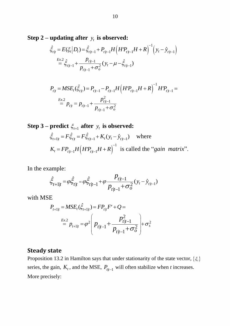
Step 2 – updating after ty is observed:

1

| | 1 | 1 | 1 | 1

.2 | 1

| 1 | 12| 1

ˆ ˆ ˆ( )

ˆ ˆ ( )

t t tt t t t t t t t t t

Ex t ttt t t t

ot t

E D P H H P H R y y

py

p

1

| | | 1 | 1 | 1 | 1

2.2 | 1

| | 1 2| 1

ˆ( )

tt t t t t t t t t t t t

Ex t tt t t t

ot t

P MSE P P H H P H R H P

pp p

p

Step 3 – predict 1t

after ty is observed:

1| | | 1 | 1

ˆ ˆ ˆ ˆ( )t tt t t t t t t tF F K y y

where

1

| 1 | 1t t t t tK FP H H P H R

is called the “gain matrix”.

In the example:

| 1

| 11| | | 1 2

| 1

ˆ( )ˆ ˆ ˆt t t

t tt t t t t t

ot t

y yp

p

with MSE

1| 1| |

.22 2

1|

2| 1

| 1 2| 1

ˆ( )

tt t t t t t

Ex

st t

t tt t

ot t

P MSE FP F Q

pp

pp

Steady state Proposition 13.2 in Hamilton says that under stationarity of the state vector, t

series, the gain, tK , and the MSE, | 1t t

P

will often stabilize when t increases.

More precisely:

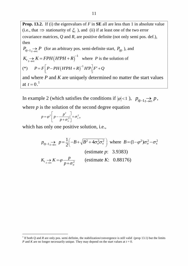
11

Prop. 13.2. If (i) the eigenvalues of F in SE all are less than 1 in absolute value

(i.e., that stationarity of t ), and (ii) if at least one of the two error

covariance matrices, Q and R, are positive definite (not only semi pos. def.),

then

| 1t t tP P

(for an arbitrary pos. semi-definite start,

1|0P ), and

1

t tK K FPH H PH R

where P is the solution of

(*) 1

P F P PH H PH R H P F Q

and where P and K are uniquely determined no matter the start values

at 0t .1

In example 2 (which satisfies the conditions if 1 ), | 1t t t

p p ,

where p is the solution of the second degree equation

2

2 2

2 s

o

pp p

p

,

which has only one positive solution, i.e.,

2 2 2 2 2 2| 1

14 where (1 )

2 o s o st t tp p B B B

(estimate p: 3.9383)

2t to

pK K

p

(estimate K: 0.88176)

1 If both Q and R are only pos. semi definite, the stabilization/convergence is still valid (prop 13.1) but the limits

P and K are no longer necessarily unique. They may depend on the start values at t = 0.

12

Stable updating relations in example 2.

| 1 | 1

ˆˆ 6.6617t t t t

y

| | 1 | 1

0.9304ˆ ˆ ˆ( )t t t t t tt yy

1| | | 1 | 1

| 1 | 1 (0.9477) (0.88176)

ˆ ˆ ˆ ˆ( )

ˆ ˆ( )

tt t t t t t t t

tt t t t

K y y

y y

1|

ˆ( ) 3.9383t t tMSE p

Example 3 Local linear trend (structural time series) Consider the ln BNP data.

We want to model the trend. There are many ways to model trends. One way is

Harvey’s local linear trend model as an example of his structural time series

approach..

Let lnt ty BNP . We imagine that that ty can be decomposed

(1) t t ty w

12.2

12.4

12.6

12.8

13

ln B

NP

FN

1980q1 1990q1 2000q1 2010q1t

ln(BNP)

13

where t is the trend component and tw an error. Both and t tw are latent

random variables.

One possibility is the “locally constant” trend model where

(2) 1t t tv where 2~ (0, )t vv WN and independent of

1 2 1, , , , ,t t t ty y

This implies that 0 1t tv v is a random walk. However, t behaves

as a trend only if the variance of the error tv is substantially smaller than

2 = var( )w tw in (1).

It is in this sense we call t “locally constant”.

This model is well suited for estimation by the KF.

The “locally linear” trend model is an extension of this: Adding a constant, b, to

(2) we get

(3) 1 1 0 11 1t t t t tb v bt v v

i.e., a random walk with a deterministic trend component (called a “random

walk with drift”). However, the rate of increase of the deterministic part is fixed

in this model. It is natural to think that the rate of increase may vary randomly

although slowly. This we can achieve by replacing b by a random rate of

increase, t , where 1 2t t tv with 2

2

2 ~ (0, )t vv WN and where

2

2

2var( )v tv is small relatively to var( )tw , i.e., a “locally constant” rate of

increase. So the locally linear trend model is specified as the following state

space model.

OE: t t ty w

SE: 1 1 1

1 2

t t t t

t t t

v

v

14

or in matrix form

SE: 1 1

1 2

1 1

0 1

t t t

t

t t t

v

v

OE: 1,0t t ty w

The KF will provide one-step-ahead predictions (filtering), or full-sample

predictions (smoothing) for the 't s , and estimates for the variance parameters,

1 2

2 2 2, ,w v v , where the two last ones should be substantially smaller than 2

w for

t to behave like a trend.

Note, in passing, that this model implies that ~ (2)ty I (unless 2var( ) 0tv ),

since 1 1t t t t t ty w v w , i.e., a random walk, and only 2

ty is

stationary. If, however, 2var( ) 0tv , the t becomes a constant, and we are

back to the case where ty is a random walk with drift, i.e., I(1).

In the following Stata sspace command, I call the two state equation for “s1”

and “s2”, and the observation equation for “y”. The restrictions are

. constraint 1 [s1]L.s1=1



. constraint 4 [y]s1=1

The KF command

. sspace (s1 L.s1 L.s2,state noconstant) (s2 L.s2,state noconstant) (y s1,noconst),

constraints(1/4)

----- Iteration output omitted (22 iterations)----

State-space model


Log likelihood = 442.9024

( 1) [s1]L.s1 = 1

( 2) [s1]L.s2 = 1

( 3) [s2]L.s2 = 1

( 4) [y]s1 = 1

------------------------------------------------------------------------------

| OIM

15

y | Coef. Std. Err. z P>|z| [95% Conf. Interval]

-------------+----------------------------------------------------------------

s1 |

s1 |

L1. | 1 (constrained)

|

s2 |


-------------+----------------------------------------------------------------

s2 |

s2 |


-------------+----------------------------------------------------------------

y |

s1 | 1 (constrained)

-------------+----------------------------------------------------------------

var(s1)| 2.35e-17 . . . . .

var(s2)| 5.20e-06 1.55e-06 3.36 0.000 2.17e-06 8.23e-06

var(y)| .0000433 6.07e-06 7.13 0.000 .0000314 .0000552

------------------------------------------------------------------------------

Note: Model is not stationary.



We notice that state variances are substantially smaller than the observation

error variance. The 1var( ) 0tv , but the rate of increase appears to be random

2var( ) 0tv .

We obtain the residuals ˆtw for ty by by the predict post-estimation

command:

. predict resy,resid

. corrgram resy

-1 0 1 -1 0 1

LAG AC PAC Q Prob>Q [Autocorrelation] [Partial Autocor]

-------------------------------------------------------------------------------

1 -0.0220 -0.0221 .06932 0.7923 | |

2 -0.0123 -0.0133 .09119 0.9554 | |

3 0.0427 0.0422 .35532 0.9493 | |

4 0.0564 0.0586 .82032 0.9357 | |

5 0.0021 0.0054 .82097 0.9757 | |

6 -0.0944 -0.0961 2.1427 0.9061 | |

7 0.0108 0.0021 2.1602 0.9504 | |

8 -0.1904 -0.1976 7.6215 0.4713 -| -|

9 0.0701 0.0714 8.368 0.4975 | |

10 -0.1088 -0.1094 10.177 0.4251 | |

11 -0.0154 0.0025 10.214 0.5113 | |

12 -0.0417 -0.0497 10.484 0.5735 | |

13 -0.0415 -0.0394 10.754 0.6314 | |

14 0.0760 0.0505 11.666 0.6331 | |

15 -0.1159 -0.1082 13.8 0.5407 | |

16 0.0067 -0.0564 13.808 0.6130 | |

17 -0.0850 -0.0851 14.976 0.5972 | |

18 -0.0465 -0.1298 15.327 0.6394 | -|

19 -0.0403 -0.0564 15.594 0.6841 | |

20 -0.0514 -0.0897 16.031 0.7147 | |

21 -0.0304 -0.0828 16.185 0.7591 | |

22 -0.2384 -0.3108 25.763 0.2620 -| --|

23 0.1235 -0.0032 28.357 0.2026 | |

16

24 0.0157 -0.0352 28.399 0.2436 | |

25 0.0450 -0.0277 28.749 0.2745 | |

26 -0.0254 -0.0981 28.862 0.3174 | |

27 0.1325 0.1345 31.951 0.2339 |- |-

28 0.0795 -0.0179 33.074 0.2330 | |

29 0.0394 0.0670 33.351 0.2638 | |

30 0.0917 -0.0450 34.87 0.2474 | |

31 -0.1131 -0.0599 37.203 0.2050 | |

32 0.1133 0.0703 39.567 0.1680 | |

33 -0.0503 -0.1019 40.037 0.1862 | |

34 -0.0453 -0.1792 40.422 0.2077 | -|

35 -0.0146 -0.0474 40.462 0.2418 | |

36 -0.0687 -0.1421 41.365 0.2479 | -|

37 0.0970 0.0063 43.181 0.2241 | |

38 -0.0745 -0.2018 44.264 0.2242 | -|

39 0.1188 0.0795 47.04 0.1765 | |

40 0.0945 0.1534 48.816 0.1599 | |-

No strong evidence against tw being WN.

We get the smoothed prediction of the trend ˆt by the predict as well:

. predict ysmooth,xb smethod(smooth)

and the plot

. tsline y ysmooth if t>=tq(2005q1)

12.7

51

2.8

12.8

51

2.9

12.9

5

13

2005q1 2007q1 2009q1 2011q1 2013q1t

ln BNP FN xb prediction, y, smooth

lnBNP with local linear trend - smoothed

17

Note. This is an example that the KF handles a non-stationary dynamic model

with standard asymptotic normal inference theory. There are general results in

the literature that says that this is the case when the parameters determining the

non-stationary part of the model are all specified as known (i.e., the case here).

As the cointegration theory will show, this is not always the case when some

parameters of the non-stationary part are unknown and must be estimated –

especially when some of the eigenvalues of F in the SE lie exactly on the unit

circle. Then the inference theory must be modified (i.e., the Søren Johansen

theory). In such cases the Stata sspace command will refuse to work.

On the other hand, sspace sometimes works well in other non-stationary cases

with unknown parameters for the non-stationary part of the model as long as

there are no eigenvalues on the unit circle. The following example taken from

the recommendable, R.H. Shumway and D.S. Stoffer, “Time Series Analysis and

Its Applications”, Springer 2000, is an illustration.

Example 4 Johnson & Johnson Quarterly Sales Data

05

10

15

JJ q

uart

erl

y e

arn

ings

1960q1 1965q1 1970q1 1975q1 1980q1time

Johnson & Johnson Quarterly Earnings

18

These data are highly non-stationary and have strong seasonal effects. They also

appear to show an increasing volatility.

It turns out, as Shumway and Stoffer (S&S) point out, that these data are hard to

bring to stationarity by differencing and transformations (log or n-th root

transformations). So they decide to analyze the data using a wrong model (with

the error terms failing to be white noise), but where the KF give meaningful

results. They use a different estimation approach than provided by sspace.

But even sspace can handle wrong models to a certain degree by the quasi

likelihood method (QML),, which turns out to provide quite similar results as in

S&S.

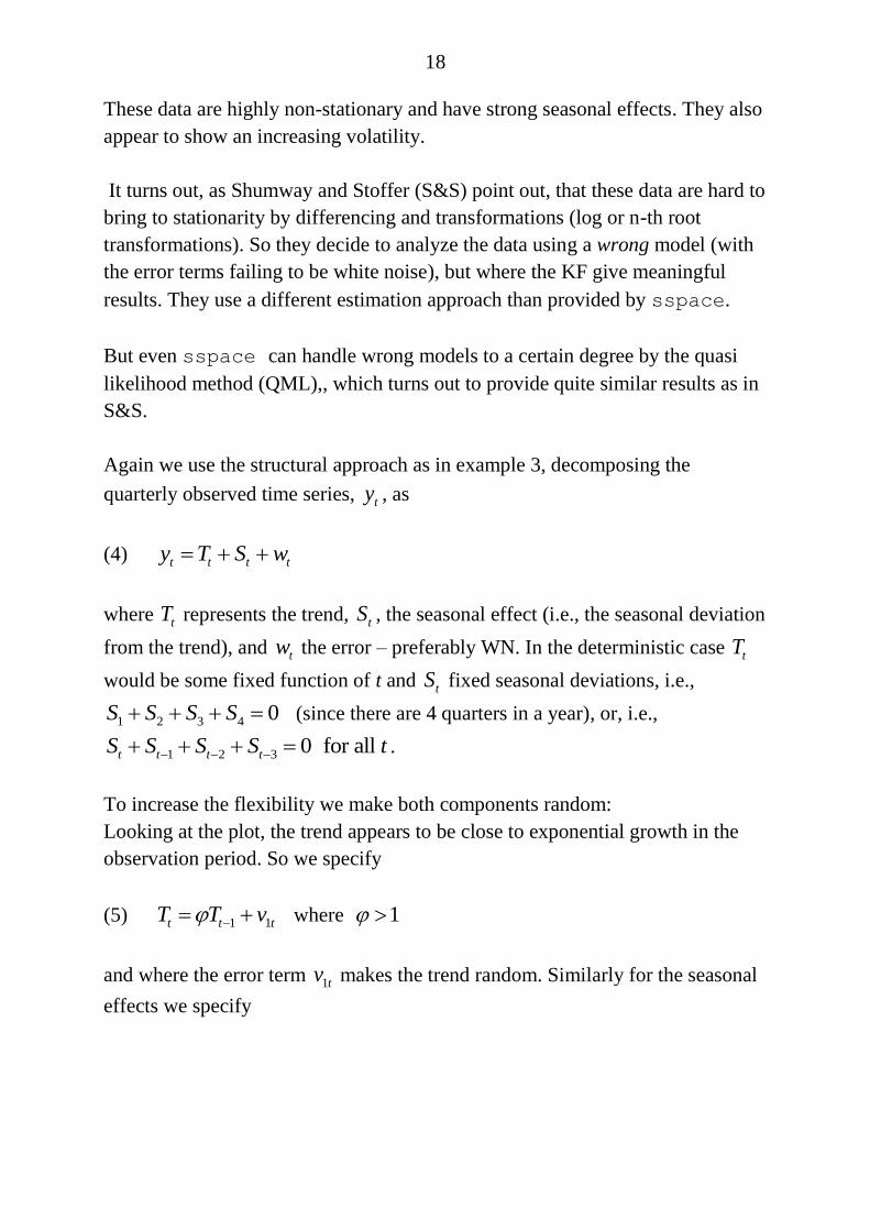
Again we use the structural approach as in example 3, decomposing the

quarterly observed time series, ty , as

(4) t t t ty T S w

where tT represents the trend, tS , the seasonal effect (i.e., the seasonal deviation

from the trend), and tw the error – preferably WN. In the deterministic case tT

would be some fixed function of t and tS fixed seasonal deviations, i.e.,

1 2 3 4 0S S S S (since there are 4 quarters in a year), or, i.e.,

1 2 3 0 for all t t t tS S S S t .

To increase the flexibility we make both components random:

Looking at the plot, the trend appears to be close to exponential growth in the

observation period. So we specify

(5) 1 1t t tT T v where 1

and where the error term 1tv makes the trend random. Similarly for the seasonal

effects we specify

19

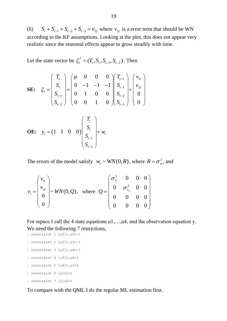
(6) 1 2 3 2t t t t tS S S S v where 2tv is a error term that should be WN

according to the KF assumptions. Looking at the plot, this does not appear very

realistic since the seasonal effects appear to grow steadily with time.

Let the state vector be 1 2( , , , )t t t t tT S S S

. Then

SE:

1 1

1 2

1 2

2 3

0 0 0

0 1 1 1

0 1 0 0 0

0 0 1 0 0

t t t

t t t

t

t t

t t

T T v

S S v

S S

S S

OE: 1

2

1 1 0 0

t

t

t t

t

t

T

Sy w

S

S

The errors of the model satisfy ~ (0, )tw WN R , where 2

wR , and

1

2~ (0, )

0

0

t

t

t

v

vv WN Q

, where

1

2

2

2

0 0 0

0 0 0

0 0 0 0

0 0 0 0

v

vQ

For sspace I call the 4 state equations u1,…,u4, and the observation equation y.

We need the following 7 restrictions, . constraint 1 [u2]L.u2=-1

. constraint 2 [u2]L.u3=-1

. constraint 3 [u2]L.u4=-1

. constraint 4 [u3]L.u2=1

. constraint 5 [u4]L.u3=1

. constraint 6 [y]u1=1

. constraint 7 [y]u2=1

To compare with the QML I do the regular ML estimation first.

20

. sspace (u1 L.u1,state noconst) (u2 L.u2 L.u3 L.u4,state noconstant) (u3

L.u2,state noerror noconst) (u4 L.u3, state noerror noconst) (y u1 u2,

noconst),covstate(diagonal) constraints(1/7)

------ Iteration output omitted -----

State-space model


Wald chi2(1) = 165386.98


( 1) [u2]L.u2 = -1

( 2) [u2]L.u3 = -1

( 3) [u2]L.u4 = -1

( 4) [u3]L.u2 = 1

( 5) [u4]L.u3 = 1

( 6) [y]u1 = 1

( 7) [y]u2 = 1

------------------------------------------------------------------------------

| OIM


-------------+----------------------------------------------------------------

u1 |

u1 |

L1. | 1.035097 .0025452 406.68 0.000 1.030108 1.040085

-------------+----------------------------------------------------------------

u2 |

u2 |

L1. | -1 (constrained)

|

u3 |


|

u4 |


-------------+----------------------------------------------------------------

u3 |

u2 |


-------------+----------------------------------------------------------------

u4 |

u3 |


-------------+----------------------------------------------------------------

y |

u1 | 1 (constrained)


-------------+----------------------------------------------------------------

var(u1)| .0196384 .0061475 3.19 0.001 .0075896 .0316873

var(u2)| .0503249 .0110313 4.56 0.000 .028704 .0719458

var(y)| 2.84e-15 . . . . .

------------------------------------------------------------------------------




I also want out-of-sample predictions for four years (the sample period is

1960q1 – 1980q4). So

. tsappend, add(16)

21

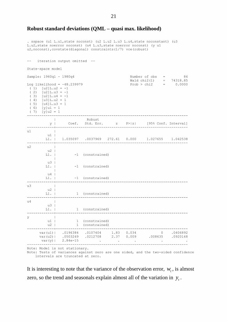
Robust standard deviations (QML – quasi max. likelihood)

. sspace (u1 L.u1,state noconst) (u2 L.u2 L.u3 L.u4,state noconstant) (u3

L.u2,state noerror noconst) (u4 L.u3,state noerror noconst) (y u1

u2,noconst),covstate(diagonal) constraints(1/7) vce(robust)

-- iteration output omitted --

State-space model


Wald chi2(1) = 74318.85


( 1) [u2]L.u2 = -1

( 2) [u2]L.u3 = -1

( 3) [u2]L.u4 = -1

( 4) [u3]L.u2 = 1

( 5) [u4]L.u3 = 1

( 6) [y]u1 = 1

( 7) [y]u2 = 1

------------------------------------------------------------------------------

| Robust


-------------+----------------------------------------------------------------

u1 |

u1 |

L1. | 1.035097 .0037969 272.61 0.000 1.027655 1.042538

-------------+----------------------------------------------------------------

u2 |

u2 |


|

u3 |


|

u4 |


-------------+----------------------------------------------------------------

u3 |

u2 |


-------------+----------------------------------------------------------------

u4 |

u3 |


-------------+----------------------------------------------------------------

y |



-------------+----------------------------------------------------------------

var(u1)| .0196384 .0107404 1.83 0.034 0 .0406892

var(u2)| .0503249 .0212708 2.37 0.009 .008635 .0920148

var(y)| 2.84e-15 . . . . .

------------------------------------------------------------------------------




It is interesting to note that the variance of the observation error, tw , is almost

zero, so the trend and seasonals explain almost all of the variation in ty .

22

The residuals of OE: . predict resy,resid

. tsline resy if e(sample)

Clearly far from WN.

Now forecasts and trend (including “root mean square errors” for the forecasts

. predict f_y,dynamic(tq(1980q4)) rmse(rmse_f_y)

. predict trend if e(sample), states smethod(smooth) equation(u1)

-1.5

-1-.

50

.51

resid

ua

ls, y, o

ne

ste

p

1960q1 1965q1 1970q1 1975q1 1980q1time

The observation residuals

23

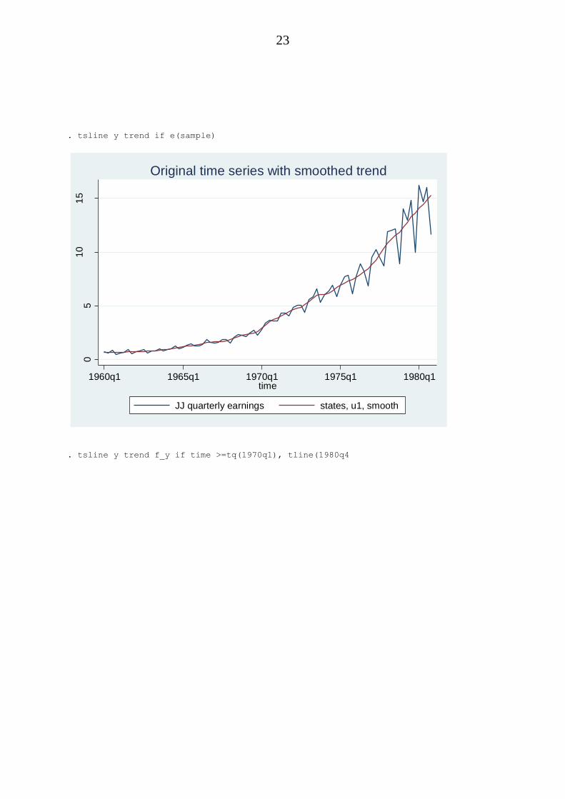
. tsline y trend if e(sample)

. tsline y trend f_y if time >=tq(1970q1), tline(1980q4

05

10

15

1960q1 1965q1 1970q1 1975q1 1980q1time

JJ quarterly earnings states, u1, smooth

Original time series with smoothed trend

24

Partial prediction uncertainty from root MSE based on error variation only

. gen upmse =f_y+invnorm(0.975)* rmse_f_y if time >=tq(1981q1)


. gen dnmse =f_y+invnorm(0.025)* rmse_f_y if time >=tq(1981q1)


. tsline y trend f_y dnmse upmse if time >=tq(1970q1), tline(1980q4)

01

02

03

0

1970q1 1975q1 1980q1 1985q1time


xb prediction, y, dynamic(tq(1980q4))

Out-of-sample forecasts

25

Prediction uncertainty grows with t.

Further details of the forecasts can be achieved by the forecast command.

01

02

03

0

1970q1 1975q1 1980q1 1985q1time


xb prediction, y, dynamic(tq(1980q4)) dnmse

upmse

(estimation uncertainty ignored)

Out-of sample forecasts with prediction intervals due to error

1. Introduction to the Kalman filter - Universitetet i oslo · 7 Note: Tests of variances against...

Documents

Transcript of 1. Introduction to the Kalman filter - Universitetet i oslo · 7 Note: Tests of variances against...