1 INTRODUCTION TO MULTILEVEL ANALYSIS · 1 INTRODUCTION TO MULTILEVEL ANALYSIS ... The first...
84
1 1 INTRODUCTION TO MULTILEVEL ANALYSIS Social research regularly involves problems that investigate the relationship between individual and society. The general concept is that individuals interact with the social contexts to which they belong, that individual persons are influenced by the social groups or contexts to which they belong, and that those groups are in turn influenced by the individuals who make up that group. The individuals and the social groups are conceptualized as a hierarchical system of individuals nested within groups, with individuals and groups defined at separate levels of this hierarchical system. Naturally, such systems can be observed at different hierarchical levels, and variables may be defined at each level. This leads to research into the relationships between variables characterizing individuals and variables characterizing groups, a kind of research that is generally referred to as ‘multilevel research’. In multilevel research, the data structure in the population is hierarchical, and the sample data are a sample from this hierarchical population. Thus, in educational research, the population consists of schools and pupils within these schools, and the sampling procedure often proceeds in two stages: first, we take a sample of schools, and next we take a sample of pupils within each school. Of course, in real research one may have a convenience sample at either level, or one may decide not to sample pupils but to study all available pupils in the sample of schools. Nevertheless, one should keep firmly in mind that the central statistical model in multilevel analysis is one of successive sampling from each level of a hierarchical population. In this example, pupils are nested within schools. Other examples are cross-national studies where the individuals are nested within their national units, organizational research with individuals nested within departments within organizations, family research with family members within families and methodological research into interviewer effects with respondents nested within interviewers. Less obvious applications of multilevel models are longitudinal research and growth curve research, where a series of several distinct observations are viewed as nested within individuals and meta-analysis where the subjects are nested within different studies. For simplicity, this book describes the multilevel models mostly in terms of individuals nested within groups, but note that the models apply to a much larger class of analysis problems. 1.1 AGGREGATION AND DISAGGREGATION In multilevel research, variables can be defined at any level of the hierarchy. Some of these variables may be measured directly at their ‘own’ natural level; for example, at the school level we may measure school size and denomination, and at the pupil level intelligence and school success. In addition, we may move variables from one level to another by aggregation or disaggregation. Aggregation means that the variables at a lower level are moved to a higher level, for instance, by assigning to the schools the school mean of the pupils' intelligence scores. Disaggregation means moving variables to a lower level, for instance by assigning to all pupils in the schools a variable that indicates the denomination of the school they belong to.
Transcript of 1 INTRODUCTION TO MULTILEVEL ANALYSIS · 1 INTRODUCTION TO MULTILEVEL ANALYSIS ... The first...

1
1
INTRODUCTION TO MULTILEVEL ANALYSIS Social research regularly involves problems that investigate the relationship between individual and society. The general concept is that individuals interact with the social contexts to which they belong, that individual persons are influenced by the social groups or contexts to which they belong, and that those groups are in turn influenced by the individuals who make up that group. The individuals and the social groups are conceptualized as a hierarchical system of individuals nested within groups, with individuals and groups defined at separate levels of this hierarchical system. Naturally, such systems can be observed at different hierarchical levels, and variables may be defined at each level. This leads to research into the relationships between variables characterizing individuals and variables characterizing groups, a kind of research that is generally referred to as ‘multilevel research’. In multilevel research, the data structure in the population is hierarchical, and the sample data are a sample from this hierarchical population. Thus, in educational research, the population consists of schools and pupils within these schools, and the sampling procedure often proceeds in two stages: first, we take a sample of schools, and next we take a sample of pupils within each school. Of course, in real research one may have a convenience sample at either level, or one may decide not to sample pupils but to study all available pupils in the sample of schools. Nevertheless, one should keep firmly in mind that the central statistical model in multilevel analysis is one of successive sampling from each level of a hierarchical population. In this example, pupils are nested within schools. Other examples are cross-national studies where the individuals are nested within their national units, organizational research with individuals nested within departments within organizations, family research with family members within families and methodological research into interviewer effects with respondents nested within interviewers. Less obvious applications of multilevel models are longitudinal research and growth curve research, where a series of several distinct observations are viewed as nested within individuals and meta-analysis where the subjects are nested within different studies. For simplicity, this book describes the multilevel models mostly in terms of individuals nested within groups, but note that the models apply to a much larger class of analysis problems. 1.1 AGGREGATION AND DISAGGREGATION In multilevel research, variables can be defined at any level of the hierarchy. Some of these variables may be measured directly at their ‘own’ natural level; for example, at the school level we may measure school size and denomination, and at the pupil level intelligence and school success. In addition, we may move variables from one level to another by aggregation or disaggregation. Aggregation means that the variables at a lower level are moved to a higher level, for instance, by assigning to the schools the school mean of the pupils' intelligence scores. Disaggregation means moving variables to a lower level, for instance by assigning to all pupils in the schools a variable that indicates the denomination of the school they belong to.

Introduction
2
The lowest level (level 1) is usually defined by the individuals. However, this is not always the case. Galtung (1969), for instance, defines roles within individuals as the lowest level, and in longitudinal designs, repeated measures within individuals are the lowest level. At each level in the hierarchy, we may have several types of variables. The distinctions made in the following are based on the typology offered by Lazarsfeld and Menzel (1961), with some simplifications. In our typology, we distinguish between global, structural and contextual variables. Global variables are variables that refer only to the level at which they are defined, without reference to other units or levels. A pupil's intelligence or gender would be a global variable at the pupil level. School size would be a global variable at the school level. A global variable is measured at the level at which that variable actually exists. Structural variables are operationalized by referring to the sub-units at a lower level. They are constructed from variables at a lower level, for example, in defining the school variable ‘mean intelligence’ as the mean of the intelligence scores of the pupils in that school. Using the mean of a lower-level variable as an explanatory variable at a higher level is a common procedure in multilevel analysis. Other functions of the lower-level variables are less common, but may also be valuable. For instance, using the standard deviation of a lower-level variable as an explanatory variable at a higher level could be used to test hypotheses about the effect of group heterogeneity on the outcome variable. Klein and Kozlowski (2000) refer to such variables as configural variables, and stress the importance of capturing the pattern of individual variation in a group. Their examples also emphasize the use of other functions than the mean of individual scores to reflect group characteristics. It is clear that constructing a structural variable from the lower-level data involves aggregation. Contextual variables, on the other hand, refer to the super-units; all units at the lower level receive the value of a variable for the super-unit to which they belong at the higher level. For instance, we can assign to all pupils in a school the school size, or the mean intelligence, as a pupil level variable. This is called disaggregation; data on higher-level units are disaggregated into data on a larger number of lower-level units. The resulting variable is called a contextual variable, because it refers to the higher-level context of the units we are investigating. In order to analyze multilevel models, it is not important to assign each variable to its proper place in the typology. The benefit of the scheme is conceptual; it makes clear to which level a measurement properly belongs. Historically, multilevel problems have led to analysis approaches that moved all variables by aggregation or disaggregation to one single level of interest followed by an ordinary multiple regression, analysis of variance, or some other ‘standard’ analysis method. However, analyzing variables from different levels at one single common level is inadequate, and leads to two distinct types of problems. The first problem is statistical. If data are aggregated, the result is that different data values from many sub-units are combined into fewer values for fewer higher-level units. As a result, much information is lost, and the statistical analysis loses power. On the other hand, if data are disaggregated, the result is that a few data values from a small number of super-units are ‘blown up’ into many more values for a much larger number of sub-units. Ordinary statistical tests treat all these disaggregated data values as independent information from the much larger sample of sub-units. The proper sample size for these variables is of course the number of higher-level units. Using the larger number of disaggregated cases for the sample size leads to significance tests that reject the null-hypothesis far more often than the nominal alpha level suggests. In other words: investigators come up with many ‘significant’ results that are totally spurious. The second problem is conceptual. If the analyst is not very careful in the interpretation of the results, s/he may commit the fallacy of the wrong level, which consists of analyzing the

Multilevel Analysis; Techniques and Applications 3
data at one level, and formulating conclusions at another level. Probably the best-known fallacy is the ecological fallacy, which is interpreting aggregated data at the individual level. It is also known as the ‘Robinson effect’ after Robinson (1950). Robinson presents aggregated data describing the relationship between the percentage of blacks and the illiteracy level in nine geographic regions in 1930. The ecological correlation, that is, the correlation between the aggregated variables at the region level is 0.95. In contrast, the individual-level correlation between these global variables is 0.20. Robinson concludes that in practice an ecological correlation is almost certainly not equal to its corresponding individual-level correlation. For a statistical explanation, see Robinson (1950) or Kreft and de Leeuw (1987). Formulating inferences at a higher level based on analyses performed at a lower level is just as misleading. This fallacy is known as the atomistic fallacy. A related but different fallacy is known as ‘Simpson's Paradox’ (see Lindley & Novick, 1981). Simpson's paradox refers to the problem that completely erroneous conclusions may be drawn if grouped data, drawn from heterogeneous populations, are collapsed and analyzed as if they came from a single homogeneous population. An extensive typology of such fallacies is given by Alker (1969). When aggregated data are the only available data, King (1997) presents some procedures that make it possible to estimate the corresponding individual relationships without committing an ecological fallacy. A better way to look at multilevel data is to realize that there is not one ‘proper’ level at which the data should be analyzed. Rather, all levels present in the data are important in their own way. This becomes clear when we investigate cross-level hypotheses, or multilevel problems. A multilevel problem is a problem that concerns the relationships between variables that are measured at a number of different hierarchical levels. For example, a common question is how a number of individual and group variables influence one single individual outcome variable. Typically, some of the higher-level explanatory variables may be the aggregated group means of lower-level individual variables. The goal of the analysis is to determine the direct effect of individual and group level explanatory variables, and to determine if the explanatory variables at the group level serve as moderators of individual-level relationships. If group level variables moderate lower-level relationships, this shows up as a statistical interaction between explanatory variables from different levels. In the past, such data were usually analyzed using conventional multiple regression analysis with one dependent variable at the lowest (individual) level and a collection of explanatory variables from all available levels (cf. Boyd & Iversen, 1979; Roberts & Burstein, 1980; van den Eeden & Hüttner, 1982). Since this approach analyzes all available data at one single level, it suffers from all of the conceptual and statistical problems mentioned above. 1.2 WHY DO WE NEED SPECIAL MULTILEVEL ANALYSIS TECHNIQUES? A multilevel problem concerns a population with a hierarchical structure. A sample from such a population can be described as a multistage sample: first, we take a sample of units from the higher level (e.g., schools), and next we sample the sub-units from the available units (e.g., we sample pupils from the schools). In such samples, the individual observations are in general not completely independent. For instance, pupils in the same school tend to be similar to each other, because of selection processes (for instance, some schools may attract pupils from higher social economic status (SES) levels, while others attract lower SES pupils) and because of the common history the pupils share by going to the same school. As a result, the average correlation (expressed in the so-called intraclass correlation) between variables measured on pupils from the same school will be higher than the average correlation between variables measured on pupils from different schools. Standard statistical tests lean heavily on

Introduction
4
the assumption of independence of the observations. If this assumption is violated (and in multilevel data this is almost always the case) the estimates of the standard errors of conventional statistical tests are much too small, and this results in many spuriously ‘significant’ results. The effect is generally not negligible, small dependencies in combination with large group sizes still result in large biases in the standard errors. The strong biases that may be the effect of violation of the assumption of independent observations made in standard statistical tests has been known for a long time (Walsh, 1947) and are still a very important assumption to check in statistical analyses (Stevens, 2009). The problem of dependencies between individual observations also occurs in survey research, if the sample is not taken at random but cluster sampling from geographical areas is used instead. For similar reasons as in the school example given above, respondents from the same geographical area will be more similar to each other than respondents from different geographical areas are. This leads again to estimates for standard errors that are too small and produce spurious ‘significant’ results. In survey research, this effect of cluster sampling is well known (cf. Kish, 1965, 1987). It is called a ‘design effect’, and various methods are used to deal with it. A convenient correction procedure is to compute the standard errors by ordinary analysis methods, estimate the intraclass correlation between respondents within clusters, and finally employ a correction formula to the standard errors. A correction described by Kish (1965: p. 259) corrects the sampling variance using
( )( )1 1eff clusv v n ρ= + − , where veff is the effective sampling variance, v is the sampling variance calculated by standard methods assuming simple random sampling, nclus is the cluster size, and ρ is the intraclass correlation.The corrected standard error is then equal to the square root of the effective sampling variance The intraclass correlation can be estimated using the between and within mean square from a one-way analysis of variance with the groups as a factor: ( ) ( )( )1B W B clus WMS MS MS n MSρ = − + − . The formula assumes equal group sizes, which is not always realistic. Chapter Two presents a multilevel model that estimates the intraclass correlation without assuming equal group sizes. A variation of the Kish formula computes the effective sample size in two-stage cluster sampling as ( )1 1eff clusn n n ρ⎡ ⎤= + −⎣ ⎦ , where n is the total sample size and neff is the effective sample size. Using this formula, we can simply calculate the effective sample size for different situations, and use weighting to correct the sample size determined by traditional software.1 For instance, suppose that we take a sample of 10 classes, each with 20 pupils. This comes to a total sample size of 200, which is reasonable. Let us further suppose that we are interested in a variable, for which the intraclass correlation ρ is 0.10. This seems a rather low intraclass correlation. However, the effective sample size in this situation is 200/[1+(20-1)0.1]= 69.0, which is much less than the apparent total sample size of 200! Gulliford, Ukoumunne and Chin (1999) give an overview of estimates of the intraclass correlation to aid in the design of complex health surveys. Their data include variables on a range of lifestyle risk factors and health outcomes, for respondents clustered at the household, postal code, and health authority district levels. They report between-cluster variation at each of these levels, with intraclass correlations ranging from 0.0-0.3 at the household level, and being mostly smaller than 0.05 at the postal code level, and below 0.01 at the district level. Smeeth and Ng 1 The formulas given here apply to two-stage cluster sampling. Other sampling schemes, such as stratified sampling, require different formulas. See Kish (1965, 1987) for details. The symbol ρ (the Greek letter rho) was introduced by Kish (1965, p. 161) who called it roh for ‘rate of homogeneity’.

Multilevel Analysis; Techniques and Applications 5
(2002) present ICC’s for health related variables for elderly patients within primary-care clinics. Their ICC’s are generally small, the largest being 0.06 for “difficult to keep house warm”. Smeeth and Ng (2002) list 17 other studies that report ICC’s in the field of health research.
Since the design effect depends on both the intraclass correlation and the cluster size, large intraclass correlations are partly compensated by small group sizes. Conversely, small intraclass correlations at the higher levels are offset by the usually large cluster sizes at these levels. Groves (1989) also discusses the effects of cluster sampling on the standard errors in cluster samples, and concludes that the intraclass correlation is usually small, but in combination with the usual cluster sizes used in surveys they still can lead to substantial design effects. Some of the correction procedures developed for cluster and other complex samples are quite powerful (cf. Skinner, Holt & Smith, 1989). In principle such correction procedures could also be applied in analyzing multilevel data, by adjusting the standard errors of the statistical tests. However, multilevel models are multivariate models, and in general the intraclass correlation and hence the effective N is different for different variables. In addition, in most multilevel problems we have not only clustering of individuals within groups, but we also have variables measured at all available levels, and we are interested in the relationships between all these variables. Combining variables from different levels in one statistical model is a different and more complicated problem than estimating and correcting for design effects. Multilevel models are designed to analyze variables from different levels simultaneously, using a statistical model that properly includes the various dependencies. To provide an example of a clearly multilevel problem, consider the ‘frog pond’ theory that has been utilized in educational and organizational research. The ‘frog pond’ theory refers to the notion that a specific individual frog may be a medium sized frog in a pond otherwise filled with large frogs, or a medium sized frog in a pond otherwise filled with small frogs. Applied to education, this metaphor points out that the effect of an explanatory variable such as ‘intelligence’ on school career may depend on the average intelligence of the other pupils in the school. A moderately intelligent pupil in a highly intelligent context may become demotivated and thus become an underachiever, while the same pupil in a considerably less intelligent context may gain confidence and become an overachiever. Thus, the effect of an individual pupil's intelligence depends on the average intelligence of the other pupils in the class. A popular approach in educational research to investigate ‘frog pond’ effects has been to aggregate variables like the pupils’ IQ into group means, and then to disaggregate these group means again to the individual level. As a result, the data file contains both individual level (global) variables and higher-level (contextual) variables in the form of disaggregated group means. Cronbach (1976; Cronbach & Webb, 1979) has suggested to express the individual scores as deviations from their respective group means, a procedure that has become known as centering on the group mean, or group mean centering. Centering on the group means makes very explicit that the individual scores should be interpreted relative to their group's mean. The example of the ‘frog pond’ theory and the corresponding practice of centering the predictor variables makes clear that combining and analyzing information from different levels within one statistical model is central to multilevel modeling. 1.3 MULTILEVEL THEORIES Multilevel problems must be explained by multilevel theories, an area that seems underdeveloped compared to the advances made in the modeling and computing machinery

Introduction
6
(cf. Hüttner & van den Eeden, 1993). Multilevel models in general require that the grouping criterion is clear, and that variables can be assigned unequivocally to their appropriate level. In reality, group boundaries are sometimes fuzzy and somewhat arbitrary, and the assignment of variables is not always obvious and simple. In multilevel problems, decisions about group membership and operationalizations involve a wide range of theoretical assumptions, and an equally wide range of specification problems for the auxiliary theory (Blalock, 1990; Klein & Kozlowski, 2000). If there are effects of the social context on individuals, these effects must be mediated by intervening processes that depend on characteristics of the social context. When the number of variables at the different levels is large, there is an enormous number of possible cross-level interactions. Ideally, a multilevel theory should specify which variables belong to which level, and which direct effects and cross-level interaction effects can be expected. Cross-level interaction effects between the individual and the context level require the specification of processes within individuals that cause those individuals to be differentially influenced by certain aspects of the context. Attempts to identify such processes have been made by, among others, Stinchcombe (1968), Erbring and Young (1979), and Chan (1998). The common core in these theories is that they all postulate one or more psychological processes that mediate between individual variables and group variables. Since a global explanation by ‘group telepathy’ is generally not acceptable, communication processes and the internal structure of groups become important concepts. These are often measured as a ‘structural variable’. In spite of their theoretical relevance, structural variables are infrequently used in multilevel research. Another theoretical area that has been largely neglected by multilevel researchers is the influence of individuals on the group. This is already visible in Durkheim's concept of sociology as a science that focuses primarily on the constraints that a society can put on its members, and disregards the influence of individuals on their society. In multilevel modeling, the focus is on models where the outcome variable is at the lowest level. Models that investigate the influence of individual variables on group outcomes are scarce. For a review of this issue see DiPrete and Forristal (1994), an example is discussed by Alba and Logan (1992). Croon and van Veldhoven (2007) discuss analysis methods for multilevel data where the outcome variable is at the highest level. 1.3. MODELS DESCRIBED IN THIS BOOK This book treats two classes of multilevel models: multilevel regression models, and multilevel models for covariance structures. Multilevel regression models are essentially a multilevel version of the familiar multiple regression model. As Cohen and Cohen (1983), Pedhazur (1997) and others have shown, the multiple regression model is very versatile. Using dummy coding for categorical variables, it can be used to analyze analysis of variance (ANOVA)-type of models as well as the more usual multiple regression models. Since the multilevel regression model is an extension of the classical multiple regression model, it too can be used in a wide variety of research problems. Chapter Two of this book contains a basic introduction to the multilevel regression model, also known as the hierarchical linear model, or the random coefficient model. Chapters Three and Four discuss estimation procedures, and a number of important methodological and statistical issues. They also discuss some technical issues that are not specific to multilevel regression analysis, such as centering and interpreting interactions. Chapter Five introduces the multilevel regression model for longitudinal data. The model is a straightforward extension of the standard multilevel regression model, but there are some specific complications, such as autocorrelated errors, which are discussed.

Multilevel Analysis; Techniques and Applications 7
Chapter Six treats the generalized linear model for dichotomous data and proportions. When the response (dependent) variable is dichotomous or a proportion, standard regression models should not be used. This chapter discusses the multilevel version of the logistic and the probit regression model. Chapter Seven extends the generalized linear model introduced in chapter Six to analize data that are ordered categorical and to data that are counts. In the context of counts, it dpresents models that take an overabundance of zeros into account. Chapter Eight introduces multilevel modeling of survival or event history data. Survival models are for data where the outcome is the occurrence or nonoccurrence of a certain event, in a certain observation period. If the event has not occurred when the observation period ends, the outcome is said to be censored, since we do not know whether or not the event has taken place after the observation period ended. Chapter Nine discusses cross-classified models. Some data are multilevel in nature, but do not have a neat hierarchical structure. Examples are longitudinal school research data, where pupils are nested within schools, but may switch to a different school in later measurements, and sociometric choice data. Multilevel models for such cross-classified data can be formulated, and estimated with standard software provided that it can handle restrictions on estimated parameters. Chapter Ten discusses multilevel regression models for multivariate outcomes. These can also be used to estimate models that resemble confirmative factor analysis, and to assess the reliability of multilevel measurements. A different approach to multilevel confirmative factor analysis is treated in chapter Thirteen.
Chapter Eleven describes a variant of the multilevel regression model that can be used in meta-analysis. It resembles the weighted regression model often recommended for meta-analysis. Using standard multilevel regression procedures, it is a flexible analysis tool, especially when the meta-analysis includes multivariate outcomes. Chapter Twelve deals with the sample size needed for multilevel modeling, and the problem of estimating the power of an analysis given a specific sample size. An obvious complication in multilevel power analysis is that there are different sample sizes at the distinct levels, which should be taken into account. Chapter Thirteen treats some advanced methods of estimation and assessing significance. It discusses the profile likelihood method, robust standard errors for establishing confidence intervals, and multilevel bootstrap methods for estimating bias-corrected point-estimates and confidence intervals. This chapter also contains an introduction into Bayesian (MCMC) methods for estimation and inference. Multilevel models for covariance structures, or multilevel structural equation models (SEM), are a powerful tool for the analysis of multilevel data. Recent versions of structural equation modeling software such as Eqs, Lisrel, Mplus all include at least some multilevel features. The general statistical model for multilevel covariance structure analysis is quite complicated. Chapter Fourteen in this book describes both a simplified statistical model proposed by Muthén (1990, 1994), and more recent developments. It explains how multilevel confirmatory factor models can be estimated with either conventional SEM software or using specialized programs. In addition, it deals with issues of calculating standardized coefficients and goodness-of-fit indices in multilevel structural models. Chapter Fifteen extends this to path models. Chapter Sixteen describes structural models for latent curve analysis. This is a SEM approach to analyzing longitudinal data, which is very similar to the multilevel regression models treated in Chapter Five. This book is intended as an introduction to the world of multilevel analysis. Most of the chapters on multilevel regression analysis should be readable for social scientists who have a

Introduction
8
good general knowledge of analysis of variance and classical multiple regression analysis. Some of these chapters contain material that is more difficult, but this is generally a discussion of specialized problems, which can be skipped at first reading. An example is the chapter on longitudinal models, which contains a prolonged discussion of techniques to model specific structures for the covariances between adjacent time points. This discussion is not needed to understand the essentials of multilevel analysis of longitudinal data, but it may become important when one is actually analyzing such data. The chapters on multilevel structure equation modeling obviously require a strong background in multivariate statistics and some background in structural equation modeling, equivalent to, for example, the material covered in Tabachnick and Fidell’s (2007) book. Conversely, in addition to an adequate background in structural equation modeling, the chapters on multilevel structural equation modeling do not require knowledge of advanced mathematical statistics. In all these cases, I have tried to keep the discussion of the more advanced statistical techniques theoretically sound, but non-technical. Many of the techniques and their specific software implementations discussed in this book are the subject of active statistical and methodological research. In other words: both the statistical techniques and the software tools are evolving rapidly. As a result, increasing numbers of researchers will apply increasingly advanced models to their data. Of course, researchers still need to understand the models and techniques that they use. Therefore, in addition to being an introduction to multilevel analysis, this book aims to let the reader become acquainted with some advanced modeling techniques that might be used, such as bootstrapping and Bayesian estimation methods. At the time of writing, these are specialist tools, and certainly not part of the standard analysis toolkit. But they are developing rapidly, and are likely to become more popular in applied research as well.

1
2
THE BASIC TWO-LEVEL REGRESSION MODEL The multilevel regression model has become known in the research literature under a variety of names, such as ‘random coefficient model’ (de Leeuw & Kreft, 1986; Longford, 1993), ‘variance component model’ (Longford, 1987), and ‘hierarchical linear model’ (Raudenbush & Bryk, 1986, 1988). Statistically oriented publications tend to refer to the model as a mixed-effects or mixed model (Littell, Milliken, Stroup & Wolfinger, 1996). The models described in these publications are not exactly the same, but they are highly similar, and I will refer to them collectively as ‘multilevel regression models’. They all assume that there is a hierarchical data set, with one single outcome or response variable that is measured at the lowest level, and explanatory variables at all existing levels. Conceptually, it is useful to view the multilevel regression model as a hierarchical system of regression equations. In this chapter, I will explain the multilevel regression model for two-level data, and also give an example of three-level data. Regression models with more than two levels are also used in later chapters. 2.1 EXAMPLE Assume that we have data from J classes, with a different number of pupils nj in each class. On the pupil level, we have the outcome variable ‘popularity’ (Y), measured by a self-rating scale that ranges from 0 (very unpopular) to 10 (very popular). We have two explanatory variables on the pupil level: pupil gender (X1: 0=boy, 1=girl) and pupil extraversion (X2, measured on a self-rating scale ranging from 1–10), and one class level explanatory variable teacher experience (Z: in years, ranging from 2–25). There are data on 2000 pupils in 100 classes, so the average class size is 20 pupils. The data are described in the Appendix. To analyze these data, we can set up separate regression equations in each class to predict the outcome variable Y using the explanatory variables X as follows: 0 1 1 2 2ij j j ij j ij ijY X X eβ β β= + + + . (2.1) Using variable labels instead of algebraic symbols, the equation reads: 0 1 2ij j j ij j ij ijpopularity gender extraversion eβ β β= + + + . (2.2) In this regression equation, β0j is the intercept, β1j is the regression coefficient (regression slope) for the dichotomous explanatory variable gender, β2j is the regression coefficient (slope) for the continuous explanatory variable extraversion, and eij is the usual residual error term. The subscript j is for the classes (j=1…J) and the subscript i is for individual pupils (i=1…nj). The difference with the usual regression model is that we assume that each class has a different intercept coefficient β0j, and different slope coefficients β1j and β2j. This is indicated in equations 2.1 and 2.2 by attaching a subscript j to the regression coefficients. The residual errors eij are assumed to have a mean of zero, and a variance to be estimated. Most multilevel software assumes that the variance of the residual errors is the same in all classes. Different authors (cf. Goldstein, 1995; Raudenbush & Bryk, 2002) use different systems of notation. This book uses 2
eσ to denote the variance of the lowest level residual errors.1 Since the intercept and slope coefficients are random variables that vary across the classes, they
1 At the end of this chapter, a section explains the difference between some commonly used notation systems. Models that are more complicated sometimes need a more complicated notation system, which is introduced in the relevant chapters.

Basic Two-Level Model
2
are often referred to as random coefficients.1 In our example, the specific values for the intercept and the slope coefficients are a class characteristic. In general, a class with a high intercept is predicted to have more popular pupils than a class with a low value for the intercept.2 Similarly, differences in the slope coefficient for gender or extraversion indicate that the relationship between the pupils’ gender or extraversion and their predicted popularity is not the same in all classes. Some classes may have a high value for the slope coefficient of gender; in these classes, the difference between boys and girls is relatively large. Other classes may have a low value for the slope coefficient of gender; in these classes, gender has a small effect on the popularity, which means that the difference between boys and girls is small. Variance in the slope for pupil extraversion is interpreted in a similar way; in classes with a large coefficient for the extraversion slope, pupil extraversion has a large impact on their popularity, and vice versa. Across all classes, the regression coefficients βj are assumed to have a multivariate normal distribution. The next step in the hierarchical regression model is to explain the variation of the regression coefficients βj introducing explanatory variables at the class level: 0 00 01 0j j jZ uβ γ γ= + + , (2.3) and
1 10 11 1
2 20 21 2
j j j
j j j
Z u
Z u
β γ γ
β γ γ
= + +
= + +. (2.4)
Equation 2.3 predicts the average popularity in a class (the intercept β0j) by the teacher’s experience (Z). Thus, if γ01 is positive, the average popularity is higher in classes with a more experienced teacher. Conversely, if γ01 is negative, the average popularity is lower in classes with a more experienced teacher. The interpretation of the equations under 2.4 is a bit more complicated. The first equation under 2.4 states that the relationship, as expressed by the slope coefficient β1j, between the popularity (Y) and the gender (X) of the pupil, depends upon the amount of experience of the teacher (Z). If γ11 is positive, the gender effect on popularity is larger with experienced teachers. Conversely, if γ11 is negative, the gender effect on popularity is smaller with experienced teachers. Similarly, the second equation under 2.4 states, if γ21 is positive, that the effect of extraversion is larger in classes with an experienced teacher. Thus, the amount of experience of the teacher acts as a moderator variable for the relationship between popularity and gender or extraversion; this relationship varies according to the value of the moderator variable. The u-terms u0j, u1j and u2j in equations 2.3 and 2.4 are (random) residual error terms at the class level. These residual errors uj are assumed to have a mean of zero, and to be independent from the residual errors eij at the individual (pupil) level. The variance of the residual errors u0j is specified as
0
2uσ , and the variance of the residual errors u1j and u2j are specified as
1
2uσ and
2
2uσ . The covariances
between the residual error terms are denoted by01uσ ,
02uσ and 12uσ , which are generally not assumed to
be zero. Note that in equations 2.3 and 2.4 the regression coefficients γ are not assumed to vary across classes. They therefore have no subscript j to indicate to which class they belong. Because they apply to all classes, they are referred to as fixed coefficients. All between-class variation left in the β coefficients, after predicting these with the class variable Zj, is assumed to be residual error variation. This is captured by the residual error terms uj, which do have subscripts j to indicate to which class they belong.
1 Of course, we hope to explain at least some of the variation by introducing higher-level variables. Generally, we will not be able to explain all the variation, and there will be some unexplained residual variation. 2 Since the model contains a dummy variable for gender, the precise value of the intercept reflects the predicted value for the boys (coded as zero). Varying intercepts shift the average value for the entire class, both boys and girls.
Multilevel Analysis: Techniques and Applications 3
Our model with two pupil level and one class level explanatory variables can be written as a single complex regression equation by substituting equations 2.3 and 2.4 into equation 2.1. Rearranging terms gives:
00 10 1 20 2 01 11 1 21 2
1 1 2 2 0
ij ij ij j ij j ij j
j ij j ij j ij
Y X X Z X Z X Z
u X u X u e
γ γ γ γ γ γ= + + + + +
+ + + +. (2.5)
Using variable labels instead of algebraic symbols, we have popularityij = γ00+ γ10 genderij + γ20 extraversionij + γ01 experiencej
+γ11 genderij× experiencej +γ21 extraversionij×experiencej + u1j genderij + u2j extraversionij + u0j+ eij . The segment [γ00 + γ10 X1ij + γ20 X2ij + γ01Zj + γ11 X1ijZj+ γ11 X2ijZj] in equation 2.5 contains the fixed coefficients. It is often called the fixed (or deterministic) part of the model. The segment [u1jX1ij + u2jX2ij + u0j + eij] in equation 2.5 contains the random error terms, and it is often called the random (or stochastic) part of the model. The terms X1iZjj and X2ijZj are interaction terms that appear in the model as a consequence of modeling the varying regression slope βj of a pupil level variable Xij with the class level variable Zj. Thus, the moderator effect of Z on the relationship between the dependent variable Y and the predictor X, is expressed in the single equation version of the model as a cross-level interaction. The interpretation of interaction terms in multiple regression analysis is complex, and this is treated in more detail in Chapter Four. In brief, the point made in Chapter Four is that the substantive interpretation of the coefficients in models with interactions is much simpler if the variables making up the interaction are expressed as deviations from their respective means. Note that the random error terms u1j are connected to Xij. Since the explanatory variable Xij and the corresponding error term uj are multiplied, the resulting total error will be different for different values of the explanatory variable Xij, a situation that in ordinary multiple regression analysis is called ‘heteroscedasticity’. The usual multiple regression model assumes ‘homo-scedasticity’, which means that the variance of the residual errors is independent of the values of the explanatory variables. If this assumption is not true, ordinary multiple regression does not work very well. This is another reason why analyzing multilevel data with ordinary multiple regression techniques does not work well. As explained in the introduction in Chapter One, multilevel models are needed because with grouped data observations from the same group are generally more similar to each other than the observations from different groups, and this violates the assumption of independence of all observations. The amount of dependence can be expressed as a correlation coefficient: the intraclass correlation. The methodological literature contains a number of different formulas to estimate the intraclass correlation ρ. For example, if we use one-way analysis of variance with the grouping variable as independent variable to test the group effect on our outcome variable, the intraclass correlation is given by ρ = [MS(B)-MS(error)]/[MS(B)+(n-1)xMS(error)], where MS(B) is the Between Groups Mean Square and n is the common group size. Shrout and Fleiss (1979) give an overview of formulas for the intraclass correlation for a variety of research designs. If we have simple hierarchical data, the multilevel regression model can also be used to produce an estimate of the intraclass correlation. The model used for this purpose is a model that contains no explanatory variables at all, the so-called intercept-only model. The intercept-only model is derived from equations 2.1 and 2.3 as follows. If there are no explanatory variables X at the lowest level, equation 2.1 reduces to Yij = β0j + eij . (2.6) Likewise, if there are no explanatory variables Z at the highest level, equation 2.3 reduces to

Basic Two-Level Model
4
β0j = γ00 + u0j . (2.7) We find the single equation model by substituting 2.7 into 2.6: Yij = γ00 + u0j + eij . (2.8) We could also have found equation 2.8 by removing all terms that contain an X or Z variable from equation 2.5. The intercept-only model of equation 2.8 does not explain any variance in Y. It only decomposes the variance into two independent components: 2
eσ , which is the variance of the lowest-level errors eij, and 2
0uσ , which is the variance of the highest-level errors u0j. Using this model, we can define the intraclass correlation ρ by the equation
0
0
2
2 2u
u e
σρ
σ σ=
+. (2.9)
The intraclass correlation ρ indicates the proportion of the variance explained by the grouping structure in the population. Equation 2.9 simply states that the intraclass correlation is the proportion of group level variance compared to the total variance.1 The intraclass correlation ρ can also be interpreted as the expected correlation between two randomly drawn units that are in the same group. Ordinary multiple regression analysis uses an estimation technique called Ordinary Least Squares, abbreviated as OLS. The statistical theory behind the multilevel regression model is more complex, however. Based on observed data, we want to estimate the parameters of the multilevel regression model: the regression coefficients and the variance components. The usual estimators in multilevel regression analysis are Maximum Likelihood (ML) estimators. Maximum Likelihood estimators estimate the parameters of a model by providing estimated values for the population parameters that maximize the so-called Likelihood Function: the function that describes the probability of observing the sample data, given the specific values of the parameter estimates. Simply put, ML estimates are those parameter estimates that maximize the probability of finding the sample data that we have actually found. For an accessible introduction to maximum likelihood methods see Eliason (1993). Maximum Likelihood estimation includes procedures to generate standard errors for most of the parameter estimates. These can be used in significance testing, by computing the test statistic Z: Z=parameter/(st.error param.). This statistic is referred to the standard normal distribution, to establish a p-value for the null-hypothesis that the population value of that parameter is zero. The Maximum Likelihood procedure also produces a statistic called the deviance, which indicates how well the model fits the data. In general, models with a lower deviance fit better than models with a higher deviance. If two models are nested, meaning that a specific model can be derived from a more general model by removing parameters from that general model, the deviances of the two models can be used to compare their fit statistically. For nested models, the difference in deviance has a chi-square distribution with degrees of freedom equal to the difference in the number of parameters that are estimated in the two models. The deviance test can be used to perform a formal chi-square test, in order to test whether the more general model fits significantly better than the simpler model. The chi-square test of the deviances can also be used to good effect to explore the importance of a set of random effects, by comparing a model that contains these effects against a model that excludes them. 2.2 AN EXTENDED EXAMPLE 1 The intraclass correlation is an estimate of the proportion of group-level variance in the population. The proportion of group-level variance in the sample is given by the correlation ratio η² (eta-squared, cf. Tabachnick & Fidell, 2007, p. 54): η²=SS(B)/SS(Total).

Multilevel Analysis: Techniques and Applications 5
The intercept-only model is useful as a null-model that serves as a benchmark with which other models are compared. For our pupil popularity example data, the intercept-only model is written as Yij = γ00 + u0j + eij. The model that includes pupil gender, pupil extraversion and teacher experience, but not the cross-level interactions, is written as Yij = γ00 + γ10 X1ij + γ20 X2ij + γ01 Zj + u1j X1ij ++ u2j X2ij + u0j + eij , or, using variable names instead of algebraic symbols, popularityij = γ00 + γ10 genderij + γ20 extraversionij + γ01 experiencej
+ u1j genderij + + u2j extraversionij + u0j + eij.
Table 2.1 Intercept-only model and model with explanatory variables
Model: M0: Intercept only
M1: with predictors
Fixed part Coefficient (s.e.) Coefficient (s.e.) Intercept 5.08 (.09) 0.74 (.20) Pupil gender 1.25 (.04) Pupil extraversion 0.45 (.03)
Teacher experience 0.09 (.01)
Random parta 2eσ 1.22 (.04) 0.55 (.02) 20uσ 0.69 (.11) 1.28 (.47)
21uσ 0.00 (-)
22uσ 0.03 (.008)
Deviance 6327.5 4812.8 a For simplicity the covariances are not included
Table 2.1 presents the parameter estimates and standard errors for both models.1 In this table, the intercept-only model estimates the intercept as 5.08, which is simply the average popularity across all classes and pupils. The variance of the pupil level residual errors, symbolized by 2
eσ , is estimated as 1.22. The variance of the class level residual errors, symbolized by 2
0uσ , is estimated as 0.69. All parameter estimates are much larger than the corresponding standard errors, and calculation of the Z-test shows that they are all significant at p <0.005.2 The intraclass correlation, calculated by equation 2.9 as ( )2 2 2
0 0/u u eρ σ σ σ= + , is 0.69/1.91, which equals 0.36. Thus, 36% of the variance of the popularity scores is at the group level, which is very high. Since the intercept-only model contains no explanatory variables, the residual variances represent unexplained error variance. The deviance
1 For reasons to be explained later, different options for the details of the Maximum Likelihood procedure may result in slightly different estimates. So, if you re-analyze the example data from this book, the results may differ slightly from the results given here. However, these differences should never be so large that you would draw entirely different conclusions. 2 Testing variances is preferably done with a test based on the deviance, which is explained in Chapter Three.

Basic Two-Level Model
6
reported in Table 2.1 is a measure of model misfit; when we add explanatory variables to the model, the deviance is expected to go down. The second model in Table 2.1 includes pupil gender and extraversion and teacher experience as explanatory variables. The regression coefficients for all three variables are significant. The regression coefficient for pupil gender is 1.25. Since pupil gender is coded 0=boy, 1=girl, which means that on average the girls score 1.25 points higher on the popularity measure. The regression coefficient for pupil extraversion is 0.45, which means that with each scale point higher on the extraversion measure, the popularity is expected to increase with 0.45 scale points. The regression coefficient for teacher experience is 0.09, which means that for each year of experience of the teacher, the average popularity score of the class goes up with 0.09 points. This does not seem very much, but the teacher experience in our example data ranges from 2 to 25 years, so the predicted difference between the least experienced and the most experienced teacher is (25-2=) 23×0.09=2.07 points on the popularity measure. We can use the standard errors of the regression coefficients reported in Table 2.1 to construct a 95% confidence interval. For the regression coefficient of pupil gender, the 95% confidence interval runs from 1.17 to 1.33, the confidence interval for pupil extraversion runs from 0.39 to 0.51, and the 95% confidence interval for the regression coefficient of teacher experience runs from 0.07 to 0.11. The model with the explanatory variables includes variance components for the regression coefficients of pupil gender and pupil extraversion, symbolized by 2
1uσ and 22uσ in Table 2.1. The
variance of the regression coefficients for pupil extraversion across classes is estimated as 0.03, with a standard error of 0.008. The simple Z-test (Z=3.75)) results in a (one sided) p-value of p<0.001, which is clearly significant. The variance of the regression coefficients for pupil gender is estimated as 0.00. This variance component is clearly not significant, so the hypothesis that the regression slopes for pupil gender vary across classes is not supported by the data. Therefore we can remove the residual variance term for the gender slopes from the model.1 Table 2.2 presents the estimates for the model with a fixed slope for the effect of pupil gender. Table 2.2 also includes the covariance between the class-level errors for the intercept and the extraversion slope. These covariances are rarely interpreted, and for that reason often not included in the reported tables. However, as Table 2.2 demonstrates, they can be quite large and significant, so as a rule they are always included in the model.
Table 2.2 Model with explanatory variables, extraversion slope random Model: M1: with predictors Fixed part Coefficient (s.e.) Intercept 0.74 (.20) Pupil gender 1.25 (.04) Pupil extraversion 0.45 (.02)
Teacher experience 0.09 (.01)
Random part 2eσ 0.55 (.02) 20uσ 1.28 (.28)
22uσ 0.03 (.008)
02uσ -.18 (.05) Deviance 4812.8
The significant variance of the regression slopes for pupil extraversion implies that we should not 1 Multilevel software deals with the problem of zero variances in different ways. Most software inserts a zero which may or may not be flagged as a redundant parameter. In general, such zero variances should be removed from the model, and the resulting new model must be re-estimated.

Multilevel Analysis: Techniques and Applications 7
interpret the estimated value of 0.45 without considering this variation. In an ordinary regression model, without multilevel structure, the value of 0.45 means that for each point different on the extraversion scale, the pupil popularity goes up with 0.45, for all pupils in all classes. In our multilevel model, the regression coefficient for pupil gender varies across the classes, and the value of 0.45 is just the expected value (the mean) across all classes. The varying regression slopes for pupil extraversion are assumed to follow a normal distribution. The variance of this distribution is in our example estimated as 0.034. Interpretation of this variation is easier when we consider the standard deviation, which is the square root of the variance or 0.18 in our example data. A useful characteristic of the standard deviation is that with normally distributed observations about 67% of the observations lie between one standard deviation below and above the mean, and about 95% of the observations lie between two standard deviations below and above the mean. If we apply this to the regression coefficients for pupil gender, we conclude that about 67% of the regression coefficients are expected to lie between (0.45-0.18=) 0.27 and (0.45+0.18=) 0.63, and about 95% are expected to lie between (0.45-0.37=) 0.08 and (0.45+0.37=) 0.82. The more precise value of Z.975=1.96 leads to the 95% predictive interval calculated as 0.09–0.81. We can also use the standard normal distribution to estimate the percentage of regression coefficients that are negative. As it turns out, if the mean regression coefficient for pupil extraversion is 0.45, given the estimated slope variance, less than 1% of the classes are expected to have a regression coefficient that is actually negative. Note that the 95% interval computed here is totally different from the 95% confidence interval for the regression coefficient of pupil extraversion, which runs from 0.41 to 0.50. The 95% confidence interval applies to γ20, the mean value of the regression coefficients across all the classes. The 95% interval calculated here is the 95% predictive interval, which expresses that 95% of the regression coefficients of the variable ‘pupil extraversion’ in the classes are predicted to lie between 0.09 and 0.81. Given the significant variance of the regression coefficient of pupil extraversion across the classes it is attractive to attempt to predict its variation using class level variables. We have one class level variable: teacher experience. The individual level regression equation for this example, using variable labels instead of symbols, is given by equation 2.10: 0 1 2ij j ij j ij ijpopularity gender extraversion eβ β β= + + + . (2.10) The regression coefficient β1 for pupil gender does not have a subscript j, because it is not assumed to vary across classes. The regression equations predicting β0j, the intercept in class j, and β2j, the regression slope of pupil extraversion in class j, are given by equation 2.3 and 2.4, which are rewritten below using variable labels
0 00 01 0
2 20 21 2
j j j
j j j
t.exp u
t.exp u
β γ γ
β γ γ
= + +
= + +. (2.11)
By substituting 2.11 into 2.10 we get
00 10 20 01 21
2 0
ij ij ij j ij j
j ij j ij
popularity gender extraversion t.exp extraversion t.exp
u extraversion u e
γ γ γ γ γ= + + + +
+ + +
The algebraic manipulations of the equations above make clear that to explain the variance of the regression slopes β2j, we need to introduce an interaction term in the model. This interaction, between the variables pupil extraversion and teacher experience, is a cross-level interaction, because it involves explanatory variables from different levels. Table 2.3 presents the estimates from a model with this cross-level interaction. For comparison, the estimates for the model without this interaction are also included in Table 2.3.
The estimates for the fixed coefficients in Table 2.3 are similar for the effect of pupil gender, but the regression slopes for pupil extraversion and teacher experience are considerably larger in the cross-
Basic Two-Level Model
8
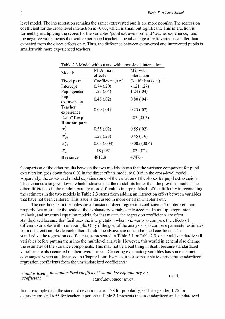
level model. The interpretation remains the same: extraverted pupils are more popular. The regression coefficient for the cross-level interaction is –0.03, which is small but significant. This interaction is formed by multiplying the scores for the variables ‘pupil extraversion’ and ‘teacher experience,’ and the negative value means that with experienced teachers, the advantage of extraverted is smaller than expected from the direct effects only. Thus, the difference between extraverted and introverted pupils is smaller with more experienced teachers.
Table 2.3 Model without and with cross-level interaction
Model: M1A: main effects
M2: with interaction
Fixed part Coefficient (s.e.) Coefficient (s.e.) Intercept 0.74 (.20) -1.21 (.27) Pupil gender 1.25 (.04) 1.24 (.04) Pupil extraversion 0.45 (.02) 0.80 (.04)
Teacher experience 0.09 (.01) 0.23 (.02)
Extra*T.exp -.03 (.003) Random part
2eσ 0.55 (.02) 0.55 (.02) 20uσ 1.28 (.28) 0.45 (.16)
22uσ 0.03 (.008) 0.005 (.004)
02uσ -.18 (.05) -.03 (.02) Deviance 4812.8 4747.6
Comparison of the other results between the two models shows that the variance component for pupil extraversion goes down from 0.03 in the direct effects model to 0.005 in the cross-level model. Apparently, the cross-level model explains some of the variation of the slopes for pupil extraversion. The deviance also goes down, which indicates that the model fits better than the previous model. The other differences in the random part are more difficult to interpret. Much of the difficulty in reconciling the estimates in the two models in Table 2.3 stems from adding an interaction effect between variables that have not been centered. This issue is discussed in more detail in Chapter Four. The coefficients in the tables are all unstandardized regression coefficients. To interpret them properly, we must take the scale of the explanatory variables into account. In multiple regression analysis, and structural equation models, for that matter, the regression coefficients are often standardized because that facilitates the interpretation when one wants to compare the effects of different variables within one sample. Only if the goal of the analysis is to compare parameter estimates from different samples to each other, should one always use unstandardized coefficients. To standardize the regression coefficients, as presented in Table 2.1 or Table 2.3, one could standardize all variables before putting them into the multilevel analysis. However, this would in general also change the estimates of the variance components. This may not be a bad thing in itself, because standardized variables are also centered on their overall mean. Centering explanatory variables has some distinct advantages, which are discussed in Chapter Four. Even so, it is also possible to derive the standardized regression coefficients from the unstandardized coefficients:
* . . .. . .
unstandardized coefficient stand dev explanatory varstandardizedcoefficient stand dev outcomevar
= (2.13)
In our example data, the standard deviations are: 1.38 for popularity, 0.51 for gender, 1.26 for extraversion, and 6.55 for teacher experience. Table 2.4 presents the unstandardized and standardized

Multilevel Analysis: Techniques and Applications 9
coefficients for the second model in Table 2.2. It also presents the estimates that we obtain if we first standardize all variables, and then carry out the analysis.
Table 2.4 Comparing unstandardized and standardized estimates
Model: Standardization using 2.13
Standardized variables
Fixed part Coefficient (s.e.) standardized
Coefficient (s.e.)
Intercept 0.74 (.20) - -.03 (.04) Pupil gender 1.25 (.04) 0.46 0.45 (.01) Pupil extraversion 0.45 (.02) 0.41 0.41 (.02)
Teacher experience 0.09 (.01) 0.43 0.43 (.04)
Random part 2eσ 0.55 (.02) 0.28 (.01) 20uσ 1.28 (.28) 0.15 (.02)
22uσ 0.03 (.008) 0.03 (.01)
02uσ -.18 (.05) -.01 (.01) Deviance 4812.8 3517.2
Table 2.4 shows that the standardized regression coefficients are almost the same as the coefficients estimated for standardized variables. The small differences in Table 2.4 are simply due to rounding errors. However, if we use standardized variables in our analysis, we find very different variance components and a very different value for the deviance. This is not only the effect of scaling the variables differently, which becomes clear if we realize that the covariance between the slope for pupil extraversion and the intercept is significant for the unstandardized variables, but not significant for the standardized variables. This kind of difference in results is general. The fixed part of the multilevel regression model is invariant for linear transformations, just as the regression coefficients in the ordinary single-level regression model. This means that if we change the scale of our explanatory variables, the regression coefficients and the corresponding standard errors change by the same multiplication factor, and all associated p-values remain exactly the same. However, the random part of the multilevel regression model is not invariant for linear transformations. The estimates of the variance components in the random part can and do change, sometimes dramatically. This is discussed in more detail in section 4.2 in Chapter Four. The conclusion to be drawn here is that, if we have a complicated random part, including random components for regression slopes, we should think carefully about the scale of our explanatory variables. If our only goal is to present standardized coefficients in addition to the unstandardized coefficients, applying equation 2.13 is safer than transforming our variables. On the other hand, we may estimate the unstandardized results, including the random part and the deviance, and then re-analyze the data using standardized variables, merely using this analysis as a computational trick to obtain the standardized regression coefficients without having to do hand calculations. 2.3 INSPECTING RESIDUALS Inspection of residuals is a standard tool in multiple regression analysis to examine whether assumptions of normality and linearity are met (cf. Stevens, 2009; Tabachnick & Fidell, 2007). Multilevel regression analysis also assumes normality and linearity. Since the multilevel regression model is more complicated than the ordinary regression model, checking such assumptions is even more important. For example, Bauer and Cai show that neglecting a non-linear relationship may result

Basic Two-Level Model
10
in spuriously high estimates of slope variances and cross-level interaction effects. Inspection of the residuals is one way to investigate linearity and homoscedasticity. There is one important difference from ordinary regression analysis; we have more than one residual, in fact, we have residuals for each random effect in the model. Consequently, many different residuals plots can be made. 2.3.1 Examples of Residuals Plots The equation below represents the one-equation version of the direct effects model for our example data. This is the multilevel model without the cross-level interaction. Since the interaction explains part of the extraversion slope variance, a model that does not include this interaction produces a graph that displays the actual slope variation more fully.
popularityij = γ00 + γ10 genderij + γ20 extraversionij + γ01 experiencej + u2j extraversionij + u0j + eij
In this model, we have three residual error terms: eij, u0j, and u2j. The eij are the residual prediction errors at the lowest level, similar to the prediction errors in ordinary single-level multiple regression. A simple boxplot of these residuals will enable us to identify extreme outliers. An assumption that is usually made in multilevel regression analysis is that the variance of the residual errors is the same in all groups. This can be assessed by computing a one-way analysis of variance of the groups on the absolute values of the residuals, which is the equivalent of Levene’s test for equality of variances in Analysis of Variance (Stevens, 1996). Raudenbush and Bryk (2002) describe a chi-square test that can be used for the same purpose. The u0j are the residual prediction errors at the group level, which can be used in ways analogous to the investigation of the lowest level residuals eij. The u2j are the residuals of the regression slopes across the groups. By plotting the regression slopes for the various groups, we get a visual impression of how much the regression slopes actually differ, and we may also be able to identify groups which have a regression slope that is wildly different from the others. To test the normality assumption, we can plot standardized residuals against their normal scores. If the residuals have a normal distribution, the plot should show a straight diagonal line. Figure 2.1 is a scatterplot of the standardized level-1 residuals, calculated for the final model including cross-level interaction, against their normal scores. The graph indicates close conformity to normality, and no extreme outliers. Similar plots can be made for the level-2 residuals.
Figure 2.1. Plot of level 1 standardized residuals against normal scores

Multilevel Analysis: Techniques and Applications 11
We obtain a different plot, if we plot the residuals against the predicted values of the outcome variable popularity, using the fixed part of the multilevel regression model for the prediction. Such a scatter plot of the residuals against the predicted values provides information about possible failure of normality, nonlinearity, and heteroscedasticity. If these assumptions are met, the plotted points should be evenly divided above and below their mean value of zero, with no strong structure (cf. Tabachnick & Fidell, 2007, p. 162). Figure 2.2 shows this scatter plot for the level-1 residuals. For our example data, the scatter plot in Figure 2.2 does not indicate strong violations of the assumptions.
Similar scatter plots can be made for the second level residuals for the intercept and the slope of the explanatory variable pupil extraversion. As an illustration, Figure 2.3 shows the scatterplots of the level-2 residuals around the average intercept and around the average slope of pupil extraversion against the predicted values of the outcome variable popularity. Both scatterplots indicate that the assumptions are reasonably met.
Figure 2.2. Level 1 standardized residuals plotted against predicted popularity
Figure 2.3. Level 2 residuals plotted against predicted popularity

Basic Two-Level Model
12
An interesting plot that can be made using the level-2 residuals, is a plot of the residuals against their rank order, with an added error bar. In Figure 2.4, an error bar frames each point estimate, and the classes are sorted in rank order of the residuals. The error bars represent the confidence interval around each estimate, constructed by multiplying its standard error by 1.39 instead of the more usual 1.96. Using 1.39 as multiplication factor results in confidence intervals with the property that if the error bars of two classes do not overlap, they have significantly different residuals at the 5% level (Goldstein, 2003). For a discussion of the construction and use of these error bars see Goldstein and Healy (1995) and Goldstein and Spiegelhalter (1996). In our example, this plot, sometimes called the caterpillar plot, shows some outliers at each end. This an indication of exceptional residuals for the intercept. A logical next step would be to identify the classes at the extremes of the rank order, and to seek for a post hoc interpretation of what makes these classes different.
Figure 2.4. Error bar plot of level 2 residuals
Examining residuals in multivariate models presents us with a problem. For instance, the residuals should show a nice normal distribution, which implies absence of extreme outliers. However, this applies to the residuals after including all important explanatory variables and relevant parameters in the model. If we analyze a sequence of models, we have a series of different residuals for each model, and scrutinizing them all at each step is not always practical. On the other hand, our decision to include a specific variable or parameter in our model might well be influenced by a violation of some assumption. Although there is no perfect solution to this dilemma, a reasonable approach is to examine the two residual terms in the intercept-only model, to find out if there are gross violations of the assumptions of the model. If there are, we should accommodate them, for instance by applying a normalizing transformation, by deleting certain individuals or groups from our data set, or by including a dummy variable that indicates a specific outlying individual or group. When we have determined our final model, we should make a more thorough examination of the various residuals. If we detect gross violations of assumptions, these should again be accommodated, and the model should be estimated again. Of course, after accommodating an extreme outlier, we might find that a previously significant effect has disappeared, and that we need to change our model again. Procedures for model exploration and detection of violations in ordinary multiple regression are discussed, for instance, in Tabachnick and Fidell (2007) or Field (2009). In multilevel regression, the same procedures apply, but the analyses are more complicated because we have to examine more than one set of residuals, and must distinguish between multiple levels. As mentioned in the beginning of this section, graphs can be useful in detecting outliers and

Multilevel Analysis: Techniques and Applications 13
nonlinear relations. However, an observation may have an undue effect on the outcome of a regression analysis without being an obvious outlier. Figure 2.5, a scatter plot of the so-called Anscombe data (Anscombe, 1973), illustrates this point. There is one data point in Figure 2.5, which by itself almost totally determines the regression line. Without this one observation, the regression line would be very different. Yet, when the residuals are inspected, it does not show up as an obvious outlier.
141210864
20
18
16
14
12
10
8
6
Figure 2.5. Regression line determined by one single observation
In ordinary regression analysis, various measures have been proposed to indicate the influence of individual observations on the outcome (cf. Tabachnick & Fidell, 2007). In general, such influence or leverage measures are based on a comparison of the estimates when a specific observation is included in the data or not. Langford and Lewis (1998) discuss extensions of these influence measures for the multilevel regression model. Since most of these measures are based on comparison of estimates with and without a specific observation, it is difficult to calculate them by hand. However, if the software offers the option to calculate influence measures, it is advisable to do so. If a unit (individual or group) has a large value for the influence measure, that specific unit has a large influence on the values of the regression coefficients. It is useful to inspect cases with extreme influence values for possible violations of assumptions, or even data errors. 2.3.2 Examining Slope Variation: OLS and Shrinkage Estimators The residuals can be added to the average values of the intercept and slope, to produce predictions of the intercepts and slopes in different groups. These can also be plotted.

Basic Two-Level Model
14
Figure 2.6. Plot of the 100 class regression slopes for pupil extraversion
For example, Figure 2.6 plots the 100 regression slopes for the explanatory variable pupil extraversion in the 100 classes. It is clear that for most classes the effect is strongly positive: extravert pupils tend to be more popular in all classes. It is also clear that in some classes the relationship is more pronounced than in other classes. Most of the regression slopes are not very different from the others, although there are a few slopes that are clearly different from the others. It could be useful to examine the data for these classes in more detail, to find out if there is a reason for the unusual slopes. The predicted intercepts and slopes for the 100 classes are not identical to the values we would obtain, if we carry out 100 separate ordinary regression analyses in each of the 100 classes, using standard Ordinary Least Squares (OLS) techniques. If we would compare the results from 100 separate OLS regression analyses to the values obtained from a multilevel regression analysis, we would find that the results from the separate analyses are more variable. This is because the multilevel estimates of the regression coefficients of the 100 classes are weighted. They are so-called Empirical Bayes (EB) or shrinkage estimates; a weighted average of the specific OLS estimate in each class and the overall regression coefficient, estimated for all similar classes. As a result, the regression coefficients are shrunk back towards the mean coefficient for the whole data set. The shrinkage weight depends on the reliability of the estimated coefficient. Coefficients that are estimated with small accuracy shrink more than very accurately estimated coefficients. Accuracy of estimation depends on two factors: the group sample size, and the distance between the group-based estimate and the overall estimate. Estimates in small groups are less reliable, and shrink more than estimates from large groups. Other things being equal, estimates that are very far from the overall estimate are assumed less reliable, and they shrink more than estimates that are close to the overall average. The statistical method used is called Empirical Bayes (EB) estimation. Due to this shrinkage effect, empirical Bayes estimators are biased. However, they are usually more precise, a property that is often more useful than being unbiased (cf. Kendall, 1959). The equation to form the empirical Bayes estimate of the intercepts is given by ( )EB OLS
0 0 00ˆ ˆ 1j j j jβ λ β λ γ= + − , (2.14)
where λj is the reliability of the OLS estimate OLS
0jβ as an estimate of βoj, which is given by the
equation ( )0 0
2 2 2j u u e jnλ σ σ σ= + (Raudenbush & Bryk, 2002), and γ00 is the overall intercept. The
Multilevel Analysis: Techniques and Applications 15
reliability λj is close to 1.0 when the group sizes are large and/or the variability of the intercepts across groups is large. In these cases, the overall estimate γ00 is not a good indicator of each group’s intercept. If the group sizes are small and there is little variation across groups, the reliability λj is close to 0.0, and more weight is put on the overall estimate γ00. Equation 2.14 makes clear that, since the OLS estimates are unbiased, the empirical Bayes estimates EB
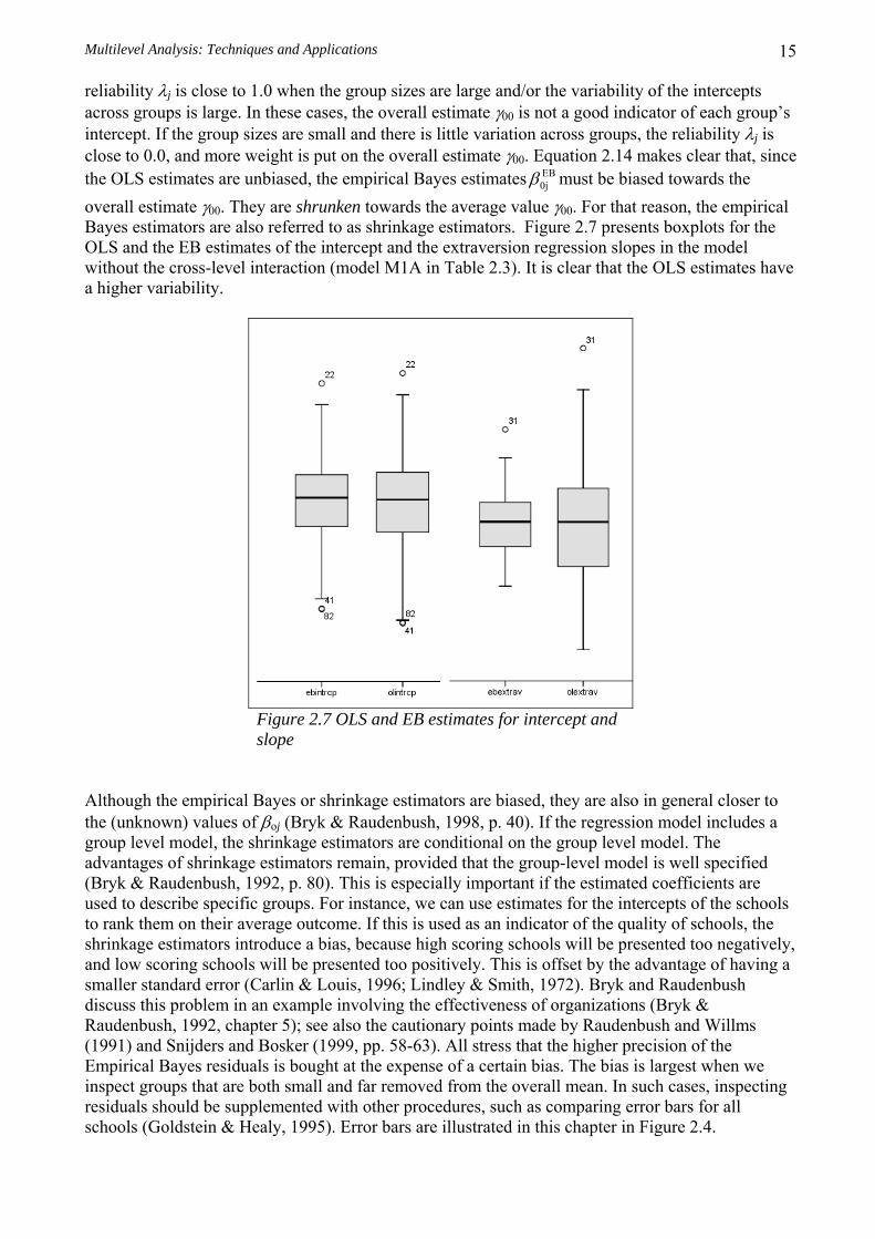
0jβ must be biased towards the overall estimate γ00. They are shrunken towards the average value γ00. For that reason, the empirical Bayes estimators are also referred to as shrinkage estimators. Figure 2.7 presents boxplots for the OLS and the EB estimates of the intercept and the extraversion regression slopes in the model without the cross-level interaction (model M1A in Table 2.3). It is clear that the OLS estimates have a higher variability.
Figure 2.7 OLS and EB estimates for intercept and slope
Although the empirical Bayes or shrinkage estimators are biased, they are also in general closer to the (unknown) values of βoj (Bryk & Raudenbush, 1998, p. 40). If the regression model includes a group level model, the shrinkage estimators are conditional on the group level model. The advantages of shrinkage estimators remain, provided that the group-level model is well specified (Bryk & Raudenbush, 1992, p. 80). This is especially important if the estimated coefficients are used to describe specific groups. For instance, we can use estimates for the intercepts of the schools to rank them on their average outcome. If this is used as an indicator of the quality of schools, the shrinkage estimators introduce a bias, because high scoring schools will be presented too negatively, and low scoring schools will be presented too positively. This is offset by the advantage of having a smaller standard error (Carlin & Louis, 1996; Lindley & Smith, 1972). Bryk and Raudenbush discuss this problem in an example involving the effectiveness of organizations (Bryk & Raudenbush, 1992, chapter 5); see also the cautionary points made by Raudenbush and Willms (1991) and Snijders and Bosker (1999, pp. 58-63). All stress that the higher precision of the Empirical Bayes residuals is bought at the expense of a certain bias. The bias is largest when we inspect groups that are both small and far removed from the overall mean. In such cases, inspecting residuals should be supplemented with other procedures, such as comparing error bars for all schools (Goldstein & Healy, 1995). Error bars are illustrated in this chapter in Figure 2.4.

Basic Two-Level Model
16
2.4 THREE- AND MORE-LEVEL REGRESSION MODELS 2.4.1 Multiple-level Models In principle, the extension of the two-level regression model to three and more levels is straightforward. There is an outcome variable at the first, the lowest level. In addition, there may be explanatory variables at all available levels. The problem is that three- and more-level models can become complicated very fast. In addition to the usual fixed regression coefficients, we must entertain the possibility that regression coefficients for first-level explanatory variables may vary across units of both the second and the third level. Regression coefficients for second-level explanatory variables may vary across units of the third level. To explain such variation, we must include cross-level interactions in the model. Regression slopes for the cross-level interaction between first-level and second-level variables may themselves vary across third-level units. To explain such variation, we need a three-way interaction involving variables at all three levels. The equations for such models are complicated, especially when we do not use the more compact summation notation but write out the complete single equation-version of the model in an algebraic format (for a note on notation see section 2.5). The resulting models are not only difficult to follow from a conceptual point of view; they may also be difficult to estimate in practice. The number of estimated parameters is considerable, and at the same time the highest level sample size tends to become relatively smaller. As DiPrete and Forristal (1994, p. 349) put it, the imagination of the researchers “…can easily outrun the capacity of the data, the computer, and current optimization techniques to provide robust estimates.” Nevertheless, three- and more-level models have their place in multilevel analysis. Intuitively, three-level structures such as pupils in classes in schools, or respondents nested within households, nested within regions, appear to be both conceptually and empirically manageable. If the lowest level is repeated measures over time, having repeated measures on pupils nested within schools again does not appear to be overly complicated. In such cases, the solution for the conceptual and statistical problems mentioned is to keep models reasonably small. Especially specification of the higher-level variances and covariances should be driven by theoretical considerations. A higher-level variance for a specific regression coefficient implies that this regression coefficient is assumed to vary across units at that level. A higher-level covariance between two specific regression coefficients implies that these regression coefficients are assumed to covary across units at that level. Especially when models become large and complicated, it is advisable to avoid higher-order interactions, and to include in the random part only those elements for which there is strong theoretical or empirical justification. This implies that an exhaustive search for second-order and higher-order interactions is not a good idea. In general, we should seek for higher-order interactions only if there is strong theoretical justification for their importance, or if an unusually large variance component for a regression slope calls for explanation. For the random part of the model, there are usually more convincing theoretical reasons for the higher-level variance components than for the covariance components. Especially if the covariances are small and insignificant, analysts sometimes do not include all possible covariances in the model. This is defensible, with some exceptions. First, it is recommended that the covariances between the intercept and the random slopes are always included. Second, it is recommended to include covariances corresponding to slopes of dummy-variables belonging to the same categorical variable, and for variables that are involved in an interaction or belong to the same polynomial expression (Longford, 1990, p. 79-80). 2.4.2 Intraclass Correlations in Three-Level Models In a two-level model, the intraclass correlation is calculated in the intercept-only model using equation 2.9, which is repeated below:

Multilevel Analysis: Techniques and Applications 17
0
0
2
2 2u
u e
σρ
σ σ=
+. (2.9, repeated)
The intraclass correlation is an indication of the proportion of variance at the second level, and it can also be interpreted as the expected (population) correlation between two randomly chosen individuals within the same group. If we have a three-level model, for instance pupils nested within classes, nested within schools, there are several ways to calculate the intraclass correlation. First, we estimate an intercept-only model for the three-level data, for which the single-equation model can be written as follows: Yijk = γ000 + v0k + u0jk + eijk . (2.15) The variances at the first, second, and third level are respectively 2
eσ , 0
2uσ , and
0
2vσ . The first method
(cf. Davis & Scott, 1995) defines the intraclass correlations at the class and school level as
0
0 0
2
2 2 2u
classv u e
σρ
σ σ σ=
+ +, (2.16)
and
0
0 0
2
2 2 2v
schoolv u e
σρ
σ σ σ=
+ +. (2.17)
The second method (cf. Siddiqui, Hedeker, Flay & Hu, 1996) defines the intraclass correlations at the class and school level as
0 0
0 0
2 2
2 2 2v u
classv u e
σ σρ
σ σ σ+
=+ +
, (2.18)
and
0
0 0
2
2 2 2v
schoolv u e
σρ
σ σ σ=
+ + . (2.19)
Actually, both methods are correct (Algina, 2000). The first method identifies the proportion of variance at the class and school level. This should be used if we are interested in a decomposition of the variance across the available levels, or if we are interested in how much variance is explained at each level (a topic discussed in section 4.5). The second method represents an estimate of the expected (population) correlation between two randomly chosen elements in the same group. So ρclass as calculated in equation 2.18 is the expected correlation between two pupils within the same class, and it correctly takes into account that two pupils who are in the same class must by definition also be in the same school. For this reason, the variance components for classes and schools must both be in the numerator of equation 2.18. If the two sets of estimates are different, which may happen if the amount of variance at the school level is large, there is no contradiction involved. Both sets of equations express two different aspects of the data, which happen to coincide when there are only two levels. 2.4.3. An Example of a Three-Level Model The data in this example are from a hypothetical study on stress in hospitals. The data are from nurses working in wards nested within hospitals. In each of 25 hospitals, four wards are selected and randomly assigned to an experimental and control condition. In the experimental condition, a
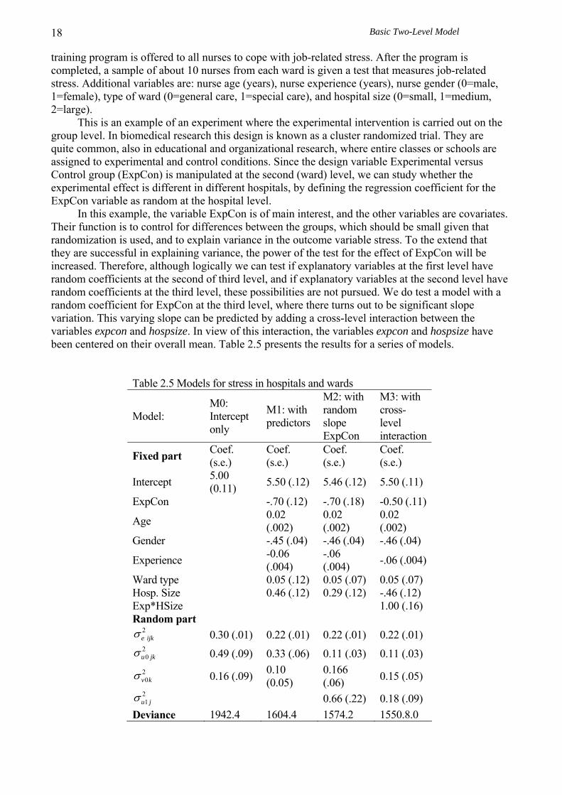
Basic Two-Level Model
18
training program is offered to all nurses to cope with job-related stress. After the program is completed, a sample of about 10 nurses from each ward is given a test that measures job-related stress. Additional variables are: nurse age (years), nurse experience (years), nurse gender (0=male, 1=female), type of ward (0=general care, 1=special care), and hospital size (0=small, 1=medium, 2=large). This is an example of an experiment where the experimental intervention is carried out on the group level. In biomedical research this design is known as a cluster randomized trial. They are quite common, also in educational and organizational research, where entire classes or schools are assigned to experimental and control conditions. Since the design variable Experimental versus Control group (ExpCon) is manipulated at the second (ward) level, we can study whether the experimental effect is different in different hospitals, by defining the regression coefficient for the ExpCon variable as random at the hospital level. In this example, the variable ExpCon is of main interest, and the other variables are covariates. Their function is to control for differences between the groups, which should be small given that randomization is used, and to explain variance in the outcome variable stress. To the extend that they are successful in explaining variance, the power of the test for the effect of ExpCon will be increased. Therefore, although logically we can test if explanatory variables at the first level have random coefficients at the second of third level, and if explanatory variables at the second level have random coefficients at the third level, these possibilities are not pursued. We do test a model with a random coefficient for ExpCon at the third level, where there turns out to be significant slope variation. This varying slope can be predicted by adding a cross-level interaction between the variables expcon and hospsize. In view of this interaction, the variables expcon and hospsize have been centered on their overall mean. Table 2.5 presents the results for a series of models.
Table 2.5 Models for stress in hospitals and wards
Model: M0: Intercept only
M1: with predictors
M2: with random slope ExpCon
M3: with cross-level interaction
Fixed part Coef. (s.e.)
Coef. (s.e.)
Coef. (s.e.)
Coef. (s.e.)
Intercept 5.00 (0.11) 5.50 (.12) 5.46 (.12) 5.50 (.11)
ExpCon -.70 (.12) -.70 (.18) -0.50 (.11)
Age 0.02 (.002)
0.02 (.002)
0.02 (.002)
Gender -.45 (.04) -.46 (.04) -.46 (.04)
Experience -0.06 (.004)
-.06 (.004) -.06 (.004)
Ward type 0.05 (.12) 0.05 (.07) 0.05 (.07) Hosp. Size 0.46 (.12) 0.29 (.12) -.46 (.12) Exp*HSize 1.00 (.16) Random part
2e ijkσ 0.30 (.01) 0.22 (.01) 0.22 (.01) 0.22 (.01) 20u jkσ 0.49 (.09) 0.33 (.06) 0.11 (.03) 0.11 (.03)
20v kσ 0.16 (.09) 0.10
(0.05) 0.166 (.06) 0.15 (.05)
21u jσ 0.66 (.22) 0.18 (.09)
Deviance 1942.4 1604.4 1574.2 1550.8.0

Multilevel Analysis: Techniques and Applications 19
The equation for the first model, the intercept-only model is
000 0 0ijk k jk ijkstress v u eγ= + + + . (2.20) This produces the variance estimates in the M0 column of Table 2.5. The proportion of variance (ICC) is 0.52 at the ward level, and 0.17 at the hospital level, calculated following equations 2.18 and 2.19. The nurse level and the ward level variances are evidently significant. The test statistic for the hospital level variance is Z=0.162/0.0852=1.901, which produces a one-sided p-value of 0.029. The hospital level variance is significant at the 5% level. The sequence of models in Table 2.5 shows that all predictor variables have a significant effect, except the ward type, and that the experimental intervention significantly lowers stress. The experimental effect varies across hospitals, and a large part of this variation can be explained by hospital size; in large hospitals the experimental effect is smaller. 2.5 A NOTE ABOUT NOTATION AND SOFTWARE 2.5.1 Notation In general, there will be more than one explanatory variable at the lowest level and more than one explanatory variable at the highest level. Assume that we have P explanatory variables X at the lowest level, indicated by the subscript p (p=1…P). Likewise, we have Q explanatory variables Z at the highest level, indicated by the subscript q (q=1…Q). Then, equation 2.5 becomes the more general equation: Yij = γ00 + γp0 Xpij + γ0q Zqj + γpq ZqjXpij + upj Xpij + u0j + eij . (2.20) Using summation notation, we can express the same equation as
00 0 0 0ij p pij q qj pq pij qj pj pij j ijp q p q p
Y X Z X Z u X u eγ γ γ γ= + + + + + +∑ ∑ ∑∑ ∑ . (2.21)
The errors at the lowest level eij are assumed to have a normal distribution with a mean of zero and a common variance σe² in all groups. The u-terms u0j and upj are the residual error terms at the highest level. They are assumed to be independent from the errors eij at the individual level, and to have a multivariate normal distribution with means of zero. The variance of the residual errors u0j is the variance of the intercepts between the groups, symbolized by
0
2uσ . The variances of the residual errors
upj are the variances of the slopes between the groups, symbolized by 2puσ . The covariances between
the residual error terms 'ppuσ are generally not assumed to be zero; they are collected in the higher level
variance/covariance matrix Ω.1 Note that in equation 2.15, γ00, the regression coefficient for the intercept, is not associated with an explanatory variable. We can expand the equation by providing an explanatory variable that is a constant equal to one for all observed units. This yields the equation Yij = γp0 Xpij + γpq ZqjXpij + upj Xpij + eij (2.22) where X0ij=1, and p=0…P. Equation 2.22 makes clear that the intercept is a regression coefficient, just like the other regression coefficients in the equation. Some multilevel software, for instance HLM
1 We may attach a subscript to Ω to indicate to which level it belongs. As long as there is no risk of confusion, the simpler notation without the subscript is used.

Basic Two-Level Model
20
(Raudenbush, Bryk, Cheongh & Congdon, 2004) puts the intercept variable X0=1 in the regression equation by default. Other multilevel software, for instance MLwiN (Rasbash, Steele, Browne & Prosser, 2005), requires that the analyst includes a variable in the data set that equals one in all cases, which must be added explicitly to the regression equation. In some cases, being able to eliminate the intercept term from the regression equation is a convenient feature. Equation 2.22 can be made very general if we let X be the matrix of all explanatory variables in the fixed part, symbolize the residual errors at all levels by u(l) with l denoting the level, and associate all error components with predictor variables Z, which may or may not be equal to the X. This produces the very general matrix formula Y=Xβ+Z(l)u(l) (cf. Goldstein, 1995, appendix 2.1). Since this book is more about applications than about mathematical statistics, it generally uses the algebraic notation, except when multivariate procedures such as structural equation modeling are discussed. The notation used in this book is close to the notation used by Goldstein (1987, 1995), Hox (1995), and Kreft and de Leeuw (1998). The most important difference is that these authors indicate the higher-level variance by σ00 instead of our
0
2uσ . The logic is that, if σ01 indicates the covariance between
variables 0 and 1, then σ00 is the covariance of variable 0 with itself, which is its variance. Bryk and Raudenbush (1992), and Snijders and Bosker (1999) use a different notation; they denote the lowest level error terms by rij, and the higher-level error terms by uj. The lowest level variance is σ2 in their notation. The higher-level variances and covariances are indicated by the Greek letter tau; for instance, the intercept variance is given by τ00. The τpp are collected in the matrix TAU, symbolized as Τ. The HLM program and manual in part use a different notation, for instance when discussing longitudinal and three-level models. In models with more than two levels, two different notational systems are used. One approach is to use different Greek characters for the regression coefficients at different levels, and different (Greek or Latin) characters for the variance terms at different levels. With many levels, this becomes cumbersome, and it is simpler to use the same character, say β for the regression slopes and u for the residual variance terms, and let the number of subscripts indicate to which level these belong. 2.5.2 Software Multilevel models can be formulated in two ways: (1) by presenting separate equations for each of the levels, and (2) by combining all equations by substitution into a single model-equation. The software HLM (Raudenbush et al., 2004) requires specification of the separate equations at each available level, but it can also show the single equation version. Most other software, e.g., MLwiN (Rasbash et al., 2005), SAS Proc Mixed (Littell et al., 1996)), SPSS command Mixed (Norusis, 2005) uses the single equation representation. Both representations have their advantages and disadvantages. The separate-equation representation has the advantage that it is always clear how the model is built up. The disadvantage is that it hides from view that modeling regression slopes by other variables results in adding an interaction to the model. As will be explained in Chapter Four, estimating and interpreting interactions correctly requires careful thinking. On the other hand, while the single-equation representation makes the existence of interactions obvious, it conceals the role of the complicated error components that are created by modeling varying slopes. In practice, to keep track of the model, it is recommended to start by writing the separate equations for the separate levels, and to use substitution to arrive at the single-equation representation. To take a quote from Singer’s excellent introduction to using SAS Proc Mixed for multilevel modeling (Singer, 1998, p. 350): “Statistical software does not a statistician make. That said, without software, few statisticians and even fewer empirical researchers would fit the kinds of sophisticated models being promulgated today.” Indeed, software does not make a statistician, but the advent of powerful and user-friendly software for multilevel modeling has had a large impact in research fields as diverse as education, organizational research, demography, epidemiology, and medicine. This book focuses on the conceptual and statistical issues that arise in multilevel modeling of complex data structures. It assumes that researchers who apply these techniques have access to and familiarity with some software that can estimate these models. Software is mentioned in various places, especially when a technique is discussed that requires specific software features or is only available in a specific
Multilevel Analysis: Techniques and Applications 21
program. Since statistical software evolves rapidly, with new versions of the software coming out much faster than new editions of general handbooks such as this, I do not discuss software setups or output in detail. As a result, this book is more about the possibilities offered by the various techniques than about how these things can be done in a specific software package. The techniques are explained using analyses on small but realistic data sets, with examples of how the results could be presented and discussed. At the same time, if the analysis requires that the software used have some specific capacities, these are pointed out. This should enable interested readers to determine whether their software meets these requirements, and assist them in working out the software setups for their favorite package.
In addition to the relevant program manuals, several software programs have been discussed in introductory articles. Using SAS Proc Mixed for multilevel and longitudinal data is discussed by Singer (1998). Peugh and Enders (2005) discuss SPSS Mixed using Singer’s examples. Both Arnold (1992), and Heck and Thomas (2000) discuss multilevel modeling using HLM as the software tool. Sullivan, Dukes and Losina (1999) discuss HLM and SAS Proc Mixed. West, Welch and Gatecki (2007) present a series of multilevel analyses using SAS, SPSS, R, Stata and HLM. Finally, the multilevel modeling program at the University of Bristol maintains a multilevel homepage that contains a series of software reviews. The homepage for this book (on www.geocities.com/joophox) contains links to these and other multilevel resources. The data used in the various examples are described in the appendix, and are all available through the Internet.
1
5
Analyzing Longitudinal Data Longitudinal data, or repeated measures data, can be viewed as multilevel data with repeated measurements nested within individuals. In its simplest form, this leads to a two-level model, with the series of repeated measures at the lowest level, and the individual subjects at the highest level. Longitudinal measures can be taken at fixed or at varying occasions. Multilevel analysis for longitudinal data can handle both situations. Since multilevel modeling does not require balanced data, it is not a problem if the number of available measurements is not the same for all individuals. This is an important benefit if there is panel dropout, or other forms of missing measurements within individuals. Since longitudinal data collected at fixed occasions is the simplest situation, this chapter starts with fixed occasions, and discusses varying occasions later.
If the data are collected to analyze individual change over time, the constructs under study must be measured on a comparable scale at each occasion (cf. Plewis, 1985, 1996; Taris, 2000). When the time span is short, this does not pose complicated problems. For instance, Tate and Hokanson (1993) report on a longitudinal study where the scores of students on the Beck Depression scale were collected at three occasions during the academic year. In such an application, especially when a well-validated measurement instrument is used, we may assume that the research instrument remains constant for the duration of the study. On the other hand, in a study that examines improvements in reading skill in school children from ages 5-12, it is clear that we cannot use the same instrument to measure reading skill at such different age levels. Here, we must make sure that the different measurement instruments are calibrated, meaning that a specific score has the same psychometric meaning at all age levels, independent of the actual reading test that is used. The issues are the same as the issues in cross-cultural comparison (cf. Bechger, van Schooten, de Glopper, & Hox, 1998). Another requirement is that there is sufficient time between the measurements that memory effects are not a problem. In some applications, this may not be the case. For instance, if data are collected that are closely spaced in time, we may expect considerable correlation between measurements collected at occasions that are close together, partly because of memory effects. These effects should then be included in the model, which leads to models with correlated errors. Formulating multilevel models for such situations can be quite complex. Some multilevel software has built-in provisions for modeling correlated errors. These are discussed in the last part of this chapter.
The models discussed in this chapter are all models for data that have repeated measures on individuals over time. Within the framework of multilevel modeling, we can also analyze data where the repeated measures are on higher levels, e.g., data where we follow the same set of schools over a number of years, with of course in each year a different set of pupils. Models for such data are similar to the models discussed in this chapter. Such repeated cross-sectional data are discussed by DiPrete and Grusky (1990) and Raudenbush and Chan (1993). Multilevel analysis models for longitudinal data are discussed in detail by Hedeker and Gibbons (2006) and by Singer and Willet (2003). Latent curve analysis using structural equation modeling is discussed by Duncan, Duncan and Strycker (2006) and by Bollen and Curran (2006). The structural equation approach to latent curve analysis is treated in this book in Chapter Sixteen.
Longitudinal Data
2
Multilevel analysis of repeated measures is often applied to data from large-scale panel surveys. In addition, it can also be a valuable analysis tool in a variety of experimental designs. If we have a pretest-posttest design, the usual analysis is an analysis of covariance (ANCOVA) with the experimental and control groups as the factor and the pretest as the covariate. In the multilevel framework, we analyze the slopes of the change over time, using an experimental group/control group dummy variable to predict differences in the slopes. If we have just a pretest-posttest design this does not offer much more than the usual analysis of covariance. However, in the multilevel framework it makes sense to add more measurement occasions between the pretest and the posttest. Willett (1989) and Maxwell (1998) show that the power of the test for differences between the experimental and the control groups can be increased dramatically by adding only a few additional waves of data collection. There is also an advantage on ANCOVA if there is dropout, especially if this is not completely random. Multilevel analysis of repeated measures can include incomplete cases, which is a major advantage when incomplete data indeed occur. 5.1 FIXED AND VARYING OCCASIONS It is useful to distinguish between repeated measures that are collected at fixed or varying occasions. If the measurements are taken at fixed occasions, all individuals provide measurements at the same set of occasions, usually regularly spaced, such as once every year. When occasions are varying, we have a different set of measures taken at different points in time for different individuals. Such data occur, for instance, in growth studies, where physical or psychological characteristics are studied for a set of individuals at different moments in their development. The data collection could be at fixed moments in the year, but the individuals would have different ages at that moment. Alternatively, the original design is a fixed occasion design, but due to planning problems, the data collection does not take place at the intended moments. For a multilevel analysis of the resulting data, the difference between fixed and varying occasions is not very important. For fixed occasion designs, especially when the occasions are regularly spaced and when there are no missing data, repeated measures analysis of variance (ANOVA) is a viable alternative for multilevel analysis. A comparison of the ANOVA approach and multilevel analysis is given in section 5.2. Another possibility in such designs is latent curve analysis, also known as latent growth curve analysis. This is a structural equation model (cf. Singer & Willett 2003; Duncan, Duncan & Strycker, 2006) that models a repeated measures polynomial analysis of variance. Latent growth curve models are treated in Chapter Sixteen. Multilevel models for longitudinal data are discussed by, among others, Bryk and Raudenbush (1987, Raudenbush & Bryk, 2002) and Goldstein (1987, 1995); for introductory articles see Snijders (1996), Cnaan, Laird and Slasor (1997), and Hedeker and Gibbons (2006). 5.2 EXAMPLE WITH FIXED OCCASIONS The example data are a longitudinal data set from 200 college students. The students’ Grade Point Average (GPA) has been recorded for six successive semesters. At the same time, it was recorded whether the student held a job in that semester, and for how many hours. This is recorded in a variable ‘job’ (= hours worked). In this example, we also use the student level variables High school GPA and gender (0=male, 1=female), which of course remain constant for each student across the six measurement occasions.
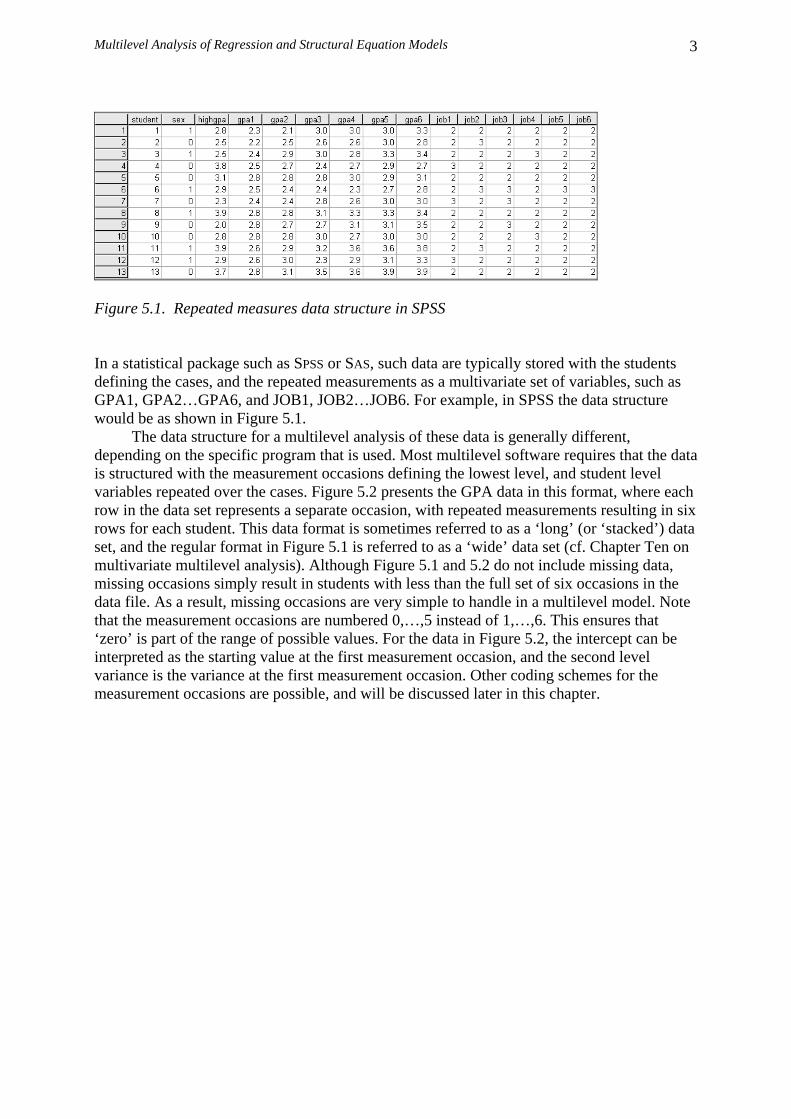
Multilevel Analysis of Regression and Structural Equation Models 3
Figure 5.1. Repeated measures data structure in SPSS In a statistical package such as SPSS or SAS, such data are typically stored with the students defining the cases, and the repeated measurements as a multivariate set of variables, such as GPA1, GPA2…GPA6, and JOB1, JOB2…JOB6. For example, in SPSS the data structure would be as shown in Figure 5.1. The data structure for a multilevel analysis of these data is generally different, depending on the specific program that is used. Most multilevel software requires that the data is structured with the measurement occasions defining the lowest level, and student level variables repeated over the cases. Figure 5.2 presents the GPA data in this format, where each row in the data set represents a separate occasion, with repeated measurements resulting in six rows for each student. This data format is sometimes referred to as a ‘long’ (or ‘stacked’) data set, and the regular format in Figure 5.1 is referred to as a ‘wide’ data set (cf. Chapter Ten on multivariate multilevel analysis). Although Figure 5.1 and 5.2 do not include missing data, missing occasions simply result in students with less than the full set of six occasions in the data file. As a result, missing occasions are very simple to handle in a multilevel model. Note that the measurement occasions are numbered 0,…,5 instead of 1,…,6. This ensures that ‘zero’ is part of the range of possible values. For the data in Figure 5.2, the intercept can be interpreted as the starting value at the first measurement occasion, and the second level variance is the variance at the first measurement occasion. Other coding schemes for the measurement occasions are possible, and will be discussed later in this chapter.

Longitudinal Data
4
Figure 5.2. Repeated measures data structure for multilevel analysis The multilevel regression model for longitudinal data is a straightforward application of the multilevel regression model described in Chapter Two. It can also be written as a sequence of models for each level. At the lowest, the repeated measures level, we have: 0 1 2ti i i ti i ti tiY T X eπ π π= + + + . (5.1) In repeated measures applications, the coefficients at the lowest level are often indicated by the Greek letter π. This has the advantage that the subject level coefficients, which in repeated measures are at the second level, can be represented by the usual Greek letter β, and so on. In equation (5.1), Yti is the response variable of individual i measured at measurement occasion t, T is the time variable that indicates the measurement occasion, and Xti is a time varying covariate. For example, Yti could be the GPA of a student at measurement occasion t, Tti indicates the occasion at which the GPA is measured, and Xti the job status of the student at time t. Student characteristics, such as gender, are time invariant covariates, which enter the equation at the second level:
0 00 01 0
1 10 11 1
2 20 21 2
i i i
i i i
i i i
Z uZ uZ u
π β βπ β βπ β β
= + +
= + +
= + +
(5.2)
By substitution, we get the single equation model:
00 10 20 01 11 21
1 2 0
ti ti ti i ti i ti i
i ti i ti i ti
Y T X Z T Z X Zu T u X u e
β β β β β β= + + + + +
+ + + +. (5.3)
Using variable labels instead of letters, the equation for our GPA example becomes:

Multilevel Analysis of Regression and Structural Equation Models 5
00 10 20 01
11 21
1 2 0
ti ti ti i
ti i ti i
i ti i ti i ti
Y Occasion Job SexOccasion Sex Job Sex
u Occasion u Job u e
β β β ββ β
= + + +
+ +
+ + + +
. (5.4)
In longitudinal research, we sometimes have repeated measurements of individuals, who are all measured together on a small number of fixed occasions. This is typically the case with experimental designs involving repeated measures and panel research. If we simply want to test the null hypothesis that the means are equal for all occasions, we can use repeated measures analysis of variance. If we use repeated measures univariate analysis of variance (Stevens, 2009, p. 420), we must assume sphericity. Sphericity means that there are complex restrictions on the variances and covariances between the repeated measures, for details see Stevens (2009, chapter 13). A specific form of sphericity, which is easily understood, is compound symmetry, sometimes referred to as uniformity. Compound symmetry requires that all population variances of the repeated measures are equal, and that all population covariances of the repeated measures are equal. If sphericity is not met, the F-ratio used in analysis of variance is positively biased, and we reject the null hypothesis too often. A different approach is to specify the repeated measures as observations on a multivariate response vector and use Multivariate Analysis of Variance (MANOVA). This does not require sphericity, and is considered the preferred approach if analysis of variance is used on repeated measures (O’Brien & Kaiser, 1985; Stevens, 2009). However, the multivariate test is more complicated, because it is based on a transformation of the repeated measures, and what is tested are actually contrasts among the repeated measures. A MANOVA analysis of the example data using the General Linear Model in SPSS (SPSS Inc., 1997) cannot easily incorporate a time-varying covariate such as job status. But MANOVA can be used to test the trend over time of the repeated GPA measures by specifying polynomial contrasts for the measurement occasions, and to test the fixed effects of gender and high school GPA. Gender is a dichotomous variable, which is entered as a factor, and high school GPA is a continuous variable that is entered as a covariate. Table 5.1 presents the results of the traditional significance tests.
Table 5.1 MANOVA significance tests on GPA example data Effect tested: F df P Occasion 3.58 5/193 .004 Occ. (linear) 8.93 1/197 .003 Occ.*HighGPA 0.87 5/193 .505 Occ.*Gender 1.42 5/193 .220 HighGPA 9.16 1/197 .003 Gender 18.37 1/197 .000
The MANOVA results indicate that there is a significant linear trend for the GPA measures. Both Gender and High school GPA have significant effects. The higher polynomial trends, which are not in the Table, are not significant, and the interactions between measurement occasion and High school GPA and gender are not significant. Table 5.2 presents the GPA means at the different measurement occasions, rounded to one decimal, for all six occasions, for male and female students.
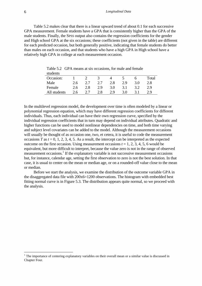
Longitudinal Data
6
Table 5.2 makes clear that there is a linear upward trend of about 0.1 for each successive GPA measurement. Female students have a GPA that is consistently higher than the GPA of the male students. Finally, the SPSS output also contains the regression coefficients for the gender and High school GPA at the six occasions; these coefficients (not given in the table) are different for each predicted occasion, but both generally positive, indicating that female students do better than males on each occasion, and that students who have a high GPA in High school have a relatively high GPA in college at each measurement occasion.
Table 5.2 GPA means at six occasions, for male and female students Occasion: 1 2 3 4 5 6 Total Male 2.6 2.7 2.7 2.8 2.9 3.0 2.8 Female 2.6 2.8 2.9 3.0 3.1 3.2 2.9 All students 2.6 2.7 2.8 2.9 3.0 3.1 2.9
In the multilevel regression model, the development over time is often modeled by a linear or polynomial regression equation, which may have different regression coefficients for different individuals. Thus, each individual can have their own regression curve, specified by the individual regression coefficients that in turn may depend on individual attributes. Quadratic and higher functions can be used to model nonlinear dependencies on time, and both time varying and subject level covariates can be added to the model. Although the measurement occasions will usually be thought of as occasion one, two, et cetera, it is useful to code the measurement occasions T as t = 0, 1, 2, 3, 4, 5. As a result, the intercept can be interpreted as the expected outcome on the first occasion. Using measurement occasions t = 1, 2, 3, 4, 5, 6 would be equivalent, but more difficult to interpret, because the value zero is not in the range of observed measurement occasions.1 If the explanatory variable is not successive measurement occasions but, for instance, calendar age, setting the first observation to zero is not the best solution. In that case, it is usual to center on the mean or median age, or on a rounded-off value close to the mean or median. Before we start the analysis, we examine the distribution of the outcome variable GPA in the disaggregated data file with 200x6=1200 observations. The histogram with embedded best fitting normal curve is in Figure 5.3. The distribution appears quite normal, so we proceed with the analysis.
1 The importance of centering explanatory variables on their overall mean or a similar value is discussed in Chapter Four.

Multilevel Analysis of Regression and Structural Equation Models 7
Figure 5.3. Histogram of GPA values in disaggregated data file Table 5.3 presents the results of a multilevel analysis of these longitudinal data. Model 1 is a model that contains only an intercept term and variances at the occasion and the subject level. The intercept of 2.87 in this model is simply the average GPA across all individuals and occasions. The intercept-only model estimates the repeated measures (level 1) variance as 0.098, and the subject level (level 2) variance as 0.057 (because these numbers are so small, they are given in 3 decimals). This estimates the total GPA variance as 0.155. Using equation 2.9, the intraclass correlation or the proportion variance at the subject level is estimated as ρ = 0.057/0.155 = 0.37. About one-third of the variance of the six GPA measures is variance between individuals, and about two-thirds is variance within individuals across time. In model 2, the Time variable is added as a linear predictor with the same coefficient for all subjects. The model predicts a value of 2.60 at the first occasion, which increases by 0.11 on each succeeding occasion. Just as in the MANOVA analysis, adding higher order polynomial trends for Time to the model does not improve prediction. Model 3 adds the time varying covariate Job status to the model. The effect of Job status is clearly significant; the more hours are worked, the lower the GPA. Model 4 adds the subject level (time invariant) predictors High school GPA and Sex. Both effects are significant; high school GPA correlates with average GPA in college, and female students perform better than male students.
Table 5.3 Results multilevel analysis of GPA, fixed effects
Model M1: Null model
M2: + occas.
M3: + job stat
M4: + high school GPA, gender
Fixed part Predictor coeff. (s.e.) coeff. (s.e.) coeff. (s.e.) coeff. (s.e.) Intercept 2.87 (.02) 2.60 (.02) 2.97 (.04) 2.64 (.10) Occasion 0.11 (.004) 0.10 (.003) 0.10 (.003)

Longitudinal Data
8
Job status -.17 (.02) -.17 (.02) GPA highschl 0.08 (.03) Gender 0.15 (.03) Random part
2eσ 0.098 (.004) 0.058 (.025) 0.055 (.002) 0.055 (.002) 20uσ 0.057 (.007) 0.063 (.007) 0.052 (.006) 0.045 (.01)
Deviance 913.5 393.6 308.4 282.8 AIC 919.5 401.6 318.4 296.8 BIC 934.7 422.0 343.8 332.4
In all models in Table 5.3, the Wald test indicates that the subject level (second level) variance is significant. The more accurate test using the difference of the deviance in a model with and a model without the second level variance term confirms this for all models in the table (results not reported here). If we compare the variance components of model 1 and model 2, we see that entering the measurement occasion variable decreases the occasion level variance considerably, while increasing the subject level variance by as much as 11%. If the usual formula is used to estimate the second level variance explained by the measurement occasion variable, we arrive at a negative value for the amount of explained variance. This is odd, but it is in fact typical for multilevel analysis of repeated measures. The occurrence of negative estimates for the explained variance makes it impossible to use the residual error variance of the intercept-only model as a benchmark, and to examine how much this goes down when explanatory variables are added to the model.
The reason for this apparent anomaly is, as is discussed in detail in Chapter Four, that the ‘amount of variance explained at a specific level’ is not a simple concept in multilevel models (cf. Snijders & Bosker, 1994). The problem arises because the statistical model behind multilevel models is a hierarchical sampling model: groups are sampled at the higher level, and at the lower level individuals are sampled within groups. This sampling process creates some variability in all variables between the groups, even if there are in fact no real group differences. In a time series design, the lowest level is a series of measurement occasions. In many cases, the data collection design is set up to make sure that the repeated measurements are evenly spaced and the data are collected at the same time for all individuals in the sample. Therefore, the variability between subjects in the measurement occasion variable is usually much higher than the hierarchical sampling model assumes. Consequently, the intercept-only model overestimates the variance at the occasion level, and underestimates the variance at the subject level. Model 2 uses the measurement occasion variable to model the occasion level variance in the dependent variable GPA. Conditional upon this effect, the variances estimated at the measurement occasions and at the subject level are much more realistic.
Chapter Four in this book describes procedures based on Snijders and Bosker (1994) to correct the problem. A simple approximation is to use as a baseline model for the ‘explained variance’ a model that includes the measurement occasion in an appropriate manner. Whether this is linear or needs to be some polynomial must be determined by preliminary analyses. In our example, a linear trend for measurement occasion suffices. Using M2 in Table 5.3 as the baseline, we calculate that job status explains (0.058-0.055)/0.058=0.052 or 5.2% of the variance, indicating that in semesters that they work more hours off campus, students tend to have a lower grade. The time-varying predictor job status explains a further (0.063-0.052/0.063)=0.175 or 17.5% of the variance between students; apparently students differ in how many hours they work in an off campus job. Hence, although job status is a time-varying

Multilevel Analysis of Regression and Structural Equation Models 9
predictor, it explains more variation between different subjects in the same semester, than within the same subjects from one semester to the next. The pupil level variables gender and High school GPA explain an additional 11.5% of the between students variance. The models presented in Table 5.3 all assume that the rate of change is the same for all individuals. In the models presented in Table 5.4, the regression coefficient of the measurement occasion variable is assumed to vary across individuals.
Table 5.4 Results multilevel analysis of GPA, varying effects for occasion
Model
M5: + occasion random
M6: + cross-level interaction standardized
Fixed part Predictor coeff. (s.e.) coeff. (s.e.) Intercept 2.56 (.10) 2.58 (.09) Occasion 0.10 (.006) 0.09 (.01) 0.38 Job status -.13 (.02) -.13 (.02) -.14 GPA highschl 0.09 (.03) 0.09 (.03) 0.13 Gender 0.12 (.03) 0.08 (.03) 0.10 Occas*Gender 0.03 (.01) 0.13 Random part
2eσ 0.042 (.002) 0.042 (.002) 20uσ 0.038 (.006) 0.038 (.01)
21uσ 0.004 (.001) 0.004 (.001)
01uσ -.002 (.002) -.002 (.001) ru01 -.21 -.19 Deviance 170.1 163.0 AIC 188.1 183.0 BIC 233.93 233.87
In model 5 in Table 5.4, the slope of the measurement occasion variable is allowed to vary across individuals. The Wald test for the variance of the slopes for occasion is significant, Z=6.02 (calculated carrying more decimal values than reported in Table 5.4). The deviance difference test (comparing model 5 to the same model without the subject level variance) produces a chi-square of 109.62. With one degree of freedom, this translates to Z=10.47, which demonstrates again that for variances the deviance difference test is generally more powerful than the Wald test. The variance components for the intercept and the regression slope for the time variable are both significant. The significant intercept variance of 0.038 means that individuals have different initial states, and the significant slope variance of 0.004 means that individuals also have different rates of change. In model 6, the interaction of the Occasion variable with the subject level predictor Gender is added to the model. The interaction is significant, but including it does not decrease the slope variance for the time variable (actually, carrying all decimals in the output leads to a decrease in slope variance of 0.00022). The variance component of 0.004 for the slopes of the occasion variable does not seem large. However, multilevel models assume a normal distribution for these slopes (or, equivalently, for the slope residuals u1), for which the standard deviation is estimated in model 5
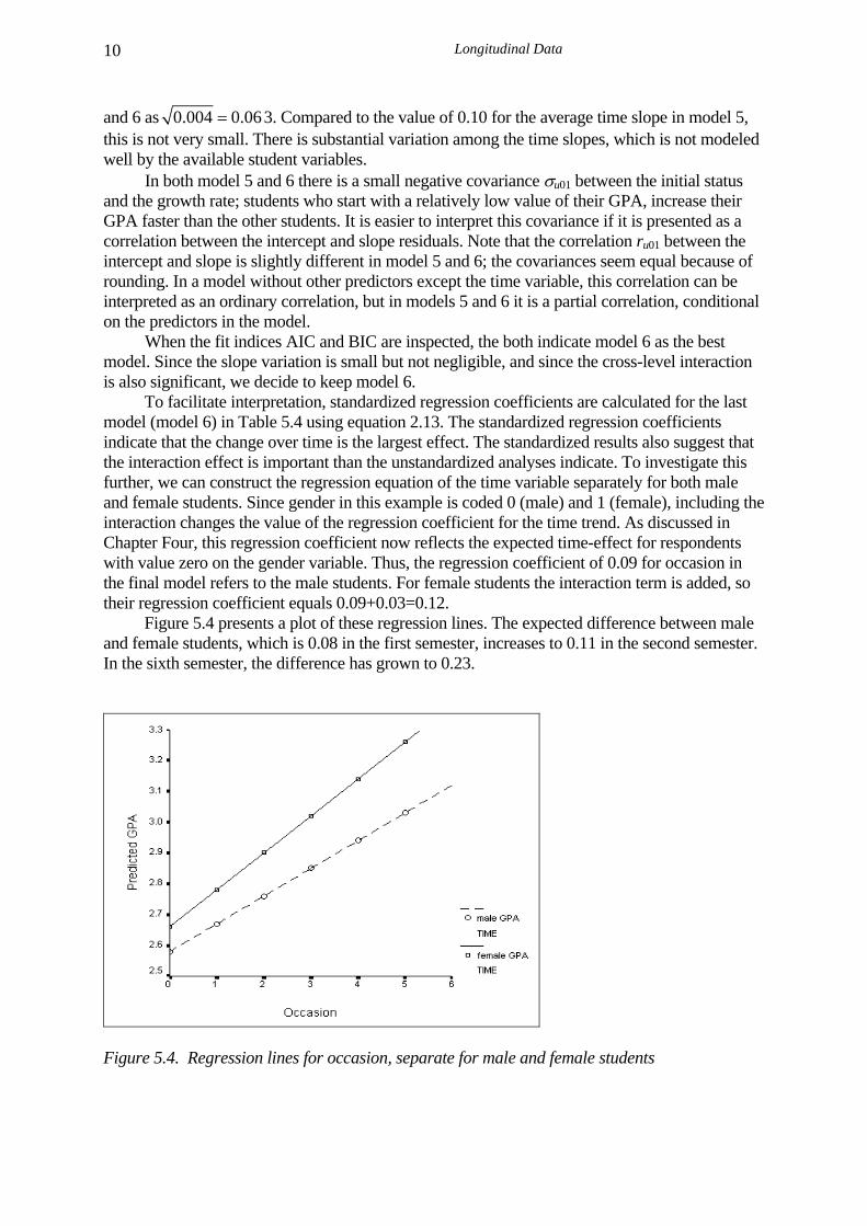
Longitudinal Data
10
and 6 as 0.004 0.06= 3. Compared to the value of 0.10 for the average time slope in model 5, this is not very small. There is substantial variation among the time slopes, which is not modeled well by the available student variables.
In both model 5 and 6 there is a small negative covariance σu01 between the initial status and the growth rate; students who start with a relatively low value of their GPA, increase their GPA faster than the other students. It is easier to interpret this covariance if it is presented as a correlation between the intercept and slope residuals. Note that the correlation ru01 between the intercept and slope is slightly different in model 5 and 6; the covariances seem equal because of rounding. In a model without other predictors except the time variable, this correlation can be interpreted as an ordinary correlation, but in models 5 and 6 it is a partial correlation, conditional on the predictors in the model.
When the fit indices AIC and BIC are inspected, the both indicate model 6 as the best model. Since the slope variation is small but not negligible, and since the cross-level interaction is also significant, we decide to keep model 6. To facilitate interpretation, standardized regression coefficients are calculated for the last model (model 6) in Table 5.4 using equation 2.13. The standardized regression coefficients indicate that the change over time is the largest effect. The standardized results also suggest that the interaction effect is important than the unstandardized analyses indicate. To investigate this further, we can construct the regression equation of the time variable separately for both male and female students. Since gender in this example is coded 0 (male) and 1 (female), including the interaction changes the value of the regression coefficient for the time trend. As discussed in Chapter Four, this regression coefficient now reflects the expected time-effect for respondents with value zero on the gender variable. Thus, the regression coefficient of 0.09 for occasion in the final model refers to the male students. For female students the interaction term is added, so their regression coefficient equals 0.09+0.03=0.12. Figure 5.4 presents a plot of these regression lines. The expected difference between male and female students, which is 0.08 in the first semester, increases to 0.11 in the second semester. In the sixth semester, the difference has grown to 0.23.
Figure 5.4. Regression lines for occasion, separate for male and female students

Multilevel Analysis of Regression and Structural Equation Models 11
Since the measurement occasion variable is coded in such a way that the first occasion is coded as zero, the negative correlation between the intercepts and slopes refers to the situation on the first measurement. As is explained in section 4.2 of Chapter Four, the estimates of the variance components in the random part can change if the scale of the time variable is changed. In many models, this is not a real problem, because the interest is mostly in estimation and interpretation of the regression coefficients in the fixed part of the model. In repeated measures analysis, the correlation between the intercepts and the slopes of the time variable is often an interesting parameter, to be interpreted along with the regression coefficients. In this case, it is important to realize that this correlation is not invariant; it changes if the scale of the time variable is changed. In fact, one can show that by using extremely different scalings for the time variable, we can give the correlation between the intercepts and slopes any desired value (Stoel & van den Wittenboer, 2001). Table 5.5 illustrates this point. Table 5.5 shows the effect of different scalings of the time variable on the coefficients of model 5. In model 5a, the time variable is scaled as in all our analyses so far, with the first measurement occasion coded as zero. In model 5b, the time variable is coded with the last measurement occasion coded as zero, and the earlier occasions with negative values –5, …, -1. In model 5c, the time variable is centered on its overall mean. From the correlations between the intercepts and slopes for the time-variable, we conclude in model 5b that students who end with a relatively high GPA, on average have a steeper GPA increase over time. In the centered model, 5c, this correlation is lower, but still quite clear. If we inspect the first model 5a, which codes the first occasion as zero, we see a negative correlation, meaning that subjects with a relatively low initial GPA have a steeper growth rate. It is clear that we cannot interpret the correlation between the intercept and slopes directly. This correlation can only be interpreted in combination with the scale on which the occasion variable is defined.1
Table 5.5 Results model 5 for different scalings of measurement occasion
Model
M5a: first occasion=0
M5b: last occasion=0
M5c: occasions centered
Fixed part Predictor coeff. (s.e.) coeff. (s.e.) Intercept 2.56 (.10) 3.07 (.09) 2.82 (.09) Occasion 0.10 (.006) 0.10 (.006) 0.10 (.006) Job status -.13 (.02) -.13 (.02) -.13 (.02) GPA highschl 0.09 (.03) 0.09 (.03) 0.09 (.03) Gender 0.12 (.03) 0.12 (.03) 0.12 (.03) Random part
2eσ 0.042 (.002) 0.042 (.002) 0.042 (.002) 20uσ 0.038 (.006) 0.109 (.014) 0.050 (.006)
21uσ 0.004 (.001) 0.004 (.001) 0.004 (.001)
01uσ -.002 (.002) 0.017 (.003) 0.007 (.001) ru01 -.21 0.82 0.51 Deviance 170.1 170.1 170.1
1 The point on the t scale where the correlation flips from negative to positive is t*=t0-(u01/u11)), where t0 is the current zero-point on the time axis. This is also the point where the intercept variance is the lowest (Mehta & West, 2000).
Longitudinal Data
12
AIC 188.1 188.1 188.1 BIC 233.9 233.9 233.9
Note that the three models in Table 5.5 have exactly identical estimates for all parameters that do not involve the measurement occasion, and exactly the same deviance and fit measures. The models are in fact equivalent. The different ways that the time variable is coded lead to what statisticians call a re-parameterization of the model. The three models all describe the data equally well, and are equally valid. Nevertheless, they are not identical. The situation is comparable to viewing a landscape from different angles. The landscape does not change, but some views are more interesting than others are. The important lesson here is that in repeated measures analysis, careful thought must be given to the coding of the time variable. As stated, by a judicious choice of scale, we can give the correlation between the intercept and slope residuals any value that we want. If the zero-point is far outside the observed values, for instance if we code the occasions as 2004, 2005, 2006, 2007, 2008 and 2009, which does make some sense, we will get an extreme correlation. If we want to interpret the correlation between the intercepts and slopes, we must make sure that the zero-point has a strong substantive meaning. Adding a graphical display of the slopes for different individuals may help to interpret the results.1 5.3 EXAMPLE WITH VARYING OCCASIONS The data in the next example are a study of children’s development in reading skill and antisocial behavior. The data are a sample of 405 children who were within the first two years of entry to elementary school. The data consist of four repeated measures of both the child’s antisocial behavior and the child’s reading recognition skills. In addition, at the first measurement occasion, measures were collected of emotional support and cognitive stimulation provided by the mother. Other variables are the child’s gender and age and the mother’s age at the first measurement occasion. The data were collected using face-to-face interviews of both the child and the mother at two-year intervals between 1986 and 1992. Between 1986 and 1992 there was an appreciable amount of panel dropout: all N=405 children and mothers were interviewed at measurement occasion 1, but on the three subsequent occasions the sample sizes were 374, 297 and 294. Only 221 cases were interviewed at all four occasions. This data sett was compiled by Curran (1997) from a large longitudinal data set. The predominant dropout pattern in this data set is panel dropout, meaning that if a subject was not measured at some measurement occasion, that subject is also not measured at subsequent measurement occasions. However, a small number of subjects were not measured at one of the measurement occasions, but did return at subsequent occasions.
1 In large data sets this display will be confusing, and it is better to present a plot of a random or selected subsample of the individuals.

Multilevel Analysis of Regression and Structural Equation Models 13
Figure 5.5 Child ages at the first measurement occasion These data are a good example of data with varying measurement occasions. Although the measurement occasions are the same for all children, their ages are all different. The children’s ages at the first measurement occasion vary from 6 to 8 years. The children’s ages were coded in months, and there are 25 different values for this variable. Since each child is measured at most four times, these 25 values are best treated as a time-varying predictor indicating varying measurement occasions. Figure 5.5 shows the frequency of different ages at the start of the data collection. It is clear that with 25 different ages and only four measurement occasions, using the real age in a MANOVA-type analysis is impossible, because using listwise deletion would leave no cases to analyze. Restructured in the ‘long’ or ‘stacked’ format, we have the children’s age varying from 6 to 14 years, and 1325 out of a possible 1620 observations for reading skill available for the analysis. Figure 5.6 shows a scatterplot for reading skill by child age, with the best fitting nonlinear fit line (the loess fit function) added. The relationship is mostly linear, reading skill increasing with age, but with some deceleration of the upwards trend at the higher ages. The variance of reading skills increases with age, which indicates that the regression coefficient for age is likely to vary across subjects.
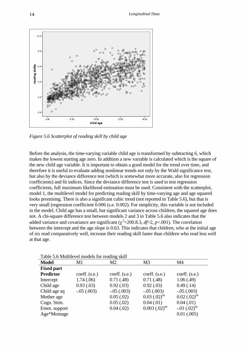
Longitudinal Data
14
Figure 5.6 Scatterplot of reading skill by child age Before the analysis, the time-varying variable child age is transformed by subtracting 6, which makes the lowest starting age zero. In addition a new variable is calculated which is the square of the new child age variable. It is important to obtain a good model for the trend over time, and therefore it is useful to evaluate adding nonlinear trends not only by the Wald significance test, but also by the deviance difference test (which is somewhat more accurate, also for regression coefficients) and fit indices. Since the deviance difference test is used to test regression coefficients, full maximum likelihood estimation must be used. Consistent with the scatterplot, model 1, the multilevel model for predicting reading skill by time-varying age and age squared looks promising. There is also a significant cubic trend (not reported in Table 5.6), but that is very small (regression coefficient 0.006 (s.e. 0.002). For simplicity, this variable is not included in the model. Child age has a small, but significant variance across children, the squared age does not. A chi-square difference test between models 2 and 3 in Table 5.6 also indicates that the added variance and covariance are significant (χ2=200.8.3, df=2, p<.001). The correlation between the intercept and the age slope is 0.63. This indicates that children, who at the initial age of six read comparatively well, increase their reading skill faster than children who read less well at that age.
Table 5.6 Multilevel models for reading skill Model M1 M2 M3 M4 Fixed part Predictor coeff. (s.e.) coeff. (s.e.) coeff. (s.e.) coeff. (s.e.) Intercept 1.74 (.06) 0.71 (.48) 0.71 (.48) 1.06 (.49) Child age 0.93 (.03) 0.92 (.03) 0.92 (.03) 0.49 (.14) Child age sq -.05 (.003) -.05 (.003) -.05 (.003) -.05 (.003) Mother age 0.05 (.02) 0.03 (.02)ns 0.02 (.02)ns Cogn. Stim. 0.05 (.02) 0.04 (.01) 0.04 (.01) Emot. support 0.04 (.02) 0.003 (.02)ns -.01 (.02)ns Age*Momage 0.01 (.005)

Multilevel Analysis of Regression and Structural Equation Models 15
Age*Emot 0.01 (.004) Random part
2eσ 0.39 (.02) 0.39 (.02) 0.27 (.02) 0.28 (.02) 20uσ 0.66 (.06) 0.60 (.04) 0.21 (.04) 0.21 (.04)
21uσ 0.02 (.003) 0.01 (.003)
01uσ 0.04 (.001) 0.04 (.001) ru01 0.64 Deviance 3245.0 3216.2 3015.4 2995.3 AIC 3255.0 3232.2 3035.4 3019.3 BIC 3281.0 3273.7 3087.3 3081.6
The time invariant variables mother age, cognitive stimulation, and emotional support, which were measured at the first measurement occasion, have significant effects in the fixed model, but two of these become nonsignificant when the effect of age is assumed to vary across the children, then only cognitive stimulation has a significant regression coefficient. The deviance difference between models M2 and M3 is 200.8. As explained in Chapter Three, given that we test both an unconstrained covariance and a variance that is constrained to be non-negative, the appropriate test is a mixture of 50% chi-square with one degree of freedom and 50% chi-square with two degrees of freedom. Given the large value of χ2=200.8, a test at the conservative df=2 produces a very small p-value p<0.001. The decreasing AIC and BIC also suggest that model 3 is preferable. Thus, the varying effect of age belongs in the model, and the significant effect of mother age and emotional support in the Fixed model are spurious. To model the significant variance of the regression coefficient of child age, cross-level interactions of child age with the three time invariant variables are added to the model. In this model, the interactions between the child’s age and mother age and between the child’s age and emotional support were significant. As a consequence, the direct effects of mother age and emotional support are retained in the model, although these direct effects are not significant by themselves. The interaction between child age and cognitive stimulation is not significant, and is dropped from the model. The last column of Table 5.6 presents the estimates for this final model. Both the deviance difference test (χ2=20.1, df=2, p<.001) and the decrease in AIC and BIC indicate that model 4 is better than model 3. However, the variance of the coefficients for child age is the same in two decimal places; when more decimals are carried it turns out that the two interaction effects explain only 0.9% of the slope variance. The coefficients for the interactions are both 0.01. This means that when the mother age is higher, or the emotional support is high, the reading skill increases faster with the child’s age. Plots are useful to interpret such interactions, Figure 5.7 shows the estimated fit lines for mothers of different ages (the range in the data is 21-29) and low vs. high emotional support (the range in the data is 0-13). Figure 5.7 illustrates that for older mothers the increase in reading skill is steeper and the leveling off less sharp. The same holds for high emotional support, with high emotional support the increase in reading skill is steeper and the leveling off less sharp. Note that the curves in Figure 5.7 are the predicted outcomes disregarding all variables not involved in the cross-level interaction. It shows the theoretical effect of the interaction, not the trend in the actual data. The apparent downward trend at the higher ages is the result of extrapolating the quadratic trend.

Longitudinal Data
16
Figure 5.7 Estimated fit lines for reading by mothers of different ages and low vs. high emotional support
5.4 ADVANTAGES OF MULTILEVEL ANALYSIS FOR LONGITUDINAL DATA Using multilevel models to analyze repeated measures data has several advantages. Bryk and Raudenbush (1992) mention five key points. First, by modeling varying regression coefficients at the measurement occasion level, we have growth curves that are different for each subject. This fits in with the way individual development is generally conceptualized (cf. Willett, 1988). Second, the number of repeated measures and their spacing may differ across subjects. Other analysis methods for longitudinal data cannot handle such data well. Third, the covariances between the repeated measures can be modeled as well, by specifying a specific structure for the variances and covariances at either level. This approach will be discussed in section 5.5. Fourth, if we have balanced data and use RML estimation, the usual analysis of variance based F-tests and t-tests can be derived from the multilevel regression results (cf. Raudenbush, 1993a). This shows that analysis of variance on repeated measures is a special case of the more general multilevel regression model. Fifth, in the multilevel model it is simple to add higher levels, to investigate the effect of family or social groups on individual development. A sixth advantage, not mentioned by Bryk and Raudenbush, is that it is straightforward to include time varying or time constant explanatory variables to the model, which allows us to model both the average group development and the development of different individuals over time. 5.5 COMPLEX COVARIANCE STRUCTURES If multilevel modeling is used to analyze longitudinal data, the variances and covariances between different occasions have a very specific structure. In a two-level model with only a random intercept at both levels, the variance at any measurement occasion has the value
0
2 2e uσ σ+ , and the covariance between any two measurement occasions has the value
0
2uσ . Thus,
for the GPA example data, a simple linear trend model as specified by equation (5.1) is
Multilevel Analysis of Regression and Structural Equation Models 17
GPAti = β00 + β10Occasionti + u0i + eti , (5.5) where the residual variance on the occasion level is given by 2
eσ , and the residual error on the subject level is given by
0
2uσ . For this and similar models without additional random effects, the
matrix of variances and covariances among the occasions is given by (Goldstein, 1995; Raudenbush & Bryk, 2002):
( )
0 0 0 0
0 0 0 0
0 0 0 0
0 0 0 0
2 2 2 2 2
2 2 2 2 2
2 2 2 2 2
2 2 2 2 2
Y
e u u u u
u e u u u
u u e u u
u u u e u
σ σ σ σ σ
σ σ σ σ σ
σ σ σ σ σ
σ σ σ σ σ
⎛ ⎞+ …⎜ ⎟
+ …⎜ ⎟⎜ ⎟+ …Σ = ⎜ ⎟⎜ ⎟⎜ ⎟⎜ ⎟… +⎝ ⎠
. (5.6)
In the covariance matrix (5.6), all variances are equal, and all covariances are equal. This shows that the standard multilevel model, with a single error term at the occasion and at the subject level, is the same as assuming compound symmetry, the same restrictive assumption that is made in univariate analysis of variance for repeated measures. According to Stevens (2009), if the assumption of compound symmetry is violated, the standard ANOVA significance tests are too lenient, and reject the null hypothesis more often than is warranted. Therefore, MANOVA is preferred, which estimates all variances and covariances among occasions without restrictions. Bryk and Raudenbush (1992, p. 132) argue that uncorrelated errors may be appropriate in short time series. However, the assumption of uncorrelated errors is not essential, because the multilevel regression model can easily be extended to include an unconstrained covariance matrix at the lowest level (Goldstein, 2003). To model correlated errors, we use a multivariate response model (treated in more detail in Chapter Ten in this book) with a full set of dummy variables indicating the six consecutive measurement occasions. Thus, if we have p measurement occasions, we have p dummy variables, one for each occasion. The intercept term is removed from the model, so the lowest level is empty. The dummy variables are all allowed to have random slopes at the second level. Thus, for our grade point example with six occasions, we have six dummy variables O1, O2, …, O6, and the equation for a model without additional explanatory variables becomes: GPAti = β10O1i + β20O2i + β30O3i + β40O4i + β50O5i + β60O6i + u10iO1i + u20iO2i + u30iO3i + u40iO4i + u50iO5i + u60iO6i . (5.7) Having six random slopes at level two provides us with a 6×6 covariance matrix for the six occasions. This is often denoted as an unstructured model for residual errors across time; all possible variances and covariances are estimated. The unstructured model for the random part is also a saturated model; all possible parameters are estimated and it cannot fail to fit. The regression slopes β10 to β60 are simply the estimated means at the six occasions. Equation 5.7 defines a multilevel model that is equivalent to the MANOVA approach. Maas and Snijders (2003) discuss model 5.7 at length, and show how the familiar F-ratio’s from the MANOVA approach can be calculated from the multilevel software output. An attractive property of the multilevel approach here is that it is not affected by missing data. Delucchi and Bostrom (1999) compare the MANOVA and the multilevel approach to longitudinal data using small samples with missing data. Using simulation, they conclude that the multilevel approach is more accurate than the MANOVA approach.

Longitudinal Data
18
The model in equation 5.7 is equivalent to a MANOVA model. Since the covariances between the occasions are estimated without restrictions, it does not assume compound symmetry. However, the fixed part is also fully saturated; it estimates the six means at the six measurement occasions. To model a linear trend over time, we must replace the fixed part of equation 5.7 with the fixed part for the linear trend in equation 5.5. This gives us the following model: GPAti= β00 + β10Tti + u10iO1i + u20iO2i + u30iO3i + u40iO4i + u50iO5i + u60iO6i . (5.8) To specify model 5.8 in standard multilevel software we must specify an intercept term that has no second-level variance component and six dummy variables for the occasions that have no fixed coefficients. Some software has built-in facilities for modeling specific covariance structures over time. If there are no facilities for longitudinal modeling, model equation 5.8 requires that the regression coefficients for the occasion dummies are restricted to zero, while their slopes are still allowed to vary across individuals. At the same time, an intercept and a linear time trend is added, which may not vary across individuals. The covariance matrix between the residual errors for the six occasions has no restrictions. If we impose the restriction that all variances are equal, and that all covariances are equal, we have again the compound symmetry model. This shows that the simple linear trend model in 5.5 is one way to impose the compound symmetry structure on the random part of the model. Since model 5.5 is nested in model 5.7, we can use the overall chi-square test based on the deviance of the two models to test if the assumption of compound symmetry is tenable. Models with a residual error structure over time as in model 5.6 are very complex, because they assume a saturated model for the error structure. If there are k measurement occasions, the number of elements in the covariance matrix for the occasions is k(k+1)/2. So, with six occasions, we have 21 elements to be estimated. If the assumption of compound symmetry is tenable, models based on this model (cf. equation 5.5) are preferable, because they are more compact. Their random part requires only two elements ( 2
eσ and 0
2uσ .) to be estimated. The
advantage is not only that smaller models are more parsimonious, but they are also easier to estimate. However, the compound symmetry model is very restrictive, because it assumes that there is one single value for all correlations between measurement occasions. This assumption is in many cases not very realistic, because the error term contains all omitted sources of variation (including measurement errors), which may be correlated over time. Different assumptions about the autocorrelation over time lead to different assumptions for the structure of the covariance matrix across the occasions. For instance, it is reasonable to assume that occasions that are close together in time have a higher correlation than occasions that are far apart. Accordingly, the elements in covariance matrix Σ should become smaller, the further away they are from the diagonal. Such a correlation structure is called a simplex. A more restricted version of the simplex is to assume that the autocorrelation between the occasions follow the model et = ρ et-1 + εt , (5.9) where et is the error term at occasion t, ρ is the autocorrelation, and εt is a residual error with variance σε². The error structure in equation (5.9) is a first order autoregressive process. This leads to a covariance matrix of the form:

Multilevel Analysis of Regression and Structural Equation Models 19
( ) ( )
2 1
22
2 32
1 2 3
11
Y 11
1
k
k
k
k k k
ε
ρ ρ ρρ ρ ρ
σρ ρ ρ
ρ
ρ ρ ρ
−
−
−
− − −
⎛ ⎞⎜ ⎟⎜ ⎟⎜ ⎟Σ =⎜ ⎟−⎜ ⎟⎜ ⎟⎝ ⎠
. (5.10)
The first term σε²/(1-ρ²) is a constant, and the autocorrelation coefficient ρ is between –1 and +1, but typically positive. It is possible to have second order autoregressive processes, and other models for the error structure over time. The first order autoregressive model that produces the simplex in 5.10 estimates one variance plus an autocorrelation. This is just as parsimonious as the compound symmetry model, and it assumes constant variances but not constant covariances.
Another attractive and very general model for the covariances across time is to assume that each time lag has its own autocorrelation. So, all occasions that are separated by one measurement occasion share a specific autocorrelation, all occasions that are separated by two measurement occasions share a different autocorrelation, and so on. This leads to a banded covariance matrix for the occasions that is called a Toeplitz matrix:
( )
1 2 1
1 1 22
2 1 3
1 2 3
11
Y 1
1
k
k
e k
k k k
ρ ρ ρρ ρ ρ
σ ρ ρ ρ
ρ ρ ρ
−
−
−
− − −
⎛ ⎞⎜ ⎟⎜ ⎟⎜ ⎟Σ⎜ ⎟⎜ ⎟⎜ ⎟⎝ ⎠
. (5.11)
The Toeplitz model poses k-1 unique autocorrelations. Typically, the autocorrelations with large lags are small, so they can be removed from the model. It should be noted that allowing random slopes for the time trend variables (e.g., for the linear trend), also models a less restricted covariance matrix for the occasions. As a result, if the measurement occasion variable, or one of its polynomials, has a random slope, it is not possible to add a completely saturated MANOVA model for the covariances across measurement occasions, as in equations 5.6 and 5.8. In fact, if we have k occasions, and use k polynomials with random slopes, we simply have used an alternative way to specify the saturated MANOVA model of equation 5.6.
The implication is that the restrictive assumption of compound symmetry, which is implied in the straightforward multilevel analysis of repeated measures, is also diminished when random components are allowed for the trends over time. For instance, in a model with a randomly varying linear measurement occasion variable, the variance of any specific occasion at measurement occasion t is given by ( ) ( ) ( )
0 01 1
2 2 20 0var t u u u eY t t t tσ σ σ σ= + − + − + , (5.12)
and the covariance between any two specific occasions at measurement occasions t and s is given by
( ) ( ) ( ) ( )( )0 01 1
2 20 0 0 0cov ,t s u u uY Y t t s s t t s sσ σ σ⎡ ⎤= + − + − + − −⎣ ⎦ , (5.13)

Longitudinal Data
20
where s0 and t0 are the values on which the measurement occasions t and s are centered (if the measurement occasion variable is already centered, t0 and s0 may be omitted from the equation). Such models usually do not produce the simple structure of a simplex or other autoregressive model, but their random part can be more easily interpreted in terms of variations in developmental curves or growth trajectories. In contrast, complex random structures such as the autoregression or the Toeplitz are usually interpreted in terms of underlying but unknown disturbances. The important point is that, in longitudinal data, there are many interesting models between the extremes of the very restricted compound symmetry model and the saturated MANOVA model. In general, if there are k measurement occasions, any model that estimates fewer than k(k+1)/2 (co)variances for the occasions represents a restriction on the saturated model. Thus, any such model can be tested against the saturated model using the chi-square deviance test. If the chi-square test is significant, there are correlations across occasions that are not modeled adequately. In general, if our interest is mostly on the regression coefficients in the fixed parts, the variances in the random part are not extremely important. A simulation study by Verbeke and Lesaffre (1997) shows that estimates of the fixed regression coefficients are not severely compromised when the random part is mildly misspecified.
Table 5.7 Results model 5 with different random parts
Model: Occasion fixed comp symm.
Occasion random, comp. symm.
Occasion fixed, saturated
Fixed part Predictor coeff. (s.e). coeff. (s.e.) coeff. (s.e.) Intercept 2.64 (.10) 2.56 (.09) 2.50 (.09) Occasion 0.10 (.004) 0.10 (.006) 0.10 (.004) Job status -.17 (.02) -0.13 (.02) -0.10 (.01) High GPA 0.08 (.03) 0.09 (.03) 0.08 (.03) Sex 0.15 (.03) 0.12 (.03) 0.12 (.03) Random part
2eσ 0.05 (.002) 0.042 (.002) 20uσ 0.046 (.006) 0.039 (.006)
21uσ 0.004 (.001)
01uσ -.003 (.002) 2
1Oσ 0.090 (.009) 2
2Oσ 0.103 (.010) 2
3Oσ 0.110 (.011) 2
4Oσ 0.108 (.011) 2
5Oσ 0.104 (.011) 2
6Oσ 0.117 (.012) Deviance 314.8 201.9 21.8 AIC 318.8 209.9 63.8 BIC 329.0 230.3 170.6

Multilevel Analysis of Regression and Structural Equation Models 21
Table 5.7 presents three different models using the GPA example data. The first model has a fixed slope for the measurement occasion. The second model has a random slope for the measurement occasion, and the third model has no random effects for the intercept or the measurement occasion, but models a saturated covariance matrix across the measurement occasions. For simplicity, the table only shows the variances at the six occasions, and not the covariances. Since the fixed part of the model remains unchanged, and the interest is only in modifications of the random part, REML estimation is used.
From a comparison of the deviances, it is clear that the saturated model fits better. The deviance difference test for the random coefficient model against the saturated model is significant (χ2=180.1, df=21, p<.001), and the AIC and BIC are smaller. However, the random coefficient model estimates only four terms in the random part, and the saturated model estimates 21 terms. It would seem attractive to seek a more parsimonious model for the random part. We can also conclude that although the saturated model leads to slightly different estimates in the fixed part, the substantive conclusions are the same. Unless great precision is needed, we may decide to ignore the better fit of the saturated model, and present the model with the random slope for the measurement occasions instead.
5.6 STATISTICAL ISSUES IN LONGITUDINAL ANALYSIS 5.6.1 Investigating and Analyzing Patterns of Change In the previous sections, polynomial curves were used to model the pattern of change over time. Polynomial curves are often used for estimating developmental curves. They are convenient, because they can be estimated using standard linear modeling procedures, and they are very flexible. If there are k measurement occasions, these can always be fitted exactly using a polynomial of degree k-1. In general, in the interest of parsimony, a polynomial of a lower degree would be preferred. Another advantage of polynomial approximation is that many inherently nonlinear functions can be approximated very well by a polynomial function. Nevertheless, modeling inherently nonlinear functions directly is sometimes preferable, because it may reflect some ‘true’ developmental process. For instance, Burchinal and Appelbaum (1991) consider the logistic growth curve and the exponential curve of special interest for developmental models. The logistic curve describes a developmental curve where the rate of development changes slowly in the beginning, accelerates in the middle, and slows again at the end. Burchinal and Appelbaum mention vocabulary growth in children as an example of logistic growth, “…where children initially acquire new words slowly, beginning at about 1 year of age, then quickly increase the rate of acquisition until later in the preschool years when this rate begins to slow down again.” (Burchinal & Appelbaum, 1991, pp. 29-29). A logistic growth function is inherently nonlinear, because there is no transformation that makes it possible to model it as a linear model. It is harder to estimate than linear functions, because the solution must be found using iterative estimation methods. In multilevel modeling, this becomes even more difficult, because these iterations must be carried out nested within the normal iterations of the multilevel estimation method. Estimating the nonlinear function itself rather than a polynomial approximation is attractive from a theoretical point of view, because the estimated parameters have a direct interpretation in terms of the hypothesized growth process. An alternative is to use polynomial functions to approximate the true development function. Logistic and exponential functions can be well approximated by a cubic polynomial. However, the parameters of the polynomial model have no direct interpretation in terms of the growth process, and interpretation must be based on inspection of plots of the average or some typical individual growth curves. Burchinal and Appelbaum (1991) discuss these issues with examples from the field of child
Longitudinal Data
22
development. Since the available multilevel software does not support this kind of estimation, in practice polynomial approximations are commonly used. A general problem with polynomial functions is that they often have very high correlations. The resulting collinearity problem may cause numerical problems in the estimation. If the occasions are evenly spaced and there are no missing data, transforming the polynomials to orthogonal polynomials offers a perfect solution. Tables for orthogonal polynomials are given in most handbooks on ANOVA procedures (e.g., Hays, 1994). Even if the data are not nicely balanced, using orthogonal polynomials usually reduces the collinearity problem. If the occasions are unevenly spaced, or we want to use continuous time measurements, it often helps to center the time measures in such a way that the zero point is well within the range of the observed data points. Appendix D in this book explains how to construct orthogonal polynomials for evenly spaced measurement occasions. Although polynomial curves are very flexible, other ways of specifying the change over time may be preferable. Snijders and Bosker (1999) discuss the use of piecewise linear functions and spline functions, which are functions that break up the development curve in different adjacent pieces, each with its own development model. Pan and Goldstein (1998) present an example of a multilevel analysis of repeated data using spline functions. Cudeck and Klebe (2002) discuss modeling developmental processes that involve phases. Using random coefficients, it is possible to model different transition ages for different subjects. If there are k fixed occasions, and there is no hypothesis involving specific trends over time, we can model the differences between the occasions perfectly using k-1 polynomial curves. However, in this case it is much more attractive to use simple dummy variables. The usual way to indicate k categories with dummy variables is to specify k-1 dummy variables, with an arbitrary category as the reference category. In the case of fixed occasion data, it is often preferable to remove the intercept term from the regression, so all k dummy variables can be used to refer to the k occasions. This is taken up in more detail in Chapter Ten. 5.6.2 Missing Data and Panel Dropout An often-cited advantage of multilevel analysis of longitudinal data is the ability to handle missing data (Cnaan, Laird & Slasor, 1997; Hedeker & Gibbons, 2006; Raudenbush & Bryk, 2002; Snijders, 1996). This includes the ability to handle models with varying measurement occasions. In a fixed occasions model, observations may be missing because at some measurement occasions respondents were not measured (occasional dropout or wave nonresponse) or subjects may cease to participate altogether (panel attrition or panel mortality) (de Leeuw, 2005). In MANOVA, the usual treatment of missing measurement occasions is to remove the case from the analysis, and analyze only the complete cases. Multilevel regression models do not assume equal numbers of observations, or fixed measurement occasions, so respondents with missing observations pose no special problems here, and all cases can remain in the analysis. This is an advantage because larger samples increase the precision of the estimates and the power of the statistical tests. However, this advantage of multilevel modeling does not extend to missing observations on the explanatory variables. If explanatory variables are missing, the usual treatment is again to remove the case completely from the analysis. The capability to include incomplete cases in the analysis is a very important advantage. Little and Rubin (1987, 1989) distinguish between data that are missing completely at random (MCAR) and data that are missing at random (MAR). In both cases, the failure to observe a certain data point is assumed independent of the unobserved (missing) value. With MCAR data, the missingness must be completely independent of all other variables as well. With MAR data, the missingness may depend on other variables in the model, and through these be correlated

Multilevel Analysis of Regression and Structural Equation Models 23
with the unobserved values. For an accessible discussion of the differences between MAR and MCAR see Allison (2002) and McKnight, McKnight, Sidani and Figueredo (2007).
It is clear that MCAR is a much more restrictive assumption than MAR. In longitudinal research, a major problem is the occurrence of panel attrition: individuals who after one or more measurement occasions drop out of the study altogether. Panel attrition is generally not random; some types of individuals are more prone to drop out than other individuals do. In panel research, we typically have much information about the dropouts from earlier measurement occasions. In this case, it appears reasonable to assume that, conditional on these variables (which includes the score on the outcome variable on earlier occasions), the missingness is random (MAR). The complete cases method used in MANOVA assumes that data are missing completely at random (MCAR). Little (1995) shows that multilevel modeling of repeated measures with missing data assumes that the data are missing at random (MAR), provided that Maximum Likelihood estimation is used. Thus, MANOVA using listwise deletion leads to biased estimates when the missingness process is MAR, while multilevel analysis of data that are missing at random (MAR) leads to unbiased estimates. Sometimes the issue arises what to do with cases that have many missing values. For example, assume we have an experiment with an experimental group and a control group and for these a pretest before the intervention, a posttest directly after the intervention, and a follow-up test 3 months after the intervention. Some participants drop out after the pretest, so for these we have only the pretest information. Do we keep these participants in the model? The answer is yes. One would definitively want to include the incomplete cases in the analysis, even these with only one measurement. Deleting these is a form of listwise deletion which assumes MCAR. Keeping all incomplete cases in a multilevel analysis of these data assumes MAR. The MAR assumption is justified here because if the incomplete cases have different means on the observed variables than the complete cases, the modeling process which is based on the pattern of (co)variances (in the multilevel case also at different levels) will correct for these differences. Obviously the individuals for which there is only one measurement will provide little information, but providing that information is crucial for the justification of the MAR assumption. An example of the bias that can be the result of analyzing MAR incomplete data with a method that assumes MCAR is presented below. In the GPA data, a substantial fraction of subjects is assigned to a panel attrition process. This attrition process is not random: if the GPA at the previous measurement occasion is comparatively low, the probability of leaving the study is comparatively high. In the resulting data set, 55% of the students have complete data, and 45% have one or more missing values for the outcome variable GPA. Figure 5.8 illustrates the structure of the data file; for subjects with missing measurement occasions the data from the available occasions are retained in the data file, and the data from the missing occasions are left out. Subsequently, these data are analyzed employing the usual multilevel analysis methods.
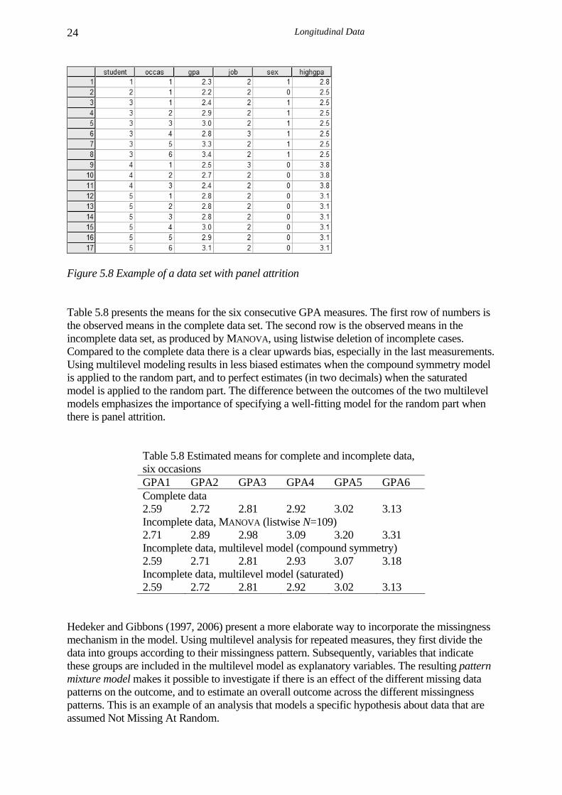
Longitudinal Data
24
Figure 5.8 Example of a data set with panel attrition Table 5.8 presents the means for the six consecutive GPA measures. The first row of numbers is the observed means in the complete data set. The second row is the observed means in the incomplete data set, as produced by MANOVA, using listwise deletion of incomplete cases. Compared to the complete data there is a clear upwards bias, especially in the last measurements. Using multilevel modeling results in less biased estimates when the compound symmetry model is applied to the random part, and to perfect estimates (in two decimals) when the saturated model is applied to the random part. The difference between the outcomes of the two multilevel models emphasizes the importance of specifying a well-fitting model for the random part when there is panel attrition.
Table 5.8 Estimated means for complete and incomplete data, six occasions GPA1 GPA2 GPA3 GPA4 GPA5 GPA6 Complete data 2.59 2.72 2.81 2.92 3.02 3.13 Incomplete data, MANOVA (listwise N=109) 2.71 2.89 2.98 3.09 3.20 3.31 Incomplete data, multilevel model (compound symmetry) 2.59 2.71 2.81 2.93 3.07 3.18 Incomplete data, multilevel model (saturated) 2.59 2.72 2.81 2.92 3.02 3.13
Hedeker and Gibbons (1997, 2006) present a more elaborate way to incorporate the missingness mechanism in the model. Using multilevel analysis for repeated measures, they first divide the data into groups according to their missingness pattern. Subsequently, variables that indicate these groups are included in the multilevel model as explanatory variables. The resulting pattern mixture model makes it possible to investigate if there is an effect of the different missing data patterns on the outcome, and to estimate an overall outcome across the different missingness patterns. This is an example of an analysis that models a specific hypothesis about data that are assumed Not Missing At Random.

Multilevel Analysis of Regression and Structural Equation Models 25
5.6.3 Accelerated designs One obvious issue in longitudinal studies is that the data collection process takes a long time. Given that multilevel analysis of longitudinal data does not assume that all subjects are measured on the same occasions, it is possible to speed up the process. Different age cohorts of subjects are followed for a relatively short period of time, and then a curve is modeled across the entire age span in the data. This is called a cohort-sequential design, or an accelerated design. Figure 5.9 illustrates this design.
Cohort 1 6 7 8 Cohort 2 7 8 9 Cohort 3 8 9 10 Total 6 7 8 9 10
Figure 5.9 Example of an accelerated design
In the cohort-sequential design depicted in Figure 5.9, there are three age cohorts of children who at the beginning of the study are 6, 7 and 8 years old, respectively. The data collection takes two years, with data collected from the same children yearly. In the total sample, we have an age range of 6–10, and we can fit a growth curve across 5 years, although the actual data collection takes only two years. The reading skill data presented in the section on varying occasions is another example of accelerated design. Although the data collection used 6 years, the age range in the sample is 6–14 years. In an accelerated design, the growth curve is estimated on a combination of cross-sectional and longitudinal information. Obviously, this assumes that the different cohorts are comparable, for example that in Figure 5.9 the 8–year olds in cohort 1 are comparable to the 8–year olds in cohort 3, who are in fact two years older than the children in cohort 1 and measured at a different measurement occasion. If the data collection contains a sufficient number of measurement occasions, this assumption can be tested, for example by fitting three separate linear growth curves and testing if these are equal in the three cohorts. Duncan, Duncan & Strycker (2006) provide a discussion of cohort-sequential designs and their analysis in the context of latent curve modeling, and Raudenbush and Chan (1993) discuss the analysis of cohort-sequential designs using multilevel regression models more closely. and Miyazaki and Raudenbush (2000) discuss tests for age×cohort interactions in accelerated designs. 5.6.4 The metric of time In section 5.2 the measurement occasions are numbered 0,…,5 to ensure that the intercept represents the starting point of the data collection. In section 5.3 on varying occasions, there are four measurement occasions, but instead of 0,…,3 the real ages of the children at these occasions are used, transformed so that the youngest recorded age (6 years) equals zero. This difference points toward a larger issue: what is the correct metric of time? Developmental models, for example growth curve models, are modeling a growth process that occurs in real time. The goal

Longitudinal Data
26
of such models is to estimate the overall growth pattern, and individual deviations from that pattern in the form of individual growth curves. Counting and indexing measurement occasions does not address these goals, using age-based models does. As discussed in the previous section on accelerated designs, age-based modeling is not unproblematic if subjects differ in age at the beginning of the data collection. On the one hand, this offers the means to analyze a wider age range than the number of years the data collection lasts, but on the other hand we must assume that there are no cohort effects. Especially when the initial age range is large, and the data collection period is short with respect to this age range, cohort effects can lead to misleading results. If there are cohort effects, it may be better to analyze the data ordered by data collection occasion, with differences in age at the first measurement occasion as predictors. A careful check of the assumption that there are no cohort effects is important in such cases. Setting the first measurement occasion to zero, or using a transformed age measure as the measure of time is not necessarily optimal. In the reading skill example in section 5.3, the age is transformed by subtracting six. This is reasonable; most children have some reading ability at that age. Using raw age is not reasonable, because in this metric the intercept represents reading skill at age zero, and the second level variance represents the variation in reading skill at age zero. These estimates are clearly meaningless. A similar example is the multilevel model for the development of speech in young children in Raudenbush and Bryk (2002). Here the age is given in months, and Raudenbush and Bryk subtract 12 because the average child starts to use words at about 12 months age. Deciding on the metric of time is not only a statistical problem; it is strongly connected to the topic of study. The major substantive problem is to establish a metric of time that fits the process. For example, in a study on the importance of a major life event, such as marriage or divorce, birth or death of a relative, the time of this event is often set to zero. This assumes that the event can be considered the start of the process that is examined. If the initial point is an event, age is often added as a subject level variable. This assumes that the curve after the event may differ for different age cohorts. Again, deciding on the metric of time is a substantive and theoretical issue, which cannot be settled by statistical reasoning alone. 5.7 SOFTWARE ISSUES The models that include complex covariance structures require multilevel software that allows restrictions on the random and fixed part. Some programs (HLM, SuperMix, Prelis, and the general packages SAS, SPSS and STATA) recognize the structure of longitudinal data, and allow direct specification of various types of autocorrelation structures. For a discussion of some of these structures in the context of multilevel longitudinal models see Hedeker and Gibbons (2006). If there are many different and differently spaced occasions, MANOVA and related models become impractical. With varying occasions, it is still possible to specify an autocorrelation structure, but it is more difficult to interpret than with fixed occasions. The program MLwiN can model very general autocorrelation structures using macros available from the Multilevel Modelling Project at the University of Bristol (Yang, Rasbash & Goldstein, 1998). Examples of such analyses are given by Goldstein, Healy and Rasbash (1994) and Barbosa and Goldstein (2000). It should be noted that many of these programs, when the time structure is generated automatically, number the occasions starting at one. Since this makes ‘zero’ a non-existent value for the measurement occasion variable, this is an unfortunate choice. If this happens, software users should override it with a choice that makes better sense given their substantive question.

1
14
Multilevel Factor Models The models described in the previous chapters are all multilevel variants of the conventional multiple regression model. This is not as restrictive as it may seem, since the multiple regression model is very flexible and can be used in many different applications (for detailed examples see Cohen & Cohen, 1983). Still, there are models that cannot be analyzed with multiple regression, notably factor analysis and path analysis models. A general approach that includes both factor and path analysis is Structural Equation Modeling, or SEM. The interest in structural equation modeling is generally on theoretical constructs, which are represented by the latent factors. The factor model, which is often called the measurement model, specifies how the latent factors are measured by the observed variables. The relationships between the theoretical constructs are represented by regression or path coefficients between the factors. The structural equation model implies a structure for the covariances between the observed variables, which explains the alternative name Covariance Structure Analysis. However, the model can be extended to include means of observed variables or factors in the model, which makes covariance structure analysis a less accurate name. Many researchers will simply think of these models as ‘Lisrel-models,’ which is also less accurate. LISREL is an abbreviation of LInear Structural RELations, and the name used by Jöreskog for one of the first and most popular SEM programs. Nowadays structural equation models need not be linear, and the possibilities of SEM extend well beyond the original LISREL program. Marcoulides and Schumacker (2001), for instance, discuss the possibility to fit nonlinear curves and interaction terms in SEM. Structural equation modeling is a general and convenient framework for statistical analysis that includes as special cases several traditional multivariate procedures, such as factor analysis, multiple regression analysis, discriminant analysis, and canonical correlation. Structural equation models are often visualized by a graphical path diagram. The statistical model is usually represented in a set of matrix equations. In the early seventies, when this technique was first introduced in social and behavioral research, the software usually required setups that specify the model in terms of these matrices. Thus, researchers had to distill the matrix representation from the path diagram, and provide the software with a series of matrices for the different sets of parameters, such as factor loadings and regression coefficients. A recent development is software that allows the researchers to specify the model directly as a path diagram. Since the focus in this chapter is on structural equation models for multilevel data, and not on structural equation modeling itself, the models will generally be introduced using path diagrams. Structural equation modeling has its roots in path analysis, which was invented by the geneticist Sewall Wright (Wright, 1921). It is customary to start a SEM analysis by drawing a path diagram. A path diagram consists of boxes and circles, which are connected by arrows. In Wright’s notation, observed (or measured) variables are represented by a rectangle or square box, and latent (or unmeasured) factors by a circle or ellipse. Single-headed arrows or ‘paths’ are used to define hypothesized causal relationships in the model, with the variable at the tail of the arrow being the cause of the variable at the point. Double-headed arrows indicate covariances or correlations, without a causal interpretation. Statistically, the single-headed arrows or paths represent regression coefficients, and double-headed arrows covariances.

Multilevel Factor Models
2
Often a distinction is made between the measurement model and the structural model. The measurement model, which is a confirmatory factor model, specifies how the latent factors are related to the observed variables. The structural model contains the relationships between the latent factors. In this chapter, I discuss multilevel factor analysis, and introduce the techniques currently available to estimate multilevel factor models. Multilevel path models, which are structural models that may or may not include latent factors, are discussed in Chapter Fifteen. For a general introduction in SEM, I refer to the introductory article by Hox and Bechger (1998) or introductory books such as Loehlin (2004) and Schumacker and Lomax (2004). A statistical treatment is presented by Bollen (1989). An interesting collection of introductory articles focusing on SEM models for multigroup and longitudinal data is found in Little, Schnabel and Baumert (2000). Structural equation models are often specified as models for the means and covariance matrix of multivariate normal data. The model is then
i iy μ η ε= + Λ + , (14.1) which states that the observed variables yi are predicted by a regression equation involving an intercept μ and the regression coefficients or loadings in factor matrix Λ multiplying the unobserved factor scores ηi plus a residual measurement error ε. This can then be expressed as a model for the covariance matrix Σ by '|Σ = ΛΦΛ +Θ , (14.2) where the covariance matrix Σ is expressed as a function of the factor matrix Λ, the matrix of covariances between factors Φ, and residual measurement errors in Θ. This chapter discusses two different appoaches to multilevel SEM. The first approach, described by Rabe-Hesketh, Skrondal and Zheng (2007) as the ‘within and between formulation’ focuses on determining separate estimates for the within (subject level) covariance matrix and the between (group level) covariance matrix. These are then modeled separately or simultaneously by an subject level (within) factor model and a group level (between) factor model, analogous to the single level equation given in 14.2. This works well, but has limitations, which will be discussed in the next section (14.1) that describes this approach in more detail. The second approach models the observed multilevel data directly with a model that includes variables at each available level and accommodates group-level variation of intercepts and slopes. It is the most accurate and versatile approach, but in some circumstances computationally demanding. It is also at the moment not widely available in standard multilevel or SEM software. This approach is described in section 14.2. 14.1 THE WITHIN AND BETWEEN APPROACH The within and between approach is based on an analysis of the subject level and the group level covariance matrix. This is in turn based on a decomposition of the variables to the available levels, which is discussed in the next section. 14.1.1 Decomposing multilevel variables Multilevel structural models assume that we have a population of individuals that are divided into groups. The individual data are collected in a p-variate vector Yig (subscript i for
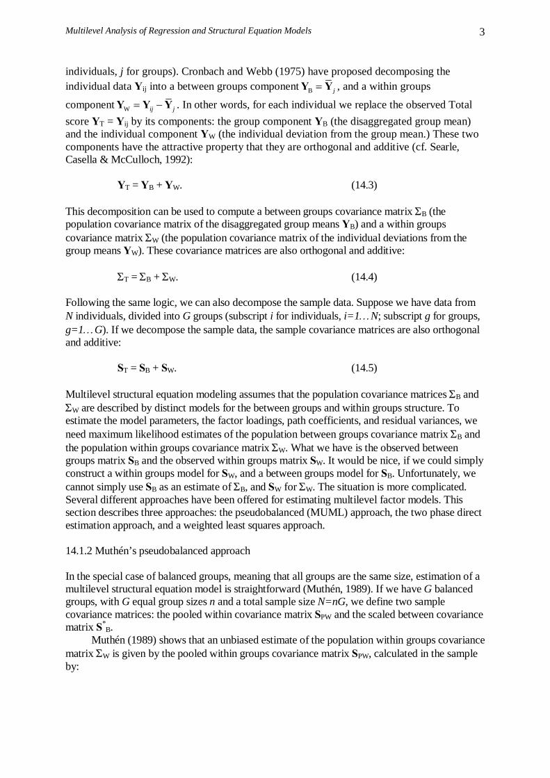
Multilevel Analysis of Regression and Structural Equation Models 3
individuals, j for groups). Cronbach and Webb (1975) have proposed decomposing the individual data Yij into a between groups component B j=Y Y , and a within groups
component W ij j= −Y Y Y . In other words, for each individual we replace the observed Total score YT = Yij by its components: the group component YB (the disaggregated group mean) and the individual component YW (the individual deviation from the group mean.) These two components have the attractive property that they are orthogonal and additive (cf. Searle, Casella & McCulloch, 1992): YT = YB + YW. (14.3) This decomposition can be used to compute a between groups covariance matrix ΣB (the population covariance matrix of the disaggregated group means YB) and a within groups covariance matrix ΣW (the population covariance matrix of the individual deviations from the group means YW). These covariance matrices are also orthogonal and additive: ΣT = ΣB + ΣW. (14.4) Following the same logic, we can also decompose the sample data. Suppose we have data from N individuals, divided into G groups (subscript i for individuals, i=1…N; subscript g for groups, g=1…G). If we decompose the sample data, the sample covariance matrices are also orthogonal and additive: ST = SB + SW. (14.5) Multilevel structural equation modeling assumes that the population covariance matrices ΣB and ΣW are described by distinct models for the between groups and within groups structure. To estimate the model parameters, the factor loadings, path coefficients, and residual variances, we need maximum likelihood estimates of the population between groups covariance matrix ΣB and the population within groups covariance matrix ΣW. What we have is the observed between groups matrix SB and the observed within groups matrix SW. It would be nice, if we could simply construct a within groups model for SW, and a between groups model for SB. Unfortunately, we cannot simply use SB as an estimate of ΣB, and SW for ΣW. The situation is more complicated. Several different approaches have been offered for estimating multilevel factor models. This section describes three approaches: the pseudobalanced (MUML) approach, the two phase direct estimation approach, and a weighted least squares approach. 14.1.2 Muthén’s pseudobalanced approach In the special case of balanced groups, meaning that all groups are the same size, estimation of a multilevel structural equation model is straightforward (Muthén, 1989). If we have G balanced groups, with G equal group sizes n and a total sample size N=nG, we define two sample covariance matrices: the pooled within covariance matrix SPW and the scaled between covariance matrix S*
B. Muthén (1989) shows that an unbiased estimate of the population within groups covariance matrix ΣW is given by the pooled within groups covariance matrix SPW, calculated in the sample by:

Multilevel Factor Models
4
( )( )G n
ij j ij jj i
PW N G
′− −
=−
∑∑ Y Y Y YS (14.6)
Equation (14.6) corresponds to the conventional equation for the covariance matrix of the individual deviation scores, with N-G in the denominator instead of the usual N-1. Since the pooled within groups covariance matrix SPW is an unbiased estimate of the population within groups covariance matrix ΣW, we can estimate the population within group structure directly by constructing and testing a model for SPW. The scaled between groups covariance matrix for the disaggregated group means *
BS , calculated in the sample, is given by:
( )( )
*
1
G
j jj
B
n
G
′− −
=−
∑ Y Y Y YS . (14.7)
Muthén (1989, 1990) shows that SPW is the maximum likelihood estimator of ΣW, with sample size N-G, and S*
B is the maximum likelihood estimator of the composite ΣW + cΣB, with sample size G, and c equal to the common group size n: PW W=S Σ (14.8) and *
B W Bc= +S Σ Σ . (14.9) Equations 14.8 and 14.9 suggest using the multi-group option of conventional SEM software for a simultaneous analysis at both levels. However, if we model the between groups structure, we cannot simply construct and test a simple model for ΣB, because *
BS estimates a combination of ΣW and ΣB. Instead, we have to specify for the *
BS ‘group’ a model that contains two distinct sub-models: one for the within structure and one for the between structure. The procedure is that we specify two groups, with covariance matrices SPW and *
BS (based on N-G and G observations). The model for ΣW must be specified for both SPW and *
BS , with equality restrictions between both ‘groups’ to guarantee that we are indeed estimating the same model in both covariance matrices, and the model for ΣB is specified for *
BS only, with the scale factor c built into the model. The reasoning strictly applies only in the so-called balanced case, that is, if all groups have the same group size. In the balanced case, the scale factor c is equal to the common group size n. The unbalanced case, where the group sizes differ, with G groups of unequal sizes, is more complicated. In this case, SPW is still the maximum likelihood estimator of ΣW, but *
BS now estimates a different expression for each set of groups with distinct group size d: *
Bd W d Bc= +S Σ Σ , (14.10) where equation 14.10 holds for each distinct set of groups with a common group size equal to nd, and cd=nd (Muthén, 1990, 1994). Full Information Maximum Likelihood (FIML) estimation for

Multilevel Analysis of Regression and Structural Equation Models 5
unbalanced groups implies specifying a separate between-group model for each distinct group size. These between groups models have different scaling parameters cd for each distinct group size, and require equality constraints across all other parameters and inclusion of a mean structure (Muthén, 1994, p. 385). Thus, using conventional SEM software for unbalanced data requires a complicated modeling scheme that creates a different ‘group’ for each set of groups with the same group size. This results in large and complex models, with possibly groups with a sample size less than the number of elements in the corresponding covariance matrix. This makes full Maximum Likelihood estimation problematic, and therefore Muthén (1989, 1990) proposes to ignore the unbalance, and to compute a single S*
B. The model for S*B includes an ad
hoc estimator c* for the scaling parameter, which is close to the average sample size:
( )
2 2
*
1
G
jj
N nc
N G
−=
−
∑. (14.11)
The result is a limited information Maximum Likelihood solution, which McDonald (1994) calls a pseudobalanced solution, and Muthén (1989, 1994) the MUML (for MUthén’s ML) solution.
Figure 6.1 presents a path diagram for the pseudobalanced model. Left in the figure is the within model for the pooled within matrix. Right in the diagram is the model for the scaled between matrix. It repeats the model for the within matrix, with equality constraints across all corresponding parameters. On top of this, for each variable a corresponding between variable is specified. These between level variables are latent variables representing the second or between level intercept variances. C is the scaling constant. The between level model is constructed for the latent between variables.
Figure 14.1 Path diagram for pseudobalanced model
Muthén (1989, 1990) shows that *
BS is a consistent and unbiased estimator of the composite ΣW + cΣB. This means that with large samples (of both individuals and groups!) *
BS is a close estimate of ΣB, and the pseudobalanced solution produces a good approximation given adequate sample sizes. Simulation studies (Hox and Maas, 2001a; Hox, Maas & Brinkuis, 2008) find that the within groups part of the model poses no problems in any of the simulated conditions. In the between groups part of the model, the factor loadings are generally accurate. However, the

Multilevel Factor Models
6
residual variances are underestimated, and the standard errors are generally too small, leading to an operating alpha level of about 8%. In addition, the chi-square model test is rejected too often, which again results in an operating alpha level of about 8%. Yuan and Hayashi (2005) show analytically that MUML standard errors and chi-square tests lead to correct inferences when the between level sample size goes to infinity and the coefficient of variation of the group sizes goes to zero. Both simulations and analytical work agree that larger sample sizes do not improve the accuracy with unbalanced data. So, with severely unbalanced data, MUML produces biased standard errors and significance tests, and this bias is not diminished when the sample size is increased. Since the pseudobalanced approach needs the within groups model both for the pooled within groups and the scaled between groups model, and needs to incorporate the scaling factor for the between groups model, the actual model can become quite complicated. Most modern structural equation software includes the MUML approach for two-level data, generally combined with default robust estimators for the standard errors and the chi-square test statistic to correct for the remaining heterogeneity (cf. Muthén & Satorra, 1995). The complications of the setup are generally hidden for the user. In software that does not include MUML as an option, it is still possible to calculate SPW and SB separately, and constructing the complicated setup. For details I refer to Hox (1993) and the first edition of this book (Hox, 2002). 14.1.3 Direct estimation of the within and between matrix Goldstein (1987, 2003) has suggested using the multivariate multilevel model described in Chapter Ten to produce a covariance matrix at the different levels, and to input these into a standard SEM program for further analysis. For our family data, we would use a multivariate multilevel model with three separate levels for the six intelligence tests, the individual children, and the families. We create six dummy variables to indicate the six intelligence scales, and exclude the intercept from the model. Hence, at the lowest level (the variables level) we have 1 1 2 2 6 6hij ij ij ij ij ij ijY d d dπ π π= + +…+ , (14.12) at the individual level we have pij pj pijuπ β= + , (14.13) and at the family level (the third level in the multivariate model), we have pj p pjuβ γ= + . (14.14) By substitution we obtain
1 1 2 2
1 1 2 2 1 1 2 2
hij ij ij p pij
ij ij ij ij pij pij j ij j ij pj pij
Y d d d
u d u d u d u d u d u d
γ γ γ= + +…+
+ + +…+ + + +…+. (14.15)
In sum notation, we have
6 6 6
1 1 1hij h hij hij hij hj hij
h h hY d u d u dγ
= = =
= + +∑ ∑ ∑ . (14.16)

Multilevel Analysis of Regression and Structural Equation Models 7
The model described by equation (14.16) provides us with estimates of the six test means, and of their variances and covariances at the individual and family level. Since in this application we are mostly interested in the variances and covariances, RML estimation is preferred to FML estimation. The individual level (within) covariances and the family level (between) covariances and means are direct maximum likelihood estimators of their population counterparts, which can be input to any SEM software, either separately or in a two-group analysis. Hox and Maas (2004) explain this approach in more detail.
The fact that the individual level (within families) and family level (between families) covariances are estimated directly, and consequently can be modeled directly and separately by any SEM program, is a distinct advantage of the multivariate multilevel approach. As a result, we get separate model tests and fit indices at all levels. The multivariate multilevel approach to multilevel SEM also generalizes straightforwardly to more than two levels. There are other advantages as well. First, since the multilevel multivariate model does not assume that we have a complete set of variables for each individual, incomplete data are accommodated without special effort. Second, if we have dichotomous or ordinal variables, we can use the multilevel generalized linear model to produce the covariance matrices, again without special effort. There are some disadvantages to the multivariate multilevel approach as well. An important disadvantage is that the covariances produced by the multivariate multilevel approach are themselves estimated values. They are not directly calculated, as the pooled within groups and scaled between groups covariances are, but they are estimates produced by a complex statistical procedure. The estimation in the second step treats these estimates as data or observed covariance matrices. If the data have a multivariate normal distribution, the within groups and between groups covariances can be viewed as observed values, which have a known sampling distribution. However, when we have incomplete data it is unclear what the proper sample size is, and in the case of non-normal (e.g., dichotomous or ordinal) variables we know that the sampling distribution is not normal. Since the normal sampling distribution is used by SEM programs to calculate the chi-square model test and the standard errors of the parameter estimates, the chi-square test and standard errors cannot be trusted unless data are complete and multivariate normal. 14.1.4 Analysis of the within and between matrix using weighted least squares Asparouhov and Muthén (2007) describe an approach to multilevel SEM that uses separate estimation of the covariance matrices followed by an estimation method that overcomes the problems that are encountered with direct estimation of the within and between covariance matrix with non-normal data. In this approach, univariate maximum likelihood methods are used to estimate the vector of means μ at the between group level, and the diagonal elements (the variances) of SW and SB. In the case of ordinal categorical variables, thresholds are estimated as well. Next, the off-diagonal elements of SW and SB are estimated using bivariate maximum likelihood methods. Finally, the asymptotic variance-covariance matrix for these estimates is obtained, and the multilevel SEM is estimated for both levels using Weighted Least Squares (WLS). Currently, this approach is only available in Mplus.
WLS is an estimation method that uses the variance-covariance matrix of SW and SB as a weight matrix to obtain correct chi-squares and standard errors. This estimation method is developed for efficient estimation of multilevel models with non-normal variables, since for such data full maximum likelihood estimation requires high-dimensional numerical integration, which is computationally very demanding. Multilevel WLS can also be used for multilevel estimation with continuous variables, but then it does not have a real advantage. Standard WLS uses a weight matrix based on the asymptotic covariances of all estimated parameters. For the unrestricted model, the number of parameters is large, and the asymptotic
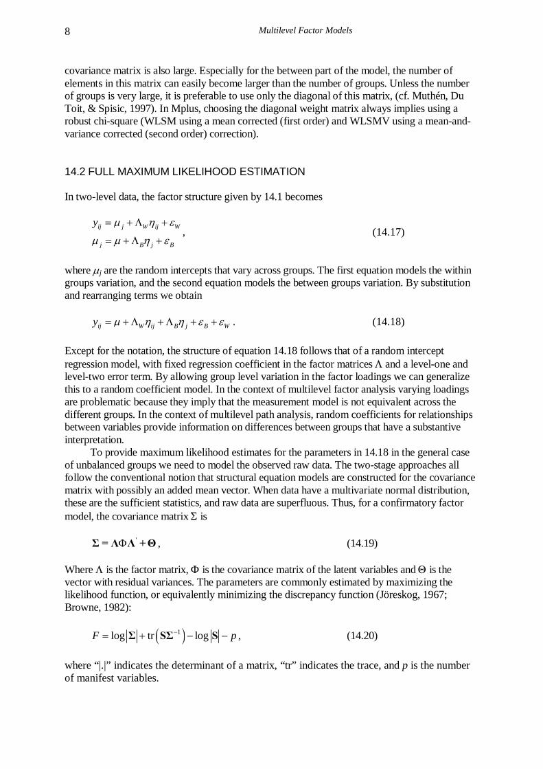
Multilevel Factor Models
8
covariance matrix is also large. Especially for the between part of the model, the number of elements in this matrix can easily become larger than the number of groups. Unless the number of groups is very large, it is preferable to use only the diagonal of this matrix, (cf. Muthén, Du Toit, & Spisic, 1997). In Mplus, choosing the diagonal weight matrix always implies using a robust chi-square (WLSM using a mean corrected (first order) and WLSMV using a mean-and-variance corrected (second order) correction). 14.2 FULL MAXIMUM LIKELIHOOD ESTIMATION In two-level data, the factor structure given by 14.1 becomes
ij j W ij W
j B j B
y μ η ε
μ μ η ε
= + Λ +
= + Λ +, (14.17)
where μj are the random intercepts that vary across groups. The first equation models the within groups variation, and the second equation models the between groups variation. By substitution and rearranging terms we obtain
ij W ij B j B Wy μ η η ε ε= + Λ + Λ + + . (14.18) Except for the notation, the structure of equation 14.18 follows that of a random intercept regression model, with fixed regression coefficient in the factor matrices Λ and a level-one and level-two error term. By allowing group level variation in the factor loadings we can generalize this to a random coefficient model. In the context of multilevel factor analysis varying loadings are problematic because they imply that the measurement model is not equivalent across the different groups. In the context of multilevel path analysis, random coefficients for relationships between variables provide information on differences between groups that have a substantive interpretation. To provide maximum likelihood estimates for the parameters in 14.18 in the general case of unbalanced groups we need to model the observed raw data. The two-stage approaches all follow the conventional notion that structural equation models are constructed for the covariance matrix with possibly an added mean vector. When data have a multivariate normal distribution, these are the sufficient statistics, and raw data are superfluous. Thus, for a confirmatory factor model, the covariance matrix Σ is 'ΦΣ = Λ Λ +Θ , (14.19) Where Λ is the factor matrix, Φ is the covariance matrix of the latent variables and Θ is the vector with residual variances. The parameters are commonly estimated by maximizing the likelihood function, or equivalently minimizing the discrepancy function (Jöreskog, 1967; Browne, 1982): ( )1log tr logF p−= + − −Σ SΣ S , (14.20) where “|.|” indicates the determinant of a matrix, “tr” indicates the trace, and p is the number of manifest variables.

Multilevel Analysis of Regression and Structural Equation Models 9
Unbalanced groups can be viewed as a form of incomplete data. For incomplete data, the maximum likelihood approach defines the model and the likelihood in terms of the raw data, which is why it is sometimes called the raw likelihood method. Raw ML minimizes the function (Arbuckle, 1996):
( ) ( )' 1
1 1log log -
N N
i i i i i ii i
F −
= =
= +∑ ∑Σ x -μ Σ x μ , (14.21)
where the subscript i refers to the observed cases, xi to the variables observed for case i, and μi and Σi contain the population means and covariances of the variables observed for case i. If the data are complete, equations 14.20 and 14.21 are equivalent. If the data are incomplete, the covariance matrix is no longer a sufficient statistic, and minimizing the discrepancy function given by 14.21 provides the maximum likelihood estimates for the incomplete data. Mehta and Neale (2005) show that models for multilevel data, with individuals nested within groups, can be expressed as a structural equation model. The fit function given by equation (14.21) applies, with clusters as units of observation, and individuals within clusters as variables. Unbalanced data, here unequal numbers of individuals within clusters, are included the same way as incomplete data in standard SEM. While the two-stage approaches (MUML, direct estimation and WLS) include only random intercepts in the between groups model, the ML representation can incorporate random slopes as well (Mehta & Neale, 2005). In theory, any modern SEM software that allows for incomplete data can be used to estimate multilevel SEM. In practice, specialized software is used that makes use of the specific multilevel structure in the data to simplify calculations. Full maximum likelihood multilevel SEM is currently available for two-level models in Mplus and for many-level models in GLLAMM. A recent development is to use robust standard errors and chi-squares for significance testing. With multilevel data, robust chi-squares and standard errors offer some protection against unmodeled heterogeneity, which may result from misspecifying the group level model, or by omitting a level. Finaly, Skrondal and Rabe-Hesketh (2004) show how to combine this with a generalized linear model for the observed variables, which allows for non-normal variables. This is currently available only in Mplus and GLLAMM.
The next section analyzes an example data set, using all four estimation methods discussed above. When all methods are compared, the pseudobalanced MUML approach and the multivariate multilevel two stage estimation method are the least accurate, especially for the between model estimates. These methods are clearly outdated. Simulations (Hox, Maas & Brinkhuis, 2008) have shown that both WLS and full ML estimation are more accurate than MUML, and that the difference between WLS and ML is negligible. Our example confirms that ML and WLS are quite similar. When ML estimation is possible, it is the method of choice, but when the demands for ML estimation overtax the computer capacity, WLS is a viable alternative. The maximum likelihood approach is the only approach that allows random slopes in the model. In a confirmatory factor analysis, this means that factor loadings are allowed to vary across groups. In our example, none of the six individual-level factor loadings has significant slope variation across families. In confirmatory factor analysis this is desirable, because finding varying factor loadings implies that the scales involved are not measuring the same thing in the same way across families. Varying slopes in a measurement model indicate lack of measurement equivalence across groups. 14.3 AN EXTENDED EXAMPLE OF MULTILEVEL FACTOR ANALYSIS
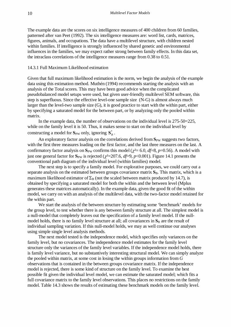
Multilevel Factor Models
10
The example data are the scores on six intelligence measures of 400 children from 60 families, patterned after van Peet (1992). The six intelligence measures are: word list, cards, matrices, figures, animals, and occupations. The data have a multilevel structure, with children nested within families. If intelligence is strongly influenced by shared genetic and environmental influences in the families, we may expect rather strong between family effects. In this data set, the intraclass correlations of the intelligence measures range from 0.38 to 0.51. 14.3.1 Full Maximum Likelihood estimation Given that full maximum likelihood estimation is the norm, we begin the analysis of the example data using this estimation method. Muthén (1994) recommends starting the analysis with an analysis of the Total scores. This may have been good advice when the complicated pseudobalanced model setups were used, but given user-friendly multilevel SEM software, this step is superfluous. Since the effective level-one sample size (N-G) is almost always much larger than the level-two sample size (G), it is good practice to start with the within part, either by specifying a saturated model for the between part, or by analyzing only the pooled within matrix. In the example data, the number of observations on the individual level is 275-50=225, while on the family level it is 50. Thus, it makes sense to start on the individual level by constructing a model for SPW only, ignoring *
BS . An exploratory factor analysis on the correlations derived from SPW suggests two factors, with the first three measures loading on the first factor, and the last three measures on the last. A confirmatory factor analysis on SPW confirms this model (χ²= 6.0, df=8, p=0.56). A model with just one general factor for SPW is rejected (χ²=207.6, df=9, p<0.001). Figure 14.1 presents the conventional path diagram of the individual level (within families) model.
The next step is to specify a family model. For explorative purposes, we could carry out a separate analysis on the estimated between groups covariance matrix SB. This matrix, which is a maximum likelihood estimator of ΣB (not the scaled between matrix produced by 14.7), is obtained by specifying a saturated model for both the within and the between level (Mplus generates these matrices automatically). In the example data, given the good fit of the within model, we carry on with an analysis of the multilevel data, with the two-factor model retained for the within part.
We start the analysis of the between structure by estimating some ‘benchmark’ models for the group level, to test whether there is any between family structure at all. The simplest model is a null-model that completely leaves out the specification of a family level model. If the null-model holds, there is no family level structure at all; all covariances in SB are the result of individual sampling variation. If this null-model holds, we may as well continue our analyses using simple single level analysis methods. The next model tested is the independence model, which specifies only variances on the family level, but no covariances. The independence model estimates for the family level structure only the variances of the family level variables. If the independence model holds, there is family level variance, but no substantively interesting structural model. We can simply analyze the pooled within matrix, at some cost in losing the within groups information from G observations that is contained in the between groups covariance matrix. If the independence model is rejected, there is some kind of structure on the family level. To examine the best possible fit given the individual level model, we can estimate the saturated model; which fits a full covariance matrix to the family level observations. This places no restrictions on the family model. Table 14.3 shows the results of estimating these benchmark models on the family level.

Multilevel Analysis of Regression and Structural Equation Models 11
Table 14.1. Family level benchmark models Family model Chi-square df p Null 323.6 29 .00 Independence 177.2 23 .00 Saturated 6.7 8 .57
The null model and the independence model are both rejected. Subsequently, we specify for the family level the same one-factor and two-factor models we have used at the individual level. The one-factor model fits well (χ²=11.9, df=17, p=0.80). The two-factor model is no improvement (difference chi-square 0.15, p=0.70).
The principle of using the simplest model that fits well leads to acceptance of the one factor model on the family level. The chi-square model test is not significant, and the fit indices are fine: CFI is 1.00 and the RMSEA is 0.00. Figure 14.2 presents the within and between model in a single path diagram. Note that, consistent with the full path diagram in Figure 14.3, the between level variables that represent the family level intercept variance of the observed variables, are latent variables, depicted by circles or ellipses.
Figure 14.2 Diagram for family IQ data 1
Using the maximum likelihood method (ML) in Mplus leads to the estimates reported in Table 14.2.
Table 14.2 Individual and family level estimates, ML estimation Individual level Family level Numer. Percept. resid. var. General resid. var.
Wordlst 3.18 (.20) 6.19 (.74) 3.06 (.39) 1.25 (.57)
Cards 3.14 (.19) 5.40 (.69) 3.05 (.39) 1.32 (.59)
Matrix 3.05 (.20) 6.42 (.71) 2.63 (.38) 1.94 (.67)

Multilevel Factor Models
12
Figures 3.10 (.20) 6.85 (.76) 2.81 (.40) 2.16 (.71)
Animals 3.19 (.19) 4.88 (.70) 3.20 (.38) 0.66 (.49)
Occupat 2.78 (.18) 5.33 (.60) 3.44 (.42) 1.58 (.62)
Standard errors in parentheses. Correlation between individual factors: 0.38.
14.3.2 Weighted Least Squares estimation Using the separate estimation/WLS method with robust chi-square (WLSMV) in Mplus leads to the estimates reported in Table 14.7.1 The chi-square model test accepts the model (χ²=5.91, df=7, p=0.55), the fit indices are good: CFI is 1.00 and the RMSEA is 0.00. The parameter estimates in Table 14.3 are similar to the full Maximum Likelihood estimates, but not identical. The robust standard errors lead to the same conclusions as the asymptotic standard errors used with full Maximum Likelihood estimation.
Table 14.3 Individual and family level estimates, WLS estimation Individual level Family level Numer. Percept. resid. var. General resid. var.
Wordlst 3.25 (.15) 5.67 (.84) 3.01 (.48) 1.51 (.62)
Cards 3.14 (.18) 5.44 (.68) 3.03 (.38) 1.25 (.71)
Matrix 2.96 (.22) 6.91 (.92) 2.62 (.45) 2.02 (.69)
Figures 2.96 (.22) 7.67 (.92) 2.80 (.46) 2.03 (.72)
Animals 3.35 (.21) 3.79 (.99) 3.15 (.41) 0.96 (.61)
Occupat 2.75 (.24) 5.49 (.94) 3.43 (.44) 1.67 (.63)
Standard errors in parentheses. Correlation between individual factors: 0.38.
14.3.3 Direct estimation of the within and between matrix followed by separate modeling Since the family example data are multivariate normal and complete, the direct estimation method discusses in section 14.2.3 is a viable option. Covariance matrices were estimated for the within and the between part using the multivariate multilevel model presented in Chapter Ten. Estimation was carried out in MLwiN Restricted Maximum Likelihood; subsequent SEM modeling was done in Amos. The within model does fits well: χ²=6.9, df=8, p=.55, CFI is 1.00 and the RMSEA is 0.00. Analysis of the between matrix produces inconsistent results: χ²=15.8, df=9, p<.07, CFI is 0.99 but the RMSEA is 0.11. The parameter estimates for the model are presented in Table 14.4.
Table 14.4 Individual and family level estimates, MUML estimation 1 The asymptotic chi-square is available by specifying full WLS estimation. As explained earlier, this leads to a very large weight matrix. With a group level sample size of only 60 this is a recipe for disaster, hence the choice for a robust WLS estimation.
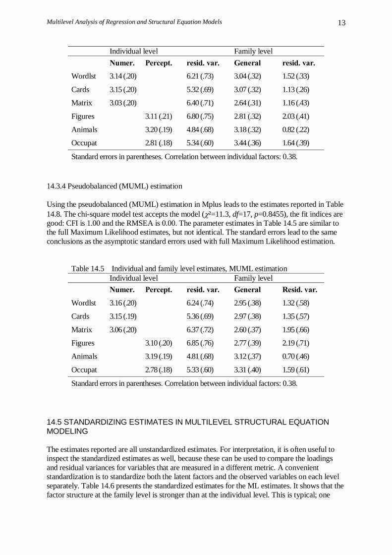
Multilevel Analysis of Regression and Structural Equation Models 13
Individual level Family level Numer. Percept. resid. var. General resid. var.
Wordlst 3.14 (.20) 6.21 (.73) 3.04 (.32) 1.52 (.33)
Cards 3.15 (.20) 5.32 (.69) 3.07 (.32) 1.13 (.26)
Matrix 3.03 (.20) 6.40 (.71) 2.64 (.31) 1.16 (.43)
Figures 3.11 (.21) 6.80 (.75) 2.81 (.32) 2.03 (.41)
Animals 3.20 (.19) 4.84 (.68) 3.18 (.32) 0.82 (.22)
Occupat 2.81 (.18) 5.34 (.60) 3.44 (.36) 1.64 (.39)
Standard errors in parentheses. Correlation between individual factors: 0.38.
14.3.4 Pseudobalanced (MUML) estimation Using the pseudobalanced (MUML) estimation in Mplus leads to the estimates reported in Table 14.8. The chi-square model test accepts the model (χ²=11.3, df=17, p=0.8455), the fit indices are good: CFI is 1.00 and the RMSEA is 0.00. The parameter estimates in Table 14.5 are similar to the full Maximum Likelihood estimates, but not identical. The standard errors lead to the same conclusions as the asymptotic standard errors used with full Maximum Likelihood estimation.
Table 14.5 Individual and family level estimates, MUML estimation Individual level Family level Numer. Percept. resid. var. General Resid. var.
Wordlst 3.16 (.20) 6.24 (.74) 2.95 (.38) 1.32 (.58)
Cards 3.15 (.19) 5.36 (.69) 2.97 (.38) 1.35 (.57)
Matrix 3.06 (.20) 6.37 (.72) 2.60 (.37) 1.95 (.66)
Figures 3.10 (.20) 6.85 (.76) 2.77 (.39) 2.19 (.71)
Animals 3.19 (.19) 4.81 (.68) 3.12 (.37) 0.70 (.46)
Occupat 2.78 (.18) 5.33 (.60) 3.31 (.40) 1.59 (.61)
Standard errors in parentheses. Correlation between individual factors: 0.38. 14.5 STANDARDIZING ESTIMATES IN MULTILEVEL STRUCTURAL EQUATION MODELING The estimates reported are all unstandardized estimates. For interpretation, it is often useful to inspect the standardized estimates as well, because these can be used to compare the loadings and residual variances for variables that are measured in a different metric. A convenient standardization is to standardize both the latent factors and the observed variables on each level separately. Table 14.6 presents the standardized estimates for the ML estimates. It shows that the factor structure at the family level is stronger than at the individual level. This is typical; one
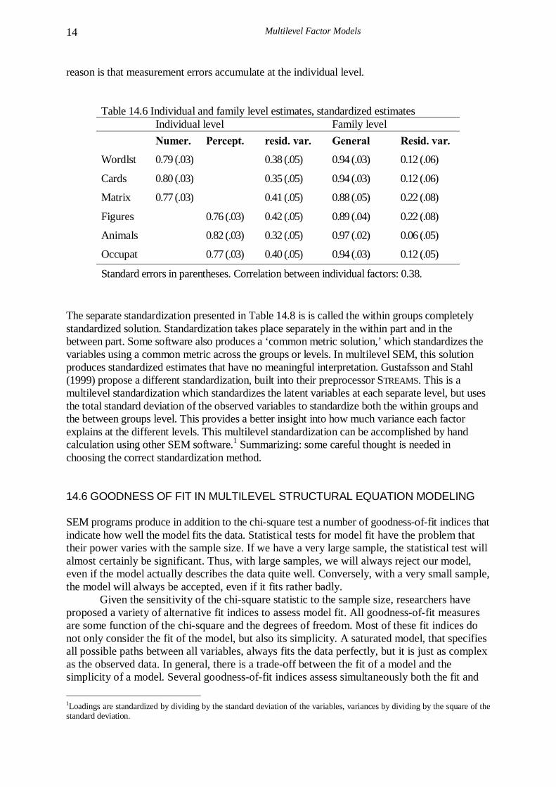
Multilevel Factor Models
14
reason is that measurement errors accumulate at the individual level.
Table 14.6 Individual and family level estimates, standardized estimates Individual level Family level Numer. Percept. resid. var. General Resid. var.
Wordlst 0.79 (.03) 0.38 (.05) 0.94 (.03) 0.12 (.06)
Cards 0.80 (.03) 0.35 (.05) 0.94 (.03) 0.12 (.06)
Matrix 0.77 (.03) 0.41 (.05) 0.88 (.05) 0.22 (.08)
Figures 0.76 (.03) 0.42 (.05) 0.89 (.04) 0.22 (.08)
Animals 0.82 (.03) 0.32 (.05) 0.97 (.02) 0.06 (.05)
Occupat 0.77 (.03) 0.40 (.05) 0.94 (.03) 0.12 (.05)
Standard errors in parentheses. Correlation between individual factors: 0.38. The separate standardization presented in Table 14.8 is is called the within groups completely standardized solution. Standardization takes place separately in the within part and in the between part. Some software also produces a ‘common metric solution,’ which standardizes the variables using a common metric across the groups or levels. In multilevel SEM, this solution produces standardized estimates that have no meaningful interpretation. Gustafsson and Stahl (1999) propose a different standardization, built into their preprocessor STREAMS. This is a multilevel standardization which standardizes the latent variables at each separate level, but uses the total standard deviation of the observed variables to standardize both the within groups and the between groups level. This provides a better insight into how much variance each factor explains at the different levels. This multilevel standardization can be accomplished by hand calculation using other SEM software.1 Summarizing: some careful thought is needed in choosing the correct standardization method. 14.6 GOODNESS OF FIT IN MULTILEVEL STRUCTURAL EQUATION MODELING SEM programs produce in addition to the chi-square test a number of goodness-of-fit indices that indicate how well the model fits the data. Statistical tests for model fit have the problem that their power varies with the sample size. If we have a very large sample, the statistical test will almost certainly be significant. Thus, with large samples, we will always reject our model, even if the model actually describes the data quite well. Conversely, with a very small sample, the model will always be accepted, even if it fits rather badly.
Given the sensitivity of the chi-square statistic to the sample size, researchers have proposed a variety of alternative fit indices to assess model fit. All goodness-of-fit measures are some function of the chi-square and the degrees of freedom. Most of these fit indices do not only consider the fit of the model, but also its simplicity. A saturated model, that specifies all possible paths between all variables, always fits the data perfectly, but it is just as complex as the observed data. In general, there is a trade-off between the fit of a model and the simplicity of a model. Several goodness-of-fit indices assess simultaneously both the fit and 1Loadings are standardized by dividing by the standard deviation of the variables, variances by dividing by the square of the standard deviation.

Multilevel Analysis of Regression and Structural Equation Models 15
the simplicity of a model. The goal is to produce a goodness-of-fit index that does not depend on the sample size or the distribution of the data. In fact, simulations have shown that most goodness-of-fit indices still depend on sample size and distribution, but the dependency is much smaller than that of the routine chi-square test.
Most SEM software computes a bewildering array of goodness-of-fit indices. All of them are functions of the chi-square statistic, but some include a second function that penalizes complex models. For instance, Akaike’s information criterion (AIC) is twice the chi-square statistic minus the degrees of freedom for the model. For a detailed review and evaluation of a large number of fit indices, including those mentioned here, I refer to Gerbing and Anderson (1993).
Jöreskog and Sörbom (1989) have introduced two goodness-of-fit indices called GFI (Goodness of Fit) and AGFI (Adjusted GFI). The GFI indicates goodness-of-fit, and the AGFI attempts to adjust the GFI for the complexity of the model. Bentler (1990) has introduced a similar index called the Comparative Fit Index CFI. Two other well-known fit measures are the Tucker-Lewis Index TLI (Tucker & Lewis, 1973), also known as the Non-Normed Fit Index or NNFI, and the Normed Fit Index NFI (Bentler & Bonett, 1980). Both the NNFI and the NFI adjust for complexity of the model. Simulation research shows that all these indices still depend on sample size and estimation method (e.g., ML or GLS), with the CFI and the TLI/NNFI showing the best overall performance (Chou & Bentler, 1995; Kaplan, 1995). If the model fits perfectly, these fit indices should have the value 1. Usually, a value of at least 0.90 is required to accept a model, while a value of at least 0.95 is required to judge the model fit as ‘good.’ However, these are just rules of thumb. A different approach to model fit is to accept that models are only approximations, and that perfect fit may be too much to ask for. Instead, the problem is to assess how well a given model approximates the true model. This view led to the development of an index called RMSEA, for Root Mean Square Error of Approximation (Browne & Cudeck, 1992). If the approximation is good, the RMSEA should be small. Typically, a RMSEA of less than 0.08 is required (Kline, 2004), with RMSEA less than 0.05 is required to judge the model fit as ‘good’. Statistical tests or confidence intervals can be computed to test if the RMSEA is significantly larger than this lower bound. Given the many possible goodness-of-fit indices, the customary advice is to assess fit by inspecting several fit indices that derive from different principles. Therefore, for the confirmatory factor model for the family data, I have reported the chi-square test, and the fit indices CFI and RMSEA. A general problem with these goodness-of-fit indices in multilevel SEM is that they apply to the entire model. Therefore, the goodness-of-fit indices reflect both the degree of fit in the within model and in the between model. Since the sample size for the within ‘group’ is generally the largest, this part of the model dominates the value of the fit indices. Clearly, it makes sense to assess the fit for both parts of the model separately. Since the within groups sample size is usually much larger than the between groups sample size, we do not lose much information if we model the within groups matrix separately, and interpret the fit indices produced in this analysis separately. A simple way to obtain goodness-of-fit indices for the between model is to specify a saturated model for the within groups level. The saturated model estimates all covariances between all variables. It has no degrees of freedom, and always fits the data perfectly. As a result, the degree of fit indicated by the goodness-of-fit indices, represents the (lack of) fit of the between model. This is not the best way to assess the fit of the between model, because the perfect fit of the within model also influences the value of the fit index. Fit indices that are mostly sensitive to the degree of fit will show a spuriously good fit, while fit indices that also reflect the parsimony of the model may show a spurious lack of fit.

Multilevel Factor Models
16
A better way to indicate the fit of the within and between model separately is to calculate these by hand. Most fit indices are a simple function of the chi-square, sample size N, and degrees of freedom df. Some consider only the current model, the target model Mt, others also consider a baseline model, usually the independence model MI. By estimating the independence and the target model for the within matrix, with a saturated model for the between matrix, we can assess how large the contribution to the overall chi-square is for the various within models. In the same way, by estimating the independence and the target model for the between matrix, with a saturated model for the within matrix, we can assess how large the contribution to the overall chi-square is for the various between models. Using this information, we can calculate the most common goodness-of-fit indices. Most SEM software produces the needed information, and the references and formulas are in the user manuals and in the general literature (e.g., Gerbing & Anderson, 1992).
Table 14.7 gives the separate chi-squares, degrees of freedom, and sample sizes for the independence model and the final model for the family intelligence example.
Table 14.7 Chi-squares and df separate for individual and family level models
Individual level, Between model saturated
Family level, Within model saturated
independence 2 factors independence 1 factor
chi-square 805.51 6.72 168.88 4.74
Df 30 8 15 9
N 340 340 60 60 The comparative fit index CFI (Bentler, 1990) is given by
2
21 t t
I I
dfCFI
dfχχ
−= −
−. (14.22)
In equation (14.18), 2
tχ is the chi-square of the target model, 2Iχ is the chi-square for the
independence model, and dft and dfI are the degrees of freedom for the target and the independence model. If the difference of the chi-square and the degrees of freedom is negative, it is replaced by zero. So, for example, the CFI for the family level model is given by
( ) ( )1 4.74 9 168.88 15 1 0 /153.88 1.00CFI = − − − = − = . The Tucker-Lewis index, TLI, which is also known as the Non-Normed Fit Index, NNFI, is given by
22
2
1
tI
I t
I
I
df dfTLI
df
χχ
χ
−=
−. (14.23)

Multilevel Analysis of Regression and Structural Equation Models 17
Finally, the Root Mean Square Error of Approximation RMSEA is given by
2t t
t
dfRMSEANdf
χ⎛ ⎞−= ⎜ ⎟
⎝ ⎠ (14.24)
where N is the total sample size. If RMSEA is negative, it is replaced by zero. Using equations 14.18 to 14.20 and the values in Table 14.10, we can calculate the CFI, TLI and RMSEA separately for the within and between models. The results are in Table 14.11
Table 14.11 Fit indices for individual and family level models separately
Individual level, 2 factors Family level, 1 factor
CFI 1.00 1.00 TLI 1.01 1.05 RMSEA 0.00 0.00
The goodness-of-fit indices in Table 14.10 all indicate excellent fit, for both the within and between model. 14.7 NOTATION AND SOFTWARE Most modern SEM software includes routines for two-level SEM. Having only two levels may seem an important limitation, but one must appreciate that SEM is an inherently multivariate technique, and multilevel regression is univariate. Consequently, for multivariate analysis or including a measurement model, multilevel regression needs an extra ‘variable’ level, and for longitudinal analysis it needs an ‘occasion’ level. Multilevel SEM does not need this. Nevertheless, having only two levels can put strong limits on the analysis. At the time, only the software Gllamm (Rabe-Hesketh & Skrondal, 2008) can analyze multiple-level SEM. Using direct estimation as described above, more than two levels can be accommodated, but this is restricted to multivariate normal variables, and the example shows that the estimates and standard errors are not very accurate. The two-stage approaches are simpler than the general random coefficient model. They are comparable to the multilevel regression model with random variation only for the intercepts. There is no provision for randomly varying slopes (factor loadings and path coefficients). Although it would be possible to include cross-level interactions, introducing interaction variables of any kind in structural equation models is complicated (cf. Bollen, 1989; Marcoulides & Schumacker, 2001). An interesting approach is allowing different within groups covariance matrices in different subsamples, by combining two-level and multigroup models.
When maximum likelihood estimation is used, multilevel SEM can include varying slopes. At the time, only Mplus and Gllamm support this. Muthén and Muthén (1998-2007) have extended the standard path diagram by using a black dot on an arrow in the level-1 model to indicate a random slope. This slope appears in the level-2 model as a latent variable. This is consistent with the use of latent variables for the level-2 intercept variances. This highlights an important link between multilevel regression and multilevel SEM: random coefficients are

Multilevel Factor Models
18
latent variables, and many multilevel regression models can also be specified in the SEM context (Curran, 2003; Mehta & Neale, 2005).
Figure 14.3 Example of path model with random slope and intercept Figure 14.3 shows an example of a path diagram from the Mplus manual (Muthén & Muthén, 2007, p232). The within model depicts a simple regression of the outcome variable y on the predictor variable x. The black dot on y indicates a random intercept for y, which is referred to as y in the between part of the model. The black dot on the arrow from x to y indicates a random slope, which is referred to as s in the between part of the model. In the between part of the model, there are two predictors which are measured only at the between level: the group level variable w and the group mean on the variable x which is referred to as xm.

Multilevel Analysis of Regression and Structural Equation Models 19
Figure 14.4 Example of multilevel factor model Figure 14.4 is an example of a multilevel path diagram from Skrondal and Rabe-Hesketh (2004, p104). This is a three level model, with items at the lowest level. The path diagram shows the unit (2nd) and cluster (3rd) level. This notation is a little more complicated, but is more easily extended to difficult models, e.g. with a partial nesting structure.

1
15
Multilevel Path Models Path models are structural equation models that consist of complex paths between latent and/or observed variables, possibly including both direct and indirect effects, and reciprocal effects between variables. As mentioned in Chapter Fourteen, often a distinction is made between the structural and the measurement part of a model. The measurement model specifies how the latent factors are measured by the observed variables, and the structural model specifies the structure of the relationships between the theoretical constructs, which may be latent factors or observed variables in the model. A multilevel path model uses the same approaches outlined in Chapter Fourteen for multilevel factor analysis. Chapter Fourteen discusses several different estimation methods, in this chapter Maximum Likelihood is used throughout. With multilevel path models, we often have the complication that there are pure group level variables (global variables in the terminology of Chapter One). An example would be the global variable group size. This variable simply does not exist on the individual level. We can of course disaggregate group size to the individual level. However, this disaggregated variable is constant within each group, and as a result the variance and covariances with the individual deviation scores are all zero. Actually, what we have in this case is a different set of variables at the individual and the group level. Some SEM-software can deal directly with groups or levels that do not have the same variables. Estimation is not a problem with such software. Some SEM-software (e.g., LISREL) requires that both groups or levels have the same variables. This problem can be solved by viewing the group level variable as a variable that is systematically missing in the individual level data. Bollen (1989) and Jöreskog and Sörbom (1989) describe how systematically missing variables can be handled in Lisrel. The details will be discussed in the appendix to this chapter. 15.1 EXAMPLE OF A MULTILEVEL PATH ANALYSIS The issues in multilevel path analysis will be illustrated with a data set from a study by Schijf and Dronkers (1991). They analyzed data from 1377 pupils in 58 schools. We have the following pupil level variables: father's occupational status focc, father's education feduc, mother's education meduc, pupil sex sex, the result of the GALO school achievement test GALO, and the teacher's advice about secondary education advice. On the school level we have one global variable: the school's denomination denom. Denomination is coded 1= Protestant, 2= Nondenominational, 3= Catholic (categories based on optimal scaling). The research question is whether the school's denomination affects the GALO score and the teacher's advice, after the other variables have been accounted for.1 We can use a sequence of multilevel regression models to answer this question. The advantage of a path model is that we can specify one model that describes all hypothesized relations between independent, intervening, and dependent variables. However, we have multilevel data, with one variable on the school level, so we must use a multilevel model to
1 The data were collected in 1971. The same data were analyzed in Hox (2002) using MUML. The current model was suggested by Gustafsson & Stahl (1999).
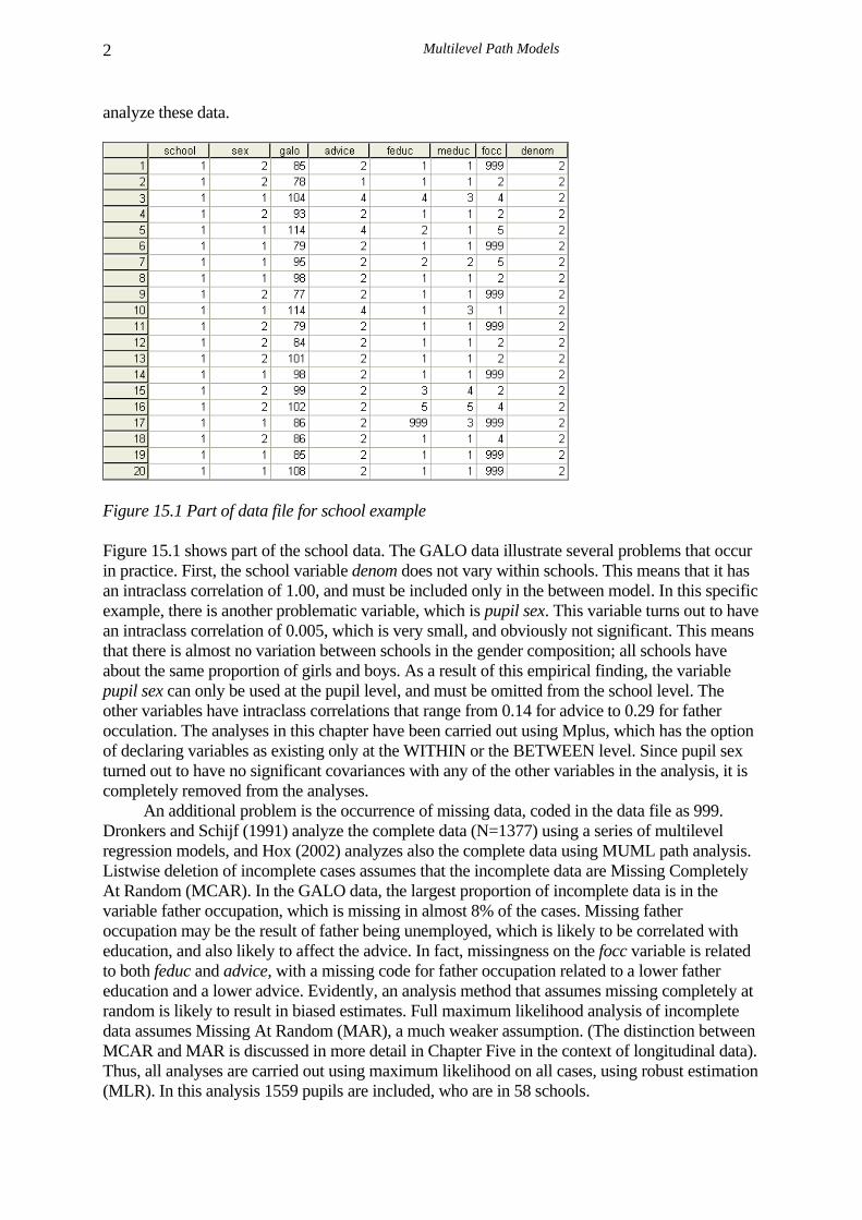
Multilevel Path Models
2
analyze these data.
Figure 15.1 Part of data file for school example Figure 15.1 shows part of the school data. The GALO data illustrate several problems that occur in practice. First, the school variable denom does not vary within schools. This means that it has an intraclass correlation of 1.00, and must be included only in the between model. In this specific example, there is another problematic variable, which is pupil sex. This variable turns out to have an intraclass correlation of 0.005, which is very small, and obviously not significant. This means that there is almost no variation between schools in the gender composition; all schools have about the same proportion of girls and boys. As a result of this empirical finding, the variable pupil sex can only be used at the pupil level, and must be omitted from the school level. The other variables have intraclass correlations that range from 0.14 for advice to 0.29 for father occulation. The analyses in this chapter have been carried out using Mplus, which has the option of declaring variables as existing only at the WITHIN or the BETWEEN level. Since pupil sex turned out to have no significant covariances with any of the other variables in the analysis, it is completely removed from the analyses. An additional problem is the occurrence of missing data, coded in the data file as 999. Dronkers and Schijf (1991) analyze the complete data (N=1377) using a series of multilevel regression models, and Hox (2002) analyzes also the complete data using MUML path analysis. Listwise deletion of incomplete cases assumes that the incomplete data are Missing Completely At Random (MCAR). In the GALO data, the largest proportion of incomplete data is in the variable father occupation, which is missing in almost 8% of the cases. Missing father occupation may be the result of father being unemployed, which is likely to be correlated with education, and also likely to affect the advice. In fact, missingness on the focc variable is related to both feduc and advice, with a missing code for father occupation related to a lower father education and a lower advice. Evidently, an analysis method that assumes missing completely at random is likely to result in biased estimates. Full maximum likelihood analysis of incomplete data assumes Missing At Random (MAR), a much weaker assumption. (The distinction between MCAR and MAR is discussed in more detail in Chapter Five in the context of longitudinal data). Thus, all analyses are carried out using maximum likelihood on all cases, using robust estimation (MLR). In this analysis 1559 pupils are included, who are in 58 schools.
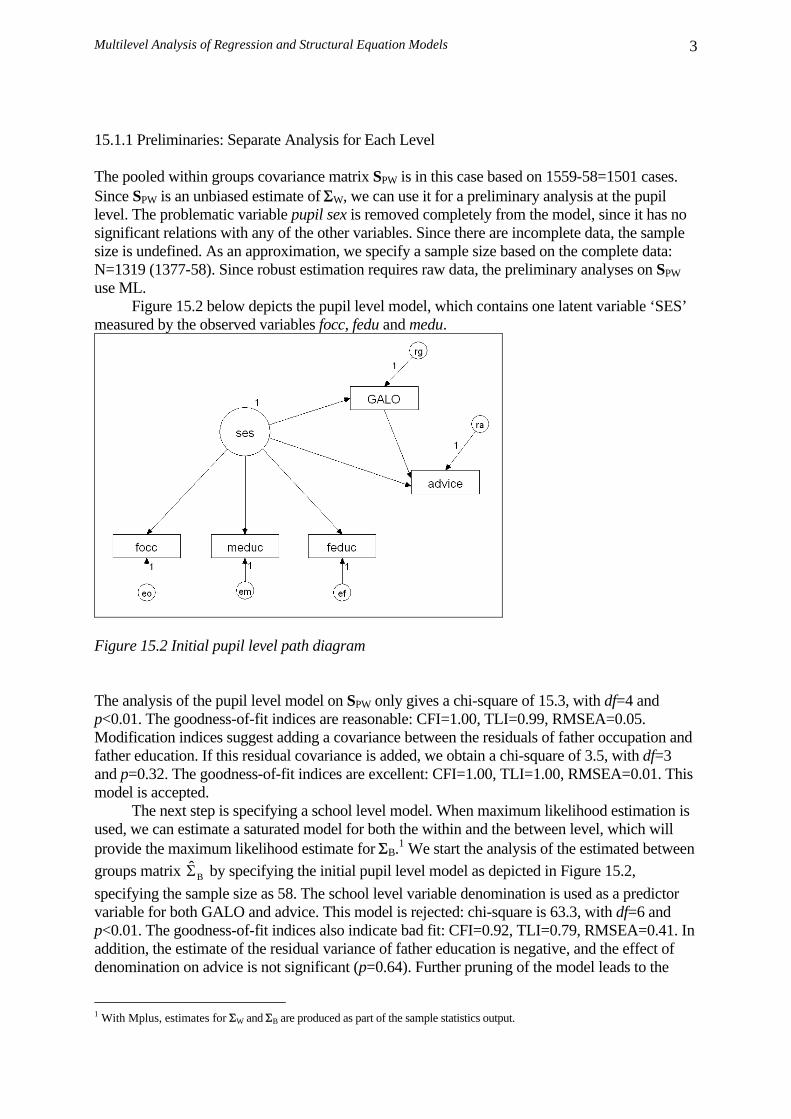
Multilevel Analysis of Regression and Structural Equation Models 3
15.1.1 Preliminaries: Separate Analysis for Each Level The pooled within groups covariance matrix SPW is in this case based on 1559-58=1501 cases. Since SPW is an unbiased estimate of ΣW, we can use it for a preliminary analysis at the pupil level. The problematic variable pupil sex is removed completely from the model, since it has no significant relations with any of the other variables. Since there are incomplete data, the sample size is undefined. As an approximation, we specify a sample size based on the complete data: N=1319 (1377-58). Since robust estimation requires raw data, the preliminary analyses on SPW use ML. Figure 15.2 below depicts the pupil level model, which contains one latent variable ‘SES’ measured by the observed variables focc, fedu and medu.
Figure 15.2 Initial pupil level path diagram The analysis of the pupil level model on SPW only gives a chi-square of 15.3, with df=4 and p<0.01. The goodness-of-fit indices are reasonable: CFI=1.00, TLI=0.99, RMSEA=0.05. Modification indices suggest adding a covariance between the residuals of father occupation and father education. If this residual covariance is added, we obtain a chi-square of 3.5, with df=3 and p=0.32. The goodness-of-fit indices are excellent: CFI=1.00, TLI=1.00, RMSEA=0.01. This model is accepted.
The next step is specifying a school level model. When maximum likelihood estimation is used, we can estimate a saturated model for both the within and the between level, which will provide the maximum likelihood estimate for ΣB.1 We start the analysis of the estimated between groups matrix BΣ by specifying the initial pupil level model as depicted in Figure 15.2, specifying the sample size as 58. The school level variable denomination is used as a predictor variable for both GALO and advice. This model is rejected: chi-square is 63.3, with df=6 and p<0.01. The goodness-of-fit indices also indicate bad fit: CFI=0.92, TLI=0.79, RMSEA=0.41. In addition, the estimate of the residual variance of father education is negative, and the effect of denomination on advice is not significant (p=0.64). Further pruning of the model leads to the
1 With Mplus, estimates for ΣW and ΣB are produced as part of the sample statistics output.

Multilevel Path Models
4
model depicted in Figure 15.4. This model still does not fit well: chi-square is 65.6, with df=8 and p<0.01. The goodness-of-fit indices also indicate bad fit: CFI=0.92, TLI=0.84, RMSEA=0.35. There are no large modification indices, so there are no obvious ways to improve the school level model.
Figure 15.4 Final school level path diagram, SES as latent variable Observation of the school level correlation matrix shows that at the school level father education and mother education have a high correlation, while the correlations with father occupation are much lower. Also, the covariances of father occupation and father education with other variables appear different. This indicates that assuming a latent variable SES at the school level may be wrong. An entirely different way to model the effect of these variables on GALO and advice is to use a model with only observed variables. The initial path diagram for such a model is in Figure 15.5.
Figure 15.5 Initial school level path diagram, regression model The model depicted in Figure 15.5 is a saturated model, and therefore cannot fail to fit. It turns out that the effects of denomination and father occupation on advice are not significant, so the

Multilevel Analysis of Regression and Structural Equation Models 5
final model becomes:
Figure 15.6 Final school level path diagram, regression model The final school level model fits well: chi-square is 2.1, with df=2 and p=0.34. The goodness-of-fit indices also indicate good fit: CFI/TLI=1.00, RMSEA=0.04. The SES model in Figure 15.4 and the regression model in Figure 15.6 are not nested, but they can be compared using the information criteria AIC and BIC. For the SES model AIC=148.03 and BIC=172.76, and for the regression model AIC=78.56 and BIC=97.11. Both the AIC and the BIC indicate a preference for the regression model. 15.1.2 Putting It Together: Two-Level Analysis The preliminary analyses give a good indication of what to expect when the models are combined in a two-level model, with simultaneous estimation on both levels. There will be differences. Firstly, because the two-level analysis is simultaneous, misspecifications on one level will also affect the other level. This has a positive side as well. The estimated between groups covariance matrix used earlier is estimated using a saturated model for the within groups part. If we have a well-fitting parsimonious within model, the between model is more stable. Secondly, the preliminary analyses are based on maximum likelihood estimates of the corresponding population covariances, but in the presence of incomplete data the sample size is an approximation. When the individual level model is combined with a school level model in a simultaneous analysis, it turns out that the model with latent variable SES at the school level fits better than the model with regressions on observed variables only. Table 15.1 presents the chi-squares and fit indices for several different school level models, all fitted with the within schools model established earlier, and the fit indices CFI, TLI and RMSEA calculated by hand specifically for the school level. Table 15.1 Fit indices for several school level models Model: χ2 df p CFI TLI RMSE
A AIC*
BIC*
Indep. 577.7
18 .00 – – – 5560
5684
SES 11.0 11 .45 1.00 1.00 .00 5124
5279
Regres 22.9 8 .00 .97 .94 .03 514 531
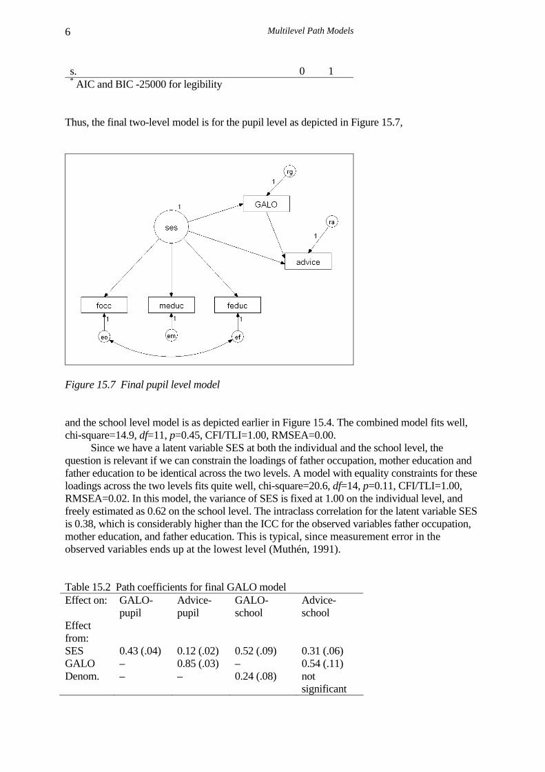
Multilevel Path Models
6
s. 0 1 * AIC and BIC -25000 for legibility
Thus, the final two-level model is for the pupil level as depicted in Figure 15.7,
Figure 15.7 Final pupil level model and the school level model is as depicted earlier in Figure 15.4. The combined model fits well, chi-square=14.9, df=11, p=0.45, CFI/TLI=1.00, RMSEA=0.00. Since we have a latent variable SES at both the individual and the school level, the question is relevant if we can constrain the loadings of father occupation, mother education and father education to be identical across the two levels. A model with equality constraints for these loadings across the two levels fits quite well, chi-square=20.6, df=14, p=0.11, CFI/TLI=1.00, RMSEA=0.02. In this model, the variance of SES is fixed at 1.00 on the individual level, and freely estimated as 0.62 on the school level. The intraclass correlation for the latent variable SES is 0.38, which is considerably higher than the ICC for the observed variables father occupation, mother education, and father education. This is typical, since measurement error in the observed variables ends up at the lowest level (Muthén, 1991). Table 15.2 Path coefficients for final GALO model Effect on: GALO-
pupil Advice-pupil
GALO-school
Advice-school
Effect from:
SES 0.43 (.04) 0.12 (.02) 0.52 (.09) 0.31 (.06) GALO – 0.85 (.03) – 0.54 (.11) Denom. – – 0.24 (.08) not
significant

Multilevel Analysis of Regression and Structural Equation Models 7
Table 15.2 presents the path coefficients and corresponding standard errors. There are strong school level effects on the GALO score and on the advice. The school level variable denomination turns out to have an effect only on the school level GALO test score. In the multilevel regression analyses presented by Schijf and Dronkers (1991), denomination has a significant effect on both the teachers’ advice and on the GALO tests score. The path model presented here shows that the main influence is through the GALO test score; the different advices given by teachers in schools of different denominations are apparently the result of differences in GALO test scores between such schools. This is precisely the kind of result that a sequence of separate regression analyses cannot show. Figure 15.4 also shows that SES has a school level effect on the variables GALO and advice. The interpretation is not that some schools simply happen to have more high SES pupils and therefore perform better; sampling differences between schools in SES composition are accounted for in the pupil model that is also fitted for the school level covariances. Instead, the substantive interpretation of the school level results must be in terms of some kind of contextual or systematic selection effect. It appears that the concentration of high or low SES pupils has its own effect on the school career variables. It is interesting to note that, on the school level, the effect of the school average on the GALO test on the average advice is negative. This can be interpreted as a typical context effect, in which the GALO score is apparently interpreted differently by teachers if the overall score of a school on the test is high. On individual level the effect of SES on the advice is partially channeled via the GALO score, and on the school level the effect of SES is partially channeled via GALO, and the effect of . Table 15.3 presents the 15.2 STATISTICAL AND SOFTWARE ISSUES IN MULTILEVEL FACTOR AND PATH MODELS It should be noted that multilevel factor and path models differ from multilevel regression models, because in general they do not have random regression slopes. The variation and covariation on the group level is intercept variation. There are also in general no cross-level and interaction effects. In multilevel factor models, the group level variation can properly be interpreted as group level variance of the group means of the latent factors. In path analysis, the interpretation of group level path coefficients is in terms of contextual effects, which are added to the individual effects. Inclusion of cross-level and other interaction terms in structural equation models is possible, but they are difficult to specify and estimate in most current SEM software (cf. Jöreskog & Yang, 1996; Schumacker & Marcoulides, 1998; Marcoulides & Schumacker, 2001). The two step direct estimation approach does not require special software. The Muthén pseudobalanced approach can be applied in any SEM software that supports multiple group analysis. Both Muthén’s pseudobalanced approach and direct estimation of the within and between covariance matrices have strong limitations. Direct estimation of the covariance matrices, followed by standard SEM analyses, ignores the fact that these covariances are themselves estimates, and that with incomplete data it is misleading to assign a single sample size to each matrix. The pseudobalanced approach, although consistent, is not very accurate. As discussed in the chapter on multilevel CFA, both simulation studies (Hox and Maas, 2001a; Hox, Maas & Brinkuis, 2008) and analytical work (Yuan and Hayashi, 2005) show that the degree of inaccuracy depends on the degree of unbalance, and that larger sample sizes do not improve the accuracy with unbalanced data.

Multilevel Path Models
8
Raudenbush and Sampson (1999b) advocate a different method to analyze multilevel models with latent variables, using standard multilevel regression software. They represent measurement error in a separate ‘variables’ level (Raudenbush, Rowan & Kang, 1991), a method described in the multivariate multilevel measurement models section in Chapter Ten of this book. The random regression coefficients at the second level are interpreted as latent variables or factors, indicated by the variables to which they are linked by sets of dummy variables. Using the means and covariances at the higher levels, path coefficients can be estimated with the corresponding standard errors. This approach, incorporated in the software HLM, can be used to estimate both factor and path models. The major advantages of their approach are that it can include random regression coefficients, and it works fine with incomplete data, which are difficult to handle in the pseudobalanced approach. The major disadvantage is the simplicity of the measurement model. The model requires that all the factor loadings are known; typically they are all set equal to one. This is a strong assumption, which implies that all observed variables that load on the same factor are measured on the same scale and have the same error variance. There are also no fit indices, so information on how well the factor or path model fits is not readily available. A full Maximum Likelihood solution to the problem of multilevel factor and path analysis requires maximization of a complicated likelihood function. Bentler & Liang (2001) describe a method to maximize the multilevel likelihood for both confirmatory factor and path models, which is implemented in the software EQS. LISREL (8.5 and later; du Toit & du Toit, 2001) includes a full maximum likelihood estimation procedure for multilevel confirmatory factor and path models, including an option to analyze incomplete data. The LISREL 8.5 user’s manual (du Toit & du Toit, 2001) cautions that this procedure still has some problems; it frequently encounters convergence problems, and needs good starting values. Mplus (Muthén & Muthén, 1998-2007) includes several options for multilevel factor and path analysis. In addition to the pseudobalanced Muml approach, Mplus offers weighted least squares and full maximum likelihood estimation. Mplus allows fitting multilevel structural equation models with random coefficients, regressions among latent variables varying at two different levels, and mixtures of continuous and ordered or dichotomous data. Rabe-Hesketh et al. (Rabe-Hesketh, Pickles & Taylor, 2000; Rabe-Hesketh & Skrondal, 2008) describe a very general software called GLLAMM (for Generalized Linear Latent And Mixed Models) that runs in the statistical package STATA (Statacorp, 2001). The program and manual are available for free (Rabe-Hesketh, Skrondal & Pickles, 2004), but the commercial package STATA is needed to run it. Like Mplus, GLLAMM can fit very general multilevel structural equation models, with no formal limit to the number of levels. Many more complex types of multilevel path models with latent variables, for instance including random slopes and cross-level effects, can be estimated using Bayesian methods. Bayesian models for continuous data are described by Goldstein and Browne (2001) and Jedidi and Ansari (2001), and models for binary data by Ansari and Jedidi (2000). Many multilevel structural equation models can be estimated using Bayesian methods and the software BUGS (Spiegelhalter, 1994), but this requires an intimate knowledge of both structural equation modeling and Bayesian estimation methods. The software REALCOM (multilevel modeling for realistically complex data; Goldstein, Steele, Rasbash & Charlton, 2007) also includes Bayesian methods for complex multilevel modeling. It is clear that there are many developments in multilevel factor and path analysis, but most require sophisticated and detailed statistical knowledge. I consider them beyond the scope of this book, especially since it will take time before these methods find their way in generally available and user-friendly software packages. Given its general availability in modern SEM software, maximum likelihood estimation is the preferred method. For nonnormal data, weighted least squares is attractive because it is computationally faster, but this is available only in Mplus.

Multilevel Analysis of Regression and Structural Equation Models 9
The analysis issues in multilevel path models, whether analyzed using Muthén’s pseudobalanced approach, using directly estimated within and between groups covariance matrices, or full maximum likelihood estimation, are comparable to the issues in multilevel factor analysis. Thus, the recommendations given in Chapter Fourteen about inspecting goodness-of-fit indices separately for the distinct levels that exist in the data, and about the separate standardization, also apply to multilevel path models. All approaches to multilevel factor and path analysis model only one single within groups covariance matrix. In doing so, they commonly assume that the within groups covariances are homogeneous, i.e., that all groups have the same within groups covariance matrix. This is not necessarily the case. The effect of violating this assumption is currently unknown. Simulation studies on the assumption of homogeneous covariance matrices in MANOVA show that MANOVA is robust against moderate differences in the covariances, provided the group sizes are not too different (Stevens, 2009). Strongly different group sizes pose a problem in MANOVA. When larger variability exists in the smaller group sizes, the between group variation is overestimated; when larger variability exists in the larger group sizes, the between group variation is underestimated. If we assume that the covariance matrices differ in different groups, one possible solution is to divide the groups in two or more separate subsets, with each subset having its own within groups model. For instance, we may assume that within group covariances differ for male and female respondents. Or, in the situation where we have larger variances in small groups and vice versa, we may divide the data into a set of small and a set of large groups. Then we model a different within groups model for each set of groups, and a common between groups model. Mplus and GLLAMM allow latent groups, which is a different way to allow different covariance matrices at the individual or the group level. APPENDIX This global variable denomination does not exist on the individual level. If we disaggregate denomination to the individual level, we will find that this disaggregated variable is constant within each school, and that the variance and all the covariances with the other individual deviation scores are zero. In software that requires the same number of variables in both groups, this problem is solved by viewing the school level variable denomination as a variable that is systematically missing in the pupil level data. The trick is that the variable denomination is included in the (school level) scaled between schools covariance matrix in the usual way. In the (pupil level) pooled within schools covariance matrix, we include denomination as a variable with a variance equal to one and all covariances with other variables equal to zero. In the within school models, there are no paths pointing to or from this observed variable. Subsequently, we fix for this variable the residual error variance to 1.00. Since this produces a perfect fit for this ‘ghost’ variable, inclusion of this variable has no influence on the within school estimates or the overall chi-square. There is only one problem; a program like LISREL assumes that this variable represents a real observed variable, and will include it when it enumerates the degrees of freedom for the within schools model. As a result, the df and therefore the p-values (and most fit-indices) in the LISREL output are incorrect, and must be corrected by hand (cf. Jöreskog & Sörbom, 1989). The df is corrected by subtracting the number of zero-covariances from the df calculated by the program. Again, some software can handle models with different numbers of observed variables in the various groups, which makes this kind of modeling much simpler.

Multilevel Path Models
10
Figure 15.8 Including a school level variable at the within-level Figure 15.8 shows how a school level variable like denom is handled in a program like Lisrel using MUML. It is included in the pooled within groups covariance matrix as a virtual variable with a variance of one, and the covariances with the other variables all set to zero. In the pupil level model, which is the model for the pooled within groups covariance matrix, the observed variable denom is modeled as independent from all other variables in the model, with an error term ed that has a variance fixed at 1. This of course exactly models the variance of one and the covariances of zero that were added to the pooled within groups covariance matrix. The problem is that a program like LISREL counts an extra variance plus five covariances in the input matrix, which means that it counts an extra six degrees of freedom. Since these nonexistent variance and covariances are necessarily estimated perfectly, the fit of the model appears spuriously good. For this reason, the degrees of freedom df must be corrected by subtracting 6, and the p-value and all goodness-of-fit indices that depend on the degrees of freedom must also be corrected.