1 Introduction to Cosmology and String Theory - … · 4 1 Introduction to Cosmology and String...

1

1Introduction to Cosmology and String TheoryJohanna Erdmenger and Martin Ammon

1.1Introduction

Cosmology and string theory are two areas of fundamental physics which haveprogressed significantly over the last 25 years. Joining both areas together providesthe possibility of finding microscopic explanations for the history of the early uni-verse on the one hand, and of deriving observational tests for string theory on theother. In the subsequent seven chapters, different aspects of string cosmology areintroduced and discussed.

This chapter contains a summary of the basics of both cosmology and stringtheory in view of providing a reference and glossary for the subsequent chapters.The basic concepts are introduced and briefly described, emphasizing those aspectswhich are used in the remainder of this book.

There is a wealth of excellent textbooks of both cosmology and string theory,to which readers interested in further details are referred to – for example [1–7].Reviews on string cosmology include [8–11]. An introduction to string cosmologyis found in the textbook [12].

Cosmology is introduced in Sections (1.2)–(1.4) below, and string theory in Sec-tions (1.5)–(1.11).

1.2Foundations of Cosmology

On the basis of experimental evidence, the common scenario of present-day cos-mology is the model of the hot big bang, according to which the universe originatedin a hot and dense initial state 13.7 billion years ago, and then has expanded and isstill expanding. The most essential feature of the present-day universe is that it ishomogeneous and isotropic, that is its structure is the same at every point and inevery direction.

This “standard model of cosmology” has received substantial experimental back-up, beginning with the discovery of the cosmic microwave background (CMB) ra-

String Cosmology. Edited by Johanna ErdmengerCopyright © 2009 WILEY-VCH Verlag GmbH & Co. KGaA, WeinheimISBN: 978-3-527-40862-7

2 1 Introduction to Cosmology and String Theory

diation by Penzias and Wilson in 1964 [13]. In recent years, a wealth of precise datahas been collected. We list just a few of the important new observations here: In the1990s, observations of galaxies with the Hubble Space Telescope led in particularto an accurate measurement of the Hubble parameter. Fluctuations in the cosmicmicrowave background radiations have been observed with the COBE satellite, andsubsequently with the BOOMERanG experiment. A further increase in precisioncame with the WMAP satellite launched in 2001, whose measurements of the pa-rameters of the standard model of cosmology are consistent with the conclusionthat the present-day universe is flat. Moreover, these measurements support thescenario of cosmic inflation. They will be supplemented by further data from thePLANCK satellite in the near future.

1.2.1Metric and Einstein Equations

The homogeneity and isotropy of the universe is best described by the Robertson–Walker metric, which in (–, +, +, +) signature commonly used in string theory reads

ds2 = –dt2 + a2(t)»

dr 2

1 – κr+ r 2(dθ2 + sin2 θdφ2)

–. (1.1)

Here a(t) describes the relative size of space-like hypersurfaces at different times.κ = +1, 0, –1 stands for positively curved, flat, and negatively curved hypersurfaces,respectively. The frequency of a photon traveling through the expanding universeexperiences a redshift z of the size

1 + z =λobserved

λemitted=

apresent

aemitted, (1.2)

where λ denotes the photon wavelength.Using the scale factor a(t) we define the Hubble parameter

H ==aa

, (1.3)

with a(t) = da/dt. As was first discovered and suggested by Edwin Hubble, andhas been verified with high precision by modern observational methods, the mostdistant galaxies recede from us with a velocity given by the Hubble law,

v � Hd , (1.4)

where d is the distance between us and the galaxies considered.For describing the expanding universe it is often useful to use the term e-foldings,

defined as e == ln(a(tf)/a(ti)), which describes the growth of the scale factor betweensome time ti and a later time tf.

The dynamics governing the evolution of the scale factor a(t) are obtained frominserting the Robertson–Walker metric into the Einstein equation

Rμν –12

R g μν = 8πGTμν , (1.5)

1.2 Foundations of Cosmology 3

where Rμν and R are the Ricci tensor and scalar, G the Newton constant, and Tμν

the energy–momentum tensor. The universe is best described by the perfect fluidform for the energy–momentum tensor of cosmological matter, given by

Tμν = (ρ + p)uμuν + pg μν , (1.6)

where uμ is the fluid four-velocity, ρ is the energy density in the rest frame of thefluid, and p is the pressure in the same frame. For consistency with the Robertson–Walker metric, fluid elements are comoving in the cosmological rest frame, withnormalized four-velocity

uμ = (1, 0, 0, 0) . (1.7)

The energy–momentum tensor is diagonal and takes the form

Tμν =

ρ

pgij

!, (1.8)

where gij stands for the spatial part of the Robertson–Walker metric, including thefactor of a2(t). Inserting the Robertson–Walker metric (1.1) into the Einstein equa-tion (1.5) with the energy–momentum tensor (1.6), we obtain the first Friedmannequation

H2 ==„

aa

«2

=8πG

3

Xj

ρj –κ

a2 , (1.9)

with the total energy density ρ =P

j ρj, where the sum is over all different types ofenergy density in the universe. Moreover, we have the evolution equation

aa

+12

„aa

«2

= –4πGX

j

pj –κ

2a2 . (1.10)

Here pj labels the different types of momenta. Equations (1.9) and (1.10) may becombined into the second Friedmann equation

aa

= –4πG

3

Xj

`ρj + 3pj

´. (1.11)

The first Friedmann equation may be used to define the critical energy density

ρc ==

0@X

j

ρj

1A

c

=3H2

8πG� 10–29 g

cm3 , (1.12)

for which κ = 0 and space is flat. The density ratio

Ωtotal ==ρρc

(1.13)


thus allows us to relate the total energy density of the universe to its curvaturebehavior,

Ωtotal > 1 ⇔ κ = 1 ,Ωtotal = 1 ⇔ κ = 0 ,Ωtotal < 1 ⇔ κ = –1 .

(1.14)

Recent WMAP observations have shown that today, Ωtotal = 1 to great accuracy,which leads to the conclusion that the universe is flat.

Energy conservation, ∇μTμν = 0, gives the relation

ρ + 3H(ρ + p) = 0 . (1.15)

This relation is not independent of the Friedmann equations. Using both of them,energy conservation (1.15) may be rewritten as

ddt`ρa3´ = –p

ddt

a3 . (1.16)

1.2.2Energy Content of the Universe

There is good experimental evidence, in particular from WMAP measurements,that the cosmic fluid contains four different components, and that the total energydensity ρtotal in the universe is equal to the critical density ρc given by (1.12). Thisimplies

Ωtotal =X

j

Ωj = 1 , Ωj =ρj

ρc, (1.17)

with Ωj denoting the present-day fraction of the energy density contributed by thej-th fluid component. The four components of the cosmic fluid are the following:1. Radiation: this component contains predominantly photons, most of which cor-respond to the cosmic microwave background. The photons are thermally distrib-uted with temperature T = 2.715 K. The gas of photons satisfies the equation ofstate

pRad =13

ρRad . (1.18)

Moreover, there are also cosmic relic neutrinos in this fluid component, thermallydistributed with T = 1.9 K. The total energy density of radiation is a small fraction,

ΩRad W 8 ~10–5 , (1.19)

of the total present-day energy density.2. Baryons: since their rest mass is much larger than their kinetic energy, theirequation of state is

pB � 0 . (1.20)

1.2 Foundations of Cosmology 5

Their energy fraction is

ΩB W 4% . (1.21)

3. Dark Matter: observations of galaxy movement and of matter influence on fluctu-ations in the CMB provide evidence that there has to be a large amount of long-livednonrelativistic matter subject to gravitation, which is not detectable by its emittedradiation. Determining the exact structure of this dark matter remains one of theessential challenges of modern cosmology. Just as for the baryons, dark matter hasthe equation of state

pDM � 0 , (1.22)

while its energy fraction is

ΩDM W 26% , (1.23)

so that the overall density of nonrelativistic matter is

ΩM == ΩB + ΩDM W 30% . (1.24)

4. Dark Energy: a fourth, similarly unexplained contribution to the cosmic fluid isdark energy, which for a total energy density Ω = 1, has to be present in the universewith the large fraction

ΩDE W 70% . (1.25)

Its equation of state is expected to be

pDE = –ρDE . (1.26)

Observational evidence that such a fluid component with negative pressure mustbe present include tests of the Hubble expansion rate using supernovae whichimply that the overall expansion rate of the universe, the Hubble parameter H =a/a, is increasing at present. The Friedmann equation (1.11) implies that this canonly happen for positive energy density if the total pressure is sufficiently negative,p < –1/3ρ. Since none of the other fluid components has negative pressure, a largefraction of such a component must be present.

Each of the above equations of state implies that wj = pj/ρj is time independent,with

wRad =13

, wM = 0 , wDE = –1 . (1.27)

Inserting these values into the energy conservation condition in the form (1.16) weobtain, with a0 the present-day value of a,

ρj = ρj,0

“a0

a

”αj

, αj = 3(1 + wj) , (1.28)


where

αRad = 4 , αM = 3 , αDE = 0 . (1.29)

The different equations of state for the different fluid components thus imply thattheir relative abundances differ in the past universe as compared to the present-dayobservations since their energy densities vary differently as the universe expands.The history of the universe splits into periods where radiation, matter, and darkenergy dominate the evolution of the total density, consecutively. The transition be-tween the radiation and matter-dominated regimes is called radiation–matter equali-ty and occurs at a scale given by the comoving wave vector of magnitude k � (aH)eq.Note also that the Friedmann equation (1.9) implies that for w > –1/3, the scale fac-tor a(t) grows more slowly than the Hubble scale H–1(t).

It is useful to define the comoving frame which moves along with the Hubble flow.A comoving observer is the only one which sees an isotropic universe.

1.2.3Development of the Universe

During its expansion the universe experienced a number of decisive physicalevents. The earliest cosmological event for which there is observational evidenceis nucleosynthesis, which began about three minutes after the big bang, and lastedfor about fifteen minutes. At this time, the universe cooled below 1 MeV and lightnuclei, hydrogen, helium, lithium, and beryllium, began to accumulate from pro-tons and neutrons. The observational evidence for nucleosynthesis comes frommeasuring the relative abundance of these elements.

The radiation–matter crossover described above occurred at a redshift (1.2) of z ~3600, or about 50 000 years after the big bang. After this crossover, density inho-mogeneities can grow only logarithmically with a while they grow linearly with aduring radiation domination.

At a redshift of around z ~ 1100, or about 380 000 years after the big bang,recombination of nuclei and electrons into electrically neutral atoms occurs. Thisis the origin of the cosmic microwave background which corresponds to the lightwhich is free to move through the universe after recombination. Beforehand, pho-tons interact with the charged medium surrounding them on short scales. TheCMB corresponds to a surface of last scattering for the photons. Measurementsof the CMB temperature fluctuations, which are of the order δT/T ~ 10–5, pro-vide direct information about the size of primordial density fluctuations at thistime.

Finally, galaxy formation occurs in the universe once the primordial density fluc-tuations have been amplified to a scale at which they are no longer well-describedby linear perturbations. According to the cold dark matter model (for reviews seefor instance [14]), the distribution of galaxies observed today also requires thepresence of nonrelativistic (cold) dark matter, together with nonlinear fluctua-tions.

1.3 Inflation 7

1.3Inflation

1.3.1Puzzles Within the Big Bang Model

When considering the initial conditions characterizing matter in the big bang sce-nario of an expanding universe, we encounter a number of puzzles. Three of themare discussed in the subsequent text. The initial conditions fix the matter distrib-ution in the universe at the Planckian time of tp = 10–43 s when classical gravitybecomes applicable.

Horizon problem. The horizon problem relates to the fact that the universe is soextremely homogeneous. The Friedmann equation (1.9) implies that the universeexpands so quickly that thermal equilibration would violate causality. A dimension-al analysis for the ratio ai/a0 of the initial and the present-day value of the scale fac-tor a(t) shows that our universe was initially larger than a casual patch by a factor ofthe order ai/a0. If expansion was always decelerated by an attractive gravity force,which implies ai/a0 >> 1, then the homogeneity scale was always larger than thecausality scale. In fact, using the present size of the universe, the Planck time andthe temperature of the universe now and at Planck time, one finds that ai/a0 ~ 1028.This would require an extraordinary fine tuning.

Flatness problem. While the horizon problem relates to the initial conditions forthe spatial distribution of matter, the flatness problem relates to the initial veloci-ties. These must satisfy the Hubble law (1.4). The ratio of the kinetic to the totalenergy of matter in the universe is again given by (ai/a0)2 and if this ratio is verylarge, a very unnatural fine tuning between the kinetic energy associated to Hub-ble expansion and the gravitational potential energy is required. This may be seenfrom the Friedmann equation (1.9) which implies

Ω(t) – 1 =κ

(Ha)2 , (1.30)

and thus, since the present-day Ω0 has been observed to be very close to unity,

Ωi – 1 = (Ω0 – 1)„

a0

ai

«2

< 10–56 (1.31)

for ai/a0 ~ 1028. Such an astonishing fine-tuning appears implausible.Initial perturbations. A third puzzle, related to the other two, concerns the origin

of the original inhomogeneities needed to explain the large-scale structure of thepresent-day universe.

1.3.2The Concept of Inflation

A concept which can solve the puzzles mentioned is inflation. The idea of inflation,first suggested in [15], is that there is an initial stage of accelerated expansion where


gravity acts as a repulsive force. If gravity was always positive, then ai/a0 is neces-sarily larger than one since gravity decelerates expansion. ai/a0 < 1 is possible onlyif gravity is repulsive during some period of expansion. This period of repulsivegravity can in particular explain the creation of our universe from a single causallyconnected region. Moreover, since it accelerates expansion, small initial velocitiesinside a causally connected region become very large.

In the inflationary period we have a > 0. From the Friedmann equation (1.11),which may be written in the form

a = –4πG

3(ρ + 3p)a , (1.32)

for the total energy density ρ and the total momentum p. We read off that a > 0requires ρ + 3p < 0. This implies that the strong energy dominance condition,ρ + 3p > 0, must be violated during inflation. One example which violates thiscondition is a positive cosmological constant for which p W –ρ.

Inflation can only appear during a limited period in time for consistency withcosmological observations. In simple inflationary models it takes place in the peri-od of tinf ~ 10–36 – 10–34 s after the big bang. It must end with a “graceful exit”, afterwhich a becomes negative again.

Let us consider how the condition p = –ρ may be realized. The matter and itsinteractions during inflation is simply modeled by a single scalar field ϕ = ϕ(t), theinflaton. This can be viewed as an order parameter describing the vacuum of thephysical theory determining the very high energy physics. This gives rise to

ρ =12ϕ2 + V(ϕ) , p =

12ϕ2 – V(ϕ) , (1.33)

with potential V(ϕ). The condition p W –ρ requires ϕ2 << V(ϕ), so the kinetic energymust be smaller than the potential energy. This is referred to as “slow roll”. TheKlein–Gordon equation or ρ = –3H(ρ + p) imply

ϕ + 3Hϕ + V ′ = 0 , V ′ ==∂V∂ϕ

. (1.34)

The second term in this equation corresponds to a friction term proportional to H.Generically if friction becomes large, we may neglect the second derivative term ϕ

and find an approximate asymptotic solution to (1.34). With ϕ = 0, (1.34) implies

ϕ W –„

V ′

3H

«. (1.35)

From the slow-roll condition 1/2ϕ2 << V we then obtain the two conditions

ε << 1, η << 1 (1.36)

for the slow-roll parameters

ε ==12

„MpV ′

V

«2

, η ==M2

pV ′′

V. (1.37)

1.4 Fluctuations 9

Single-field slow-roll inflation leads to important consequences for density fluctua-tions, as discussed in Section 1.4.3 below, and in further detail in Chapters 2 and 3.It turns out that these consequences can be described just in terms of the twosmall parameters ε and η, together with the value of the Hubble parameter duringinflation.

1.4Fluctuations

1.4.1Characterization of Small Fluctuations

An important question of cosmology is to study how the large-scale structure of theuniverse which is observed today, including galaxies and clusters of galaxies, devel-oped from the initially flat and homogeneous universe. The large-scale structurehas evolved from initially small fluctuations during the expansion of the universe.These small fluctuations are taken as initial conditions of the big bang model.

In linear approximation, the fluctuations of the Robertson–Walker metric (1.1),given by

ds2 =ˆ(0)g μν + δg μν(x)

˜dx μ dxν , (1.38)

may be decomposed as follows using the symmetry properties of the unperturbedRobertson–Walker metric. The linear approximation applies to fluctuations onlength scales below the Hubble scale. It implies that the different fluctuationmodes decouple and have a Gaussian distribution.

The δg00 component has the form

δg00 = 2a2φ , (1.39)

with scalar φ. The spacetime component δg0i has the form

δg0i = a2(∂iB + Si) , (1.40)

where the index i runs over the three space-like components. The vector Si satisfies∂iSi = 0. The fluctuation component δgij is a tensor under 3-rotations and may bewritten as

δgij = a2(2ψδij + 2∂i∂jE + ∂iFj + ∂jFi + hij) , (1.41)

where ψ, E are scalars, ∂iFi = 0, hii = 0, ∂ihi

j = 0.The fluctuations are thus described by the scalar fluctuations φ, ψ, B, E, the vector

fluctuations Si, Fi, and the tensor fluctuations hij. The latter described gravitation-al waves. All of these functions change under coordinate reparametrizations, butmay be regrouped into coordinate invariant expressions. A particularly importantcoordinate invariant combination of scalar fluctuations is

Φ == φ –1aˆa (B – E ′)

˜′ , (1.42)


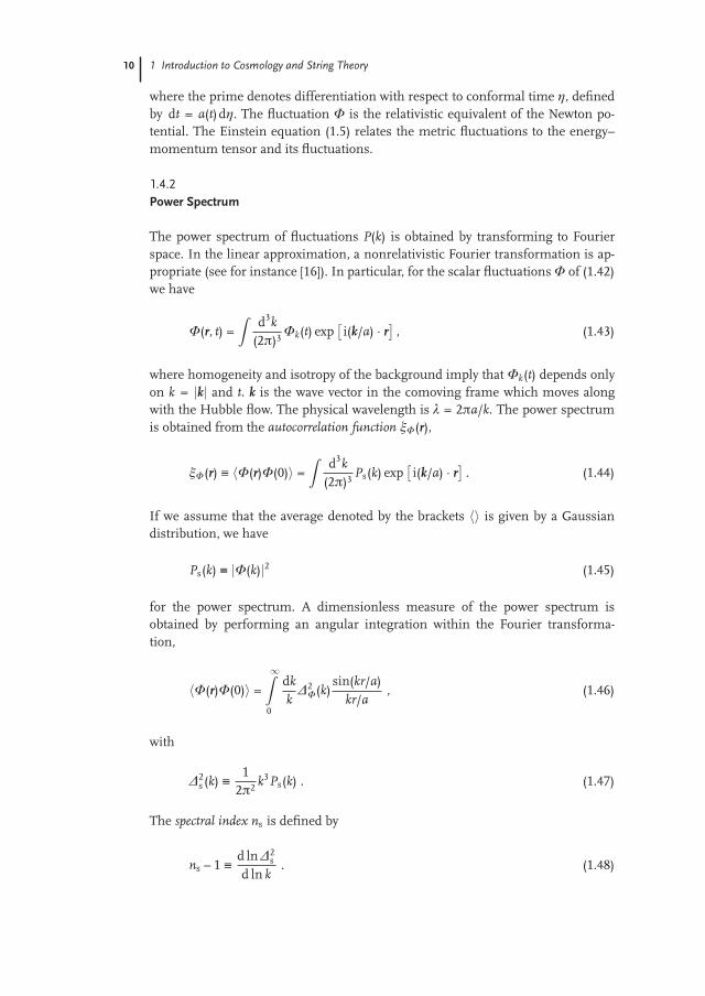
where the prime denotes differentiation with respect to conformal time η, definedby dt = a(t)dη. The fluctuation Φ is the relativistic equivalent of the Newton po-tential. The Einstein equation (1.5) relates the metric fluctuations to the energy–momentum tensor and its fluctuations.

1.4.2Power Spectrum

The power spectrum of fluctuations P(k) is obtained by transforming to Fourierspace. In the linear approximation, a nonrelativistic Fourier transformation is ap-propriate (see for instance [16]). In particular, for the scalar fluctuations Φ of (1.42)we have

Φ(r, t) =Z

d3k(2π)3 Φk(t) exp

ˆi(k/a) · r

˜, (1.43)

where homogeneity and isotropy of the background imply that Φk(t) depends onlyon k = |k| and t. k is the wave vector in the comoving frame which moves alongwith the Hubble flow. The physical wavelength is λ = 2πa/k. The power spectrumis obtained from the autocorrelation function �Φ(r),

�Φ(r) == 〈Φ(r)Φ(0)〉 =Z

d3k(2π)3 Ps(k) exp

ˆi(k/a) · r

˜. (1.44)

If we assume that the average denoted by the brackets 〈〉 is given by a Gaussiandistribution, we have

Ps(k) == |Φ(k)|2 (1.45)

for the power spectrum. A dimensionless measure of the power spectrum isobtained by performing an angular integration within the Fourier transforma-tion,

〈Φ(r)Φ(0)〉 =

∞Z0

dkk

Δ2Φ(k)

sin(kr/a)kr/a

, (1.46)

with

Δ2s (k) ==

12π2 k3Ps(k) . (1.47)

The spectral index ns is defined by

ns – 1 ==d ln Δ2

s

d ln k. (1.48)

1.4 Fluctuations 11

A spectral index of ns = 1 corresponds to a scale invariant spectrum, also calleda Harrison–Zel’dovich spectrum. For tensor fluctuations or gravitational waves,denoted by hij in (1.41), the spectral index is defined by

nT ==d ln Δ2

T

d ln k. (1.49)

These fluctuations have not yet been observed.The structure of the spectrum is influenced by the expansion of the universe.

For instance, for a spectrum which is scale invariant for modes k < keq, with keq ==(aH)eq the momentum scale at radiation–matter equality, we have a spectrum ofthe form Δ2

Φ(k) ∝ 1/k4 for modes k > keq. This behavior arises since modes withk > keq re-enter the Hubble scale before radiation–matter equivalence, while modeswith k < keq do so afterwards (remember that aH shrinks during both matter andradiation dominated periods).

1.4.3Fluctuations and Inflation

Inflation has a significant impact on the fluctuation spectrum which originatesfrom two facts. First, there are new contributions to the equations of motion forthe metric fluctuations which originate from fluctuations of the scalar inflatonfield. Second, while the scale aH shrinks during matter and radiation dominance,it grows during inflation, such that length scales L ~ a grow faster than H–1. Thereis a horizon corresponding to the graceful exit at which inflation ends, and wherethe length scales grow slower than the Hubble scale again.

In inflationary models, the fluctuations � of the inflaton φ are obtained fromlinearizing the equation of motion

qφ – V ′(φ) = 0 (1.50)

after replacing φ → φ + � and linearizing in � as well as in the metric fluctuations.The time dependence of the background forces � and the scalar metric fluctua-tion Φ to mix with each other. For instance, for k >> aH the solution for Φ of thecoupled equations shows a damped oscillation. In the opposite regime k << aH, thecoupled fluctuations equations read, in the slow-roll approximation,

3H� + V ′′(φ)� + 2V ′(φ)Φ = 0 , 2M2PHΦ = φ� . (1.51)

The solutions are, after transforming to momentum space,

�k = CkV ′(φ)V(φ)

, Φk = –Ck

2

„V ′(φ)V(φ)

«2

, (1.52)

with Ck a constant of integration. This constant is set by the initial conditions at thehorizon where the universe exits the inflation period. Since all classical fluctuations


are damped away during the inflation period, the new perturbations are fueled byquantum fluctuations. The quantization for the inflaton perturbations reads

�(x) =Z

d3k(2π)3

ˆckuk(t) exp( ik · r/a) + c∗ku∗

k(t) exp(– ik · r/a)˜

, (1.53)

where c∗k , ck are the creation and annihilation operators and uk(t) exp( ik·r/a) is a ba-sis of eigenmodes of the background field equation. Evaluating �k at the horizonexit the, where k = aH, determines the integration constant to be

Ck = uk(the)„

VV ′

«he

. (1.54)

Using this, the result for the power spectrum for the scalar metric fluctuationseventually reads

Δ2Φ(k) =

„V

24π2M4Pε

«he

, (1.55)

with ε the slow-roll parameter defined in (1.37).For the spectral index (1.48) we obtain, using that

dd ln k

= –M2P

„V ′

V

«d

dϕ(1.56)

in the slow-roll approximation,

ns – 1 = –6ε + 2η , (1.57)

with ε, η as in (1.37), where the right hand side is evaluated at horizon exit. This im-plies that ns < 1. Therefore, inflation predicts a red tilt in the scalar power spectrum,since ns < 1 means that the amplitude for smaller momentum modes is larger thanthe amplitude for larger momentum modes. Similarly, for tensor modes inflationpredicts that

Δ2T(k) =

2V3π2M4

P, (1.58)

and

nT = –2ε (1.59)

for the tensor spectral index (1.49).This concludes our brief introduction to cosmology.

1.5Bosonic String Theory

We now turn to the essentials of string theory, emphasizing aspects relevant to thesubsequent chapters. We begin by discussing bosonic string theory, after which

1.5 Bosonic String Theory 13

we focus on superstring theories and dualities between these theories. Moreover,the unification of consistent superstring theories in ten dimensions into M-theorywill be discussed. Also, there is a short introduction to D-branes and to compact-ification scenarios of string theory to four spacetime dimensions. Finally, shortintroductions to string thermodynamics and to the AdS/CFT correspondence aregiven.

Whereas in conventional quantum field theory the elementary particles arepoint-like objects, the fundamental objects in perturbative string theory are one-dimensional strings. As a string evolves in time, it sweeps out a two-dimensionalsurface in spacetime, the world-sheet of the string, which is the string counterpartof the world-line for a point particle. To parametrize the world-sheet of the string,two parameters are needed: the world-sheet time coordinate τ = σ0, which param-etrizes the world-line in the case of a point-like particle, and σ = σ1 parametrizingthe spatial extent of the string. The embedding of the world-sheet of the fundamen-tal string into the (target) spacetime is given by the functions X μ(τ, σ), which arealso referred to as the embedding functions or target spacetime string coordinates.Since the action of a point-like particle is given by the length of the world-line, thenatural generalization to the action of a string propagating through flat spacetimeis given by the area of the world-sheet,

S = –1

2πα′

Zd2σq

– det ∂αX μ∂�Xμ , (1.60)

where d2σ = dσ0 dσ1 = dτdσ. This is the Nambu–Goto action of a fundamentalstring. The determinant is taken with respect to α, � = 0, 1, where α and � labelthe world-sheet coordinates. Moreover, we use the short-hand notation ∂α = ∂/∂σα.The only free parameter appearing in this action is α′, which is related to the lengthof the string, α′ = l2s . The dimensionful prefactor T = 1/(2πα′) can be interpreted asthe string tension or the energy per length. To get rid of the square root in the actionof the fundamental string in view of quantization, an auxiliary field hα�(σ0, σ1) isintroduced, which has to satisfy the constraints given below. This gives rise to thePolyakov action,

S = –1

4πα′

Zd2σ

√–hhα�∂αX μ∂�Xμ , (1.61)

which is classically equivalent to (1.60) using the equations of motion of hα�. In(1.61), h is the determinant of the matrix hα� and hα� is the inverse matrix ofhα�, that is hα�h�γ = δα

γ . The auxiliary field hα� is called the world-sheet metric. ThePolyakov action is invariant under the following symmetries:

– Poincaré transformationsThese transformations are global symmetries of the world-sheet fields X μ ofthe form

δX μ = ΛμνX ν + a μ and δhα� = 0 , (1.62)

where Λ μν and a μ are Lorentz transformations and spacetime translations,

respectively.


– ReparametrizationsThe Polyakov action is invariant under reparametrizations since a change inthe world-sheet parametrization of the form σ α → f α(σ) = σ′α with

hα�(σ) =∂f γ

∂σα

∂f δ

∂σ� hγδ(σ′) and X ′μ(τ′, σ ′) = X μ(τ, σ) (1.63)

does not change the action.– Weyl transformations

The action is also invariant under rescalings of the world-sheet metric hα�

hα� → eω(σ,τ)hα� and δX μ = 0 . (1.64)

Since this transformation is a local symmetry of the action, the energy–momentum tensor of the field theory defined on the world-sheet is traceless,that is T a

a = 0. After quantization, Weyl Symmetry is potentially broken bya conformal anomaly. In string theory, this anomaly has to be absent, whichis only the case if the spacetime dimension of the target space is D = 26for bosonic string theory. Moreover, there are restrictions on the form of thebackground fields allowed (see Section 1.5.4).

The local symmetries may be used to choose a gauge which brings the componentsof the world-sheet metric into a simple form. In particular, the equations of motionof the action can be simplified by choosing the gauge

hα� = ηα� =

–1 00 1

!. (1.65)

In this and other conformal gauges, the equation of motion for X μ(τ, σ) is a rela-tivistic wave equation,

`∂2

τ – ∂2σ´

X μ = 0 , (1.66)

supplemented by the Virasoro constraints

∂τX μ∂σXμ = 0 , (1.67)

∂τX μ∂τXμ – ∂σX μ∂σXμ = 0 . (1.68)

These constraints are derived from the equations of motion of the auxiliary fieldhα� in the Polyakov action and have to be satisfied to ensure the equivalence of thetwo actions (1.60) and (1.61) at the classical level.

1.5.1Open and Closed Strings

By applying variational methods, it is possible to derive not only the equations ofmotion but also the possible boundary conditions for the string. There are twodifferent types of strings: open and closed strings.


1.5.1.1Closed StringsClosed strings are topologically equivalent to a circle, that is they do not have end-points. If we parametrize these strings by the parameter σ ∈ [0, 2π[, the boundaryconditions read

X μ(τ, 0) = X μ(τ, 2π), ∂σX μ(τ, 0) = ∂σX μ(τ, 2π), hα�(τ, 0) = hα�(τ, 2π) .

(1.69)

This means that the string coordinates X μ are periodic, that is the endpoints arejoined to form a closed loop. The mode expansion for the closed string is simplygiven by a pair of left and right-moving waves, which travel around the string inopposite directions,

X μ(τ, σ) = X μR(τ – σ) + X μ

L (τ + σ) . (1.70)

XR (XL) are the right (left) moving parts, respectively. The mode decompositions ofthe left and right-moving parts are given by

X μR(τ – σ) =

12

x μ0 + α′p μ

R(τ – σ) + i

rα′

2

Xn=/0

1n

α μn e–2in(τ–σ) (1.71)

and

X μL (τ + σ) =

12

x μ0 + α′p μ

L (τ + σ) + i

rα′

2

Xn=/0

1n

α μn e–2in(τ+σ) . (1.72)

x μ0 and p μ are the center-of-mass position and momentum of the string, respective-

ly. The periodicity condition requires that p μR = p μ

L , and reality of X μ requires theconditions α μ

–n = (α μn )� and α μ

–n = (α μn )�. Moreover, the center-of-mass momentum

p μ can be identified with the zero mode of the expansion by

α μ0 = α μ

0 =

rα′

2p μ . (1.73)

1.5.1.2Open StringsFor open strings, two different boundary conditions in each direction μ of thespacetime are possible, Neumann or Dirichlet boundary conditions. In the caseof Neumann boundary conditions, the component of the momentum normal tothe boundary of the world-sheet vanishes, that is

∂σXμ(τ, 0) = ∂σXμ(τ, π) = 0 . (1.74)

Note that the open string is now parametrized by σ ∈ [0, π]. The boundary condi-tion implies that there is no momentum flowing through the ends of the string.The mode decomposition of the embedding function X μ(τ, σ) is given by

X μ(τ, σ) = x μ0 + 2α′p μτ + i

√2α′Xn=/0

1n

α μn e–inτ cos(nσ) . (1.75)


Because of the Neumann boundary condition, the left and right-moving waves ofan open string are reflected into each other. As in the case of the closed string, thecenter-of-mass momentum p μ of the string can be identified with the zero modeα μ

0 of the expansion,

α μ0 =

√2α′p μ . (1.76)

If we choose Dirichlet boundary conditions along the μ direction of spacetime, theendpoints of the string are fixed, that is

X μ(τ, 0) = X μ(τ, π) = x μ0 , (1.77)

where x μ0 is a constant. The mode decomposition is then given by

X μ(τ, σ) = x μ0 +

√2α′Xn=/0

1n

α μn e–inτ sin(nσ) . (1.78)

The string coordinate X μ is real if the usual property (α μn )� = α μ

–n holds. Note thatthe zero mode α μ

0 is not present in directions where Dirichlet boundary conditionsare imposed, since the center-of-mass momentum of the string vanishes.

The modern interpretation of open-string boundary conditions is that they cor-respond to hyperplanes, so-called Dp-branes, on which open strings can end. In pspatial dimensions and in the time direction, Neumann boundary conditions areimplemented, whereas in the remaining 26 – (p + 1) dimensions Dirichlet bound-ary conditions are used. We will have a closer look at D-branes in Section 1.7.2when we discuss T-duality and in Section 1.8. For more details on D-branes see thetextbook [7].

1.5.2Quantization

The theory can be quantized by using the standard commutation relations for thefields X μ and the momentum P μ, which is conjugate to X μ. These commutationrelations imply commutation relations for creation and annihilation operators, α μ

n

and α μn , acting on the ground state of the fundamental string.1)

The masses squared M2 of the excited states are

M2 =1α′ (N – 1) (1.79)

for open strings and

M2 =2α′ (N + N – 2) (1.80)

1) We consider only noninteracting strings. Thecreation and annihilation operators can beconsidered as exciting internal degrees offreedom of the string.


for closed strings. N and N are the mass levels and are given by

N =∞X

n=1

α μ–nαn μ, N =

∞Xn=1

α μ–nαn μ . (1.81)

The mass levels N and N have integer eigenvalues, which are also called N and N,respectively.

Physical string states of the closed string have to obey the level-matching con-dition N = N for the mass levels. Because of this condition, α μ

n and α μn are not

independent. The spectrum of the closed string at the first two mass levels consistsof

– N = N = 0: tachyon with mass M2 = –4/α′.– N = N = 1: a rank-two massless tensor field, which can be decomposed into

an antisymmetric part Bμν (the Kalb–Ramond field), a symmetric tracelesspart g μν (the graviton), and the trace of the symmetric part φ (the dilaton).

Since every string theory involves closed strings, a rank-two symmetric tensor field,which will be identified with the graviton in Section 1.5.4, is necessarily incorpo-rated in string theory. Moreover, we will see that the vacuum expectation value ofφ is related to the string coupling constant. The tachyon in the closed-string spec-trum is much more severe since it may indicate an instability of the theory. Sucha tachyon will not appear in the spectrum of closed superstrings if we demand thatsupersymmetry is not explicitly broken in the embedding space.

The physical states of the open string ending on a Dp-brane at the first two masslevels are

– N = 0: A tachyon with M2 = –1/α′ appears in the spectrum. According toSen’s conjectures [17], this is related to the fact that in bosonic string theories,D-branes are unstable and will decay to radiation of closed strings.

– N = 1: A massless vector boson. This will give rise to a U(1) gauge theoryon the Dp brane. Furthermore, if p < 25 massless scalars for each directionnormal to the Dp-brane are found in the open-string spectrum.

1.5.3String Perturbation Theory: Interactions and Scattering Amplitudes

The Feynman path integral is a very natural method for describing interactions instring theory. In this approach amplitudes are given by summing over all world-sheets, weighted by the factor exp (iS/�), which connect initial and final string con-figurations, as shown in Figure 1.1 for the closed string.

For closed oriented strings, to which we restrict ourselves in this section, thesum is taken over all oriented two-dimensional world-sheets without boundaries.

Figure 1.1 Examples of world-sheets connecting initial and final string configurations.


To take open strings into account, world-sheets with boundaries have to be includ-ed. Interactions of the strings are already implicit in the sum over world-sheets.The world-sheet of a decay of one closed string into two is given in Figure 1.2.Thus, the world-sheet is similar to a Feynman diagram in which propagator linesare replaced by cylinders. A loop now corresponds to a handle of the world-sheet.An example is shown in Figure 1.3. The partition function Z , that is the integralover all (Euclidean) world-sheet metrics hα� and over all embeddings X μ(τ, σ) isgiven by, with � = 1,

Z =Z

[dX μ]ˆ

dhα�˜

exp(–S) . (1.82)

The Euclidean action S contains the usual Polyakov action Sp, supplemented bya topological term weighting the different topologies of the string world-sheet Σ,

S = Sp + λ� with � =1

4π

ZΣ

d2σ√

hR(h) , (1.83)

where R(h) is the Ricci scalar of the world-sheet metric hα�. Since � is a topologicalterm measuring the Euler number of the world-sheet, it does not contribute to theequations of motion. The factor exp(–λ�) in the path integral only affects the rela-tive weighting of different topologies. Adding a handle to any world-sheet reducesthe Euler number by two and therefore adds a factor of exp(2λ). Since the processwhich is described by adding a handle corresponds to emitting and reabsorbinga closed string, the coupling constant of a closed string is given by gclosed = exp(λ).By analogous arguments, a string coupling constant gopen of open strings can beintroduced, which is related to gclosed by

gs == gclosed = g2open = eλ . (1.84)

Figure 1.2 Joining and splitting of strings.

Figure 1.3 Comparison between Feynman diagrams of quantumfield theory and interacting string diagrams.


Figure 1.4 Four punctures on a torus. This diagram corres-ponds to Figure 1.3. The external string states (given by thefour cylinders) in Figure 1.3 can be deformed to spikes. Inthis picture the spikes are removed and are represented bythe punctures (crosses) on the torus.

In Section 1.5.4, we will see that the string coupling constant is fixed by the vacuumexpectation value of the dilaton field.

Although it is a simple idea to sum over all world-sheets bounded by given initialand final curves, it is difficult to define this sum correctly and the resulting am-plitudes are very complicated. To simplify scattering amplitudes, we take the limitwhere the string sources are at infinity. This is precisely a S-matrix element withspecified incoming and outgoing strings which are on-shell and located at infinity.Under conformal transformations, the world-sheet can be transformed to a com-pact surface with n points removed corresponding to the external string states.Such points are called punctures. By applying the path integral, the scattering am-plitude is obtained by summing over all surfaces with n punctures and by integrat-ing at these punctures against the wave functions of the external string states. Fordetailed computational techniques see for instance [18] and standard textbooks onstring theory [3–6].

1.5.4Bosonic String Theory in Background Fields

Up to now we have considered the propagation of open and closed strings inMinkowski spacetime. By coupling the fundamental string to the massless closed-string excitations (see Section 1.5.2), strings propagating through curved space-times can be described. In particular we will see that the massless closed-stringexcitation g μν – which is traceless and symmetric – can be identified with the met-ric of the target spacetime. Since the quantized string theory in curved spacetimeshould be Weyl invariant, we obtain restrictions on the target spacetime allowed:the spacetime has to satisfy the vacuum Einstein equations (at least in the lowestorder of α′). This is the goal of this section.

Now we will generalize the (Euclidean) Polyakov action in a simple manner totake into account couplings to the massless closed-string excitations: the antisym-


metric tensor field B(2) (the components are called Bμν)2), the symmetric tracelesscomponent g μν as well as the trace φ. Since g μν is symmetric and traceless, the onlypossibility to couple it to the string (given by X μ) is

SP = –1

4πα′

Zd2σ

√hhα�∂αX μ∂�X νg μν(Xρ) . (1.85)

We see that this equation is a generalization of the Polyakov action (1.61) to curvedtarget spacetimes. Furthermore, we can couple the Kalb–Ramond field Bμν(Xρ) andthe dilaton field φ(Xρ) to the fundamental string by adding

SB,φ =1

4πα′

Zd2σ

√h“

iεα�∂αX μ∂�X νBμν(Xρ) + α′R(h)φ(Xρ)”

(1.86)

to the Polykov action (1.85), where R(h) is the Ricci scalar with respect to the world-sheet metric hα�. Comparing the dilaton dependent part of SB,φ to (1.83), we seethat the dilaton sets the string coupling constant. Using (1.84) the string couplingconstant gs is given by

gs = eφ . (1.87)

Moreover, for ensuring Weyl invariance of the quantum theory (see remark after(1.64)), we impose the tracelessness of the energy–momentum tensor of the world-sheet theory in D = 26 dimensions,

Taa = –

12α′ �

gμνhab∂a X μ∂bX ν –

i2α′ �

Bμνεab∂a X μ∂bX ν –

12

�φR , (1.88)

with

�gμν = –α′

„Rμν + 2∇μ∇νφ –

14

HμρσH ρσν

«+ O(α′ 2) , (1.89)

�Bμν = α′

„–

12∇ρHρμν + ∇ρφHρμν

«+ O(α′ 2) , (1.90)

�φ = α′„

–12∇2φ + ∇ρφ∇ρφ –

124

HρμνHρμν«

+ O(α′ 2) (1.91)

to the lowest order of α′. Hρμν are the components of the field strength H(3) of theKalb–Ramond field B(2), that is

Hρμν = ∂ρBμν + ∂μBνρ + ∂νBρμ . (1.92)

The Polyakov action leads to a Weyl-invariant quantum theory if all three functions�g

μν, �Bμν and �φ vanish. Remarkably, the consistency equations �g

μν = �Bμν = �φ = 0

can be derived as equations of motion from the target spacetime action

S =1

2κ0

Zd26X

√–ge–2φ

»R + 4∇μφ∇ μφ –

112

HμνρHμνρ + O(α′)–

. (1.93)

2) In this chapter we denote the number ofindices of an antisymmetric tensor fieldby numbers in brackets. Therefore B(2) hastwo indices. If we exchange the indices, we

obtain a minus sign, that is Bμν = –Bνμ. Sincethe number of indices are apparent in thecomponent notation, this number is omitted.


This is the effective action for the massless string states Bμν, g μν, and φ of theclosed-string sector, where the effects due to the tachyon are omitted. Here R is theRicci scalar of the symmetric tensor field g μν and ∇μ are the covariant derivatives.

As discussed above, the string coupling constant is given by the expectation valueof the dilaton gs = eφ. Moreover, the massless rank-two symmetric tensor field g μν

can be identified with the graviton since g μν has to satisfy the equations of motion�g

μν = 0, which also follow immediately from the effective action. The first term in(1.93) is an Einstein–Hilbert term coupled to a dilaton. Therefore, g μν is identifiedwith the target spacetime metric (see also (1.85)).

Moreover, we can canonically normalize the Einstein–Hilbert term of the action(1.93). Rescaling the metric3)

g μν = e16 (φ0–φ)g μν , (1.94)

the action (1.93) can be rewritten in the form

S =1

2κ2

Zd26X

p–g»

R –16∇μφ∇ μφ –

112

e– 13 φHμνρHμνρ + O(α′)

–, (1.95)

with φ = φ – φ0 and κ = κ0 eφ0 =√

8πGN. Looking at the part involving the Ric-ci scalar R, which is determined by the rescaled metric g μν, we see that we haveremoved the factor involving the dilaton φ in the Einstein–Hilbert part of the ac-tion (1.95). Whereas the action written in terms of the original fields is called thestring-frame action, the latter, canonically normalized action is referred to as theEinstein-frame action.

In view of coupling the open string to the Abelian gauge field Aμ living on a D-brane, we have to include a term of the form

SA =Z∂Σ

dτAμ(X) ∂τX μ , (1.96)

where ∂Σ denotes the boundary of the world-sheet Σ. The effective action of theopen-string sector, summarizing the leading order (in α′) open-string physics attree level, is given by4)

S = –CZ

d26X e–φ Tr FμνFμν , (1.97)

where C is a dimensionful constant. Therefore, the physics of the open-string sec-tor at tree level is described by Yang–Mills theories. In the case of one D-brane thegauge group is U(1), but can be generalized to non-Abelian gauge groups. In theSection 1.8.1 we will discuss the effective action of D-branes, which determines theopen-string physics.

3) The rescale of the metric depends on thedimension D of the target spacetime. Forsimplicity we used here D = 26.

4) For details on how to compute the effectiveD-brane action see [19].


1.5.5Chan–Paton Factors

So far we have seen that open strings on one Dp-brane are described by a U(1)gauge theory. In order to generalize this to non-Abelian gauge theories, Chan–Paton factors are introduced on a stack of coincident N Dp-branes. Chan–Patonfactors are nondynamical degrees of freedom from the world-sheet point-of-view,which are assigned to the endpoints of the string. These factors label the openstrings that connect the various coincident D-branes. For example, the Chan–Patonfactor λij labels strings stretching from brane i to brane j, with i, j ∈ {1, . . . , N}.The resulting matrix λ is an element of a Lie algebra. It turns out that the onlyLie algebra consistent with open-string scattering amplitudes is U(N) in the caseof oriented strings, where N is the number of coincident D-branes. Therefore, λcan be chosen as a Hermitean matrix and λij are the corresponding entries of thematrix.

Although the Chan–Paton factors are global symmetries of the world-sheet ac-tion, the symmetry turns out to be local in the target spacetime. The theory ofopen strings ending on coincident D-branes can effectively be described by a non-Abelian gauge theory. For more details see [7].

1.5.6Oriented Versus Unoriented Strings

So far we have considered oriented strings only. By oriented, we mean that a leftto right direction on the string may be unambiguously defined. This is obvioussince we parametrize the spatial extent by σ. Unoriented strings are constructed byimposing the world-sheet parity transformation Ω,

Ω: σ → σ0 – σ , (1.98)

where σ0 = 2π for closed and σ0 = π for open strings. This transformation, whichchanges the orientation of the world-sheet, is a global symmetry of string theory.We can consistently truncate the theory by using only Ω-invariant string states. Thecorresponding theories are called unoriented string theories.

Focusing on massless string states, the open-string vector boson has eigenvalueΩ = –1, as well as the Kalb–Ramond field of the closed sector. Both are projectedout of the spectrum of unoriented string theories. But if nontrivial Chan–Patonfactors are introduced, the vector boson will be present after the Ω-projection andgive rise to a SO(N) or Sp(N) gauge theory. Unfortunately, the tachyons of the openand closed-string sector will survive in the spectrum of unoriented string theories,as well as the graviton and the dilaton. Furthermore, in the sum over all world-sheets of closed and open strings, nonorientable surfaces such as the Möbius striphave to be included.

1.6 Superstring Theory 23

1.6Superstring Theory

The bosonic string theory is unsatisfactory in two respects. Since we observe fermi-ons in nature, these particles should not be excluded in string theory. Moreover, thebosonic string theory is inconsistent because tachyons occur in the closed-stringspectrum. This indicates an severe instability of the theory.

Remarkably, both problems can be solved by incorporating supersymmetry intostring theory. There are two different approaches to superstring theory5):

– The Green–Schwarz (GS) formalism is supersymmetric in ten-dimensionalMinkowski spacetime, and can be generalized to curved background geome-tries with fluxes.

– The Ramond–Neveu–Schwarz (RNS) formalism is supersymmetric on theworld-sheet of the fundamental string.

These approaches are equivalent at least in ten-dimensional Minkowski spacetime.In this section the RNS approach to superstring theory is explained. In Sec-

tion 1.6.1 we discuss the action for superstring theory. Moreover, we realize that theaction is invariant under a supersymmetry transformation on the world-sheet. InSection 1.6.2 the possible boundary conditions for fermions are mentioned, whichgive rise to two different sectors: the Ramond and the Neveu–Schwarz (NS) sector.We see that the string theory is only consistent after applying a so-called GSO-projection. In Sections 1.6.3–1.6.5 the five consistent superstring theories in tenspacetime dimensions are discussed. The spectrum of massless fields is summa-rized in Table 1.1.

1.6.1The RNS Formalism of Superstring Theory

The Polyakov action of the bosonic string in D-dimensional Minkowski spacetimereads, in the conformal gauge hα� = eω(τ,σ)ηα�,

S = –1

4πα′

Zd2σ ∂αXμ∂

αX μ . (1.99)

This action is supplemented by Virasoro constraints (1.67) and (1.68). For a su-persymmetric world-sheet action, we have to introduce D Majorana fermions ψ μ

transforming in the vector representation of the Lorentz group SO(D – 1, 1). Wetherefore consider the Polyakov action supplemented by the usual Dirac action forD free massless fermions,

S = –1

4πα′

Zd2σ

`∂αXμ∂

αX μ + iψ μγα∂αψμ´

. (1.100)

5) Recently, various approaches using spinorformalism were suggested by Berkovits. Fora review see [20].


Here, γα are two-dimensional Dirac matrices satisfying the anticommutation rela-tions {γα, γ�} = 2ηα�

�. A convenient basis is

γ0 =

0 –11 0

!and γ1 =

0 11 0

!. (1.101)

The world-sheet fields ψ μ are Grassmann numbers consisting of two components

ψ μ =

ψ μ

–

ψ μ+

!, (1.102)

where ψ μ– and ψ μ

+ are real. In this notation, the fermionic part of the action takesthe form

Sf =i

2πα′

Zd2σ

`ψ μ

– ∂+ψ– μ + ψ μ+ ∂–ψ+ μ

´, (1.103)

with ∂– = ∂/∂σ–, ∂+ = ∂/∂σ+ and σ± = τ ± σ. The equations of motion are ∂+ψ μ– =

∂–ψ μ+ = 0, which describe left- and right-moving waves. The action is invariant

under the infinitesimal transformations

δεX μ = εψ μ , (1.104)

δεψ μ = γα∂αX με , (1.105)

where ε is a constant infinitesimal Majorana spinor. This transformation mixesbosonic and fermionic world-sheet fields and is therefore a global supersymme-try transformation. Unfortunately, the supersymmetry algebra closes only on-shell,that is when the equations of motion are imposed. However, closure of the algebracan be achieved by introducing auxiliary fields. Moreover, we used the world-sheettheory in conformal gauge. There is a more fundamental formulation in which theworld-sheet supersymmetry is a local symmetry. For details see [5].

1.6.2Boundary Conditions for Fermions

Next we consider the boundary conditions that arise from the superstring action.The possible boundary conditions of X μ are discussed in Section 1.5.1. The bound-ary condition for the fermionic part reads

δSf = –i

4πα′

Zdτˆψ μ

+ δψ+ μ – ψ μ– δψ– μ

˜σ=πσ=0 . (1.106)

1.6.2.1Open StringsFor open strings we have to demand that the two terms for σ = 0 and σ = π vanishindependently, that is

ψ μ+ δψ+ μ – ψ μ

– δψ– μ = 0 for σ = 0, π . (1.107)

Note that this is equivalent to

δ`ψ+μ´2 = δ

`ψ–μ´2 for σ = 0, π . (1.108)


Since the overall sign of the components can be chosen arbitrarily, we demandψ μ

+ (τ, 0) = ψ μ– (τ, 0). If we want to impose the boundary conditions at σ = π we

have two options corresponding to the Ramond (R) sector and the Neveu–Schwarz(NS)-Sector of the theory,

R: ψ μ+ (τ, π) = +ψ μ

– (τ, π) , (1.109)

NS: ψ μ+ (τ, π) = –ψ μ

– (τ, π) . (1.110)

The mode decomposition in the R and NS sector is given by

R: ψ μ∓(τ, σ) =

1√2

Xn∈�

d μn e–inσ∓ , (1.111)

NS: ψ μ∓(τ, σ) =

1√2

Xr∈�+ 1

2

b μr e–irσ∓ , (1.112)

where d μn and b μ

r are Grassmann numbers.The string states are constructed by acting on the ground state of the NS and R

sector with creation operators. The ground state in the NS sector |0〉NS is a space-time boson and therefore all string states in this sector are bosonic in spacetimesince the oscillators act as vectors in spacetime. Furthermore, the ground state ofthe NS sector is tachyonic and will be removed. The first excited string state, whichis generated by applying a creation operator to the ground state of the NS sector, isa massless vector boson.

By contrast, the ground states in the R sector, which are massless spacetimefermions, are degenerate and differ by chirality in spacetime. By applying creationoperators to the ground state of the NS sector, massive string states are obtained.Moreover, all states of the R sector are spacetime fermions.

The spectrum of the NS and R sector can be truncated in a specific way whicheliminates the tachyon. This truncation is called GSO projection, named afterGliozzi, Scherk, and Olive [21]. The GSO projection also ensures that the parti-tion function on the two-torus is modular invariant. In the NS sector only stateswith an odd number of creation operators b μ

–r, r > 0 applied to the ground state|0〉NS are kept in the spectrum. The GSO projection leaves an equal number ofbosons and fermions at each mass level, as required by spacetime supersymme-try. At the massless level the states of the NS sector are massless gauge bosons,whereas the R sector includes the supersymmetric partner of the gauge boson, thegaugino.

1.6.2.2Closed StringAs we saw in bosonic string theory, a closed string consists essentially of left- andright-moving copies of an open string. Since an open superstring has two differentsectors (NS and R), the closed-string sector can be constructed in four ways by com-bining the left-moving sector (NS and R) and the right-moving one (NS and R). TheNS–NS and R–R states are spacetime bosons, whereas the NS–R and R–NS states


are spacetime fermions. Applying a GSO projection as in the open superstring caseleads to a supersymmetric theory in spacetime.

The NS–NS sector of oriented strings includes at the massless level exactly thesame states as the closed sector of the oriented bosonic string theory: the gravitong μν, the Kalb–Ramond field Bμν, and the dilaton φ. The NS–R and R–NS states,which are fermionic in spacetime, contain the gravitino, the supersymmetric part-ner of the graviton, and the dilatino, the supersymmetric version of the dilaton.The story for the R–R sector is a little more subtle due to the degeneracy of groundstates of the R-sector. We will see that two different superstring theories are ob-tained: type IIA and type IIB.

1.6.3Type IIA and Type IIB Superstring

Since the R-sector has two possible inequivalent ground states, which differ bychirality, we can choose ground states with the same chirality for the left- and right-moving sector. This corresponds to type IIB superstring theory. The R–R sector con-sists of a scalar field C(0), an antisymmetric field C(2), and a totally antisymmetricrank-four tensor field C(4) at the massless level.6) If the R sector ground states forthe left- and right-moving modes have different chiralities, we are led to type IIAsuperstring theory. In the type IIA theory the massless R–R bosons are given bya gauge field C(1) and a totally antisymmetric rank-three tensor field C(3).7)

Although type IIA and type IIB superstring theories are inequivalent, there existdualities between both theories. In addition to the type II theories, there are threeother consistent superstring theories in ten dimensions: type I superstring theoryand two heterotic string theories.

1.6.4Type I Superstring

Type I superstring theory can be constructed as a projection of type IIB superstringtheory. Since in type IIB the superstrings are oriented, the world-sheet parity trans-formation Ω may be gauged, which exchanges the left- and right-moving modesof the world-sheet fields X μ and ψ μ. This is a symmetry of type IIB string theory.Therefore, the string states may be consistently truncated and we may consider on-ly those which are even under the world-sheet parity transformation. Consequent-ly, type I superstring theory contains unoriented superstrings. When the projectiondescribed is imposed, the massless bosonic closed-string states are the graviton andthe dilaton of the NS–NS sector as well as the antisymmetric C(2) of the R–R sector.In contrast to type II superstring theories, it is necessary to add a twisted sector to

6) The components of C(0), C(2), and C(4) aredenoted by C, Cμν and Cμνρσ , i.e. the numberof indices is not explicitly specified for thecomponents.

7) The components of C(1) and C(3) are called Cμ

and Cμνρ, respectively.


the closed-string sector, which are the type I open strings. These open strings giverise to a gauge theory with gauge group SO(32). For details and further referencessee [4] or [5].

1.6.5Heterotic Superstring

Besides type I and type II superstring theories, there are also two heterotic super-string theories. These are constructed as follows.

In closed-string theories, left- and right-moving modes are essentially indepen-dent8). This enables us in type II string theories to create string states for which theright-moving modes are in the NS sector and the left-moving modes are in the Rsector. Actually a much more drastic asymmetry between the left and right-movingmodes may be introduced. It turns out that it is possible to make the left-movingmodes supersymmetric by using a copy of the open superstring and combine themwith right-moving modes of a bosonic open string.

We will now discuss the fermionic construction of the heterotic string. First of alllet us consider the standard superstring action where the right-moving fermioniccoordinates ψ μ

+ are omitted,

S = –1

4πα′

Zd2σ

`∂αX μ∂αXμ – 2iψ μ

– ∂+ψμ –´

. (1.113)

As in the superstring case, the left-moving sector of this theory is consistent in tendimensions only. Since the right-moving sector consists of ten bosonic coordinates(and not of 26), we have to add additional right-moving fields to the action. In orderto avoid adding new left-moving modes at the same time, we have to add fermionicright-moving fields only. If these fermionic fields carry a vector index in spacetime,we are back to the standard superstring action. Therefore, we will instead demandthat the right-moving fermionic fields are scalars in spacetime. For consistency weneed 32 of them,

S = –1

4πα′

Zd2σ

`∂αX μ∂αXμ – 2iψ μ

– ∂+ψμ – – 2 iλA+ ∂–λA

+´

, (1.114)

where A = 0, . . . , 31. The action has an SO(32) world-sheet symmetry, under whichthe λA transform in the fundamental transformation. This global world-sheet sym-metry gives rise to a local gauge symmetry of the spacetime theory. The only possi-ble gauge groups depend on the boundary conditions for λA and on the GSO pro-jection as well as on the cancelation of certain anomalies. There are two differentinequivalent heterotic string theories: SO(32) heterotic string theory and E8 ~ E8

heterotic string theory.The heterotic string theories are an extremely attractive starting point for the con-

struction of standard model-like theories. This is due to the fact that the heterotic

8) The left and right-moving modes are coupledonly by the level-matching condition (seeSection 1.5.2 for the bosonic string).


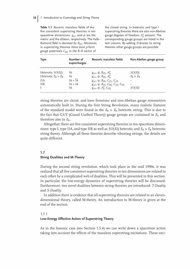
Table 1.1 Bosonic massless fields of thefive consistent superstring theories in tenspacetime dimensions. g μν and φ are themetric and the dilaton, respectively. The Kalb–Ramond field is denoted by B(2). Moreover,in superstring theories there exist p-formgauge potentials C(p) in the R–R sector of

the closed string. In heterotic and type Isuperstring theories there are also non-Abeliangauge degrees of freedom Aa

μ present. Thecorresponding gauge groups are listed in thelast column. By adding D-branes to stringtheories other gauge groups are possible.

Type Number of Bosonic massless fields Non-Abelian gauge groupsupercharges

Heterotic SO(32) 16 g μν, φ, B(2), Aaμ SO(32)

Heterotic E8 ~ E8 16 g μν, φ, B(2), Aaμ E8 ~ E8

IIA 16 + 16 g μν, φ, B(2), C(1) , C(3) –IIB 16 + 16 g μν, φ, B(2), C(0) , C(2), C(4) –I 16 g μν, φ, Aa

μ, C(2) SO(32)

string theories are chiral, and have fermions and non-Abelian gauge symmetriesautomatically built in. During the first String Revolution, many realistic featuresof the standard model were found in the E8 ~ E8 heterotic string. This is due tothe fact that GUT (Grand Unified Theory) gauge groups are contained in E6 andtherefore also in E8.

Altogether, there are five consistent superstring theories in ten spacetime dimen-sions: type I, type IIA, and type IIB as well as SO(32) heterotic and E8 ~ E8 heteroticstring theory. Although all these theories describe vibrating strings, the details arequite different.

1.7String Dualities and M-Theory

During the second string revolution, which took place in the mid 1990s, it wasrealized that all five consistent superstring theories in ten dimensions are related toeach other by a complicated web of dualities. This will be presented in this section.In particular, the low-energy dynamics of superstring theories will be discussed.Furthermore, two novel dualities between string theories are introduced: T-Dualityand S-Duality.

In addition there is evidence that all superstring theories are related to an eleven-dimensional theory, called M-theory. An introduction to M-theory is given at theend of the section.

1.7.1Low-Energy Effective Action of Superstring Theory

As in the bosonic case (see Section 1.5.4) we can write down a spacetime actiontaking into account the effects of the massless superstring excitations. These exci-

1.7 String Dualities and M-Theory 29

tations are listed in table 1.1. Since the effective supersymmetric action necessarilyincorporates gravity 9), the theory is called supergravity.

The low-energy effective action for type IIA and type IIB superstring theories arecalled type IIA and type IIB supergravity, respectively. As an example, we consid-er the action of type IIB supergravity. Type IIB superstring theory consists of thefollowing closed-string states at the massless level: the metric g μν, the NS–NS Kalb–Ramond field Bμν, the dilaton φ as well as the p-form R–R potentials C(0), C(2), andC(4). Moreover, we define as linear combinations of these fields the axion-dilatonscalar τ as well as the complex three-form G(3) by

τ = C(0) + i e–φ, G(3) = F(3) – τH(3) . (1.115)

Here, F(3) and H(3) are the field strength of C(2) and B(2), that is F(3) = dC(2) andH(3) = dB(2). The field strength of C(4) is given by F(5) = dC(4). More important isthe self-dual combination

F(5) == F(5) +12

B(2) ∧ F(3) –12

C(2) ∧ H(3) . (1.116)

The type IIB supergravity action in the Einstein frame then reads

SIIB =1

2κ210

Zd10x

√–g

"R –

|∂μτ|22(Imτ)2 –

|G(3)|212Imτ

–|F(5)|24 · 5!

)

+1

8iκ210

ZC(4) ∧ G(3) ∧ G(3)

Imτ, (1.117)

where the ten-dimensional gravitational coupling is 2κ210 = 16πG10 =1/(2π)(2πls)8g2

sand ls =

√α′ is the string length. Moreover, we have to impose the self-duality con-

straint of F(5) at the level of the equations of motion by hand, that is �F(5) = F(5),where � denotes the Hodge star operator.

1.7.2T-Duality

T-Duality (or target space duality) denotes the equivalence between two superstringtheories compactified on different background spacetimes. Let us consider bosonicstring theory compactified on a circle, that is the coordinate X 25 is periodicallyidentified in the following way,

X 25 ~ X 25 + 2πR . (1.118)

9) These effective spacetime theories are notonly invariant under global supersymmetrytransformations, but also under local ones.Since the commutator of two supersymmetry

transformations is a translation, the theory isalso invariant under local diffeomorphismsand therefore contains gravity.


1.7.2.1T-Duality of Closed StringsNow let us restrict ourselves to closed strings. The embedding function X 25(τ, σ)has to satisfy the periodicity condition

X 25(τ, σ + 2π) = X 25(τ, σ) + 2mπR , (1.119)

where R is the radius of the circle and m is an arbitrary integer. The number mcounts how often the closed string winds around the compactified direction X 25

and is therefore called the winding number. In the noncompactified directions, themode decomposition (1.71) and (1.72) for the right and left-moving modes can beused subject to p μ

R = p μL . In the compactified direction the same mode decomposi-

tion can be applied, however now with p25R =/ p25

L . Omitting the oscillatory terms, wehave the decomposition

X25R (τ – σ) =

12

x μ0 + α′p μ

R(τ – σ) + . . . ,

X25L (τ + σ) =

12

x μ0 + α′p μ

L (τ + σ) + . . . . (1.120)

Since X 25 = X 25L + X 25

R , the periodicity condition reads

α′(p25L – p25

R ) = mR . (1.121)

Since the X 25 direction is compactified, the center-of-mass momentum p25R + p25

L isquantized in units of 1/R, that is

p25L + p25

R =nR

. (1.122)

Thus, p25R and p25

L are given by

p25L =

12

„nR

+mRα′

«, (1.123)

p25R =

12

„nR

–mRα′

«. (1.124)

We are now interested in the spectrum of the closed-string states. First of all, thelevel-matching condition (see Section 1.5.2) for the closed string is modified,

N – N = nm , (1.125)

and the mass formula for string states reads

M2 =„

mRα′

«2

+“ n

R

”2+

2α′`N + N – 2

´. (1.126)

However, this is not the whole story. The closed-string sector has a remarkable sym-metry. Considering the mass formula, it turns out that the closed-string spectrumfor a compactification with radius R is identical to the closed-string spectrum for


a compactification with radius R = α′/R if we interchange the winding number mand momentum number n,

R ↔ R =α′

R, (1.127)

(n, m) ↔ (m, n) . (1.128)

Although here we have described the proof for T-duality only for free strings, it canbe shown that T-duality of closed strings is an exact symmetry at the quantum levelalso if interactions are included.

In fact it is not possible to distinguish between both compactifications. Note thatif R is large, then the dual radius R is small. This is a remarkable feature, which isnot present in usual field theories of point-like particles. Since T-duality exchangesthe winding number on the circle with the quantum number of the corresponding(discrete) momentum, it is clear that this symmetry has no counterpart in ordi-nary point particle field theory, as the ability of closed strings to wind around thecompact dimension is essential.

1.7.2.2T-Duality of Open StringsAt first sight, it seems that T-duality does not apply to theories with open strings,since open strings do not have a winding sector. However, this is only apparentlyso [22]. T-duality can be restored in the open-string sector with the help of D-braneswhich are hyperplanes where open strings end. By applying T-duality, not only theradius of the compactified dimension changes, but also the dimension of the D-brane.

To see this, let us consider the propagation of open bosonic strings in a spacetimewhich is compactified in the X 25 direction. Furthermore, we assume for simplicitythat we have a space-filling D25-brane, that is the endpoints of the string can movefreely. As it was in the case of closed strings, the center-of-mass momentum inthe compactified direction is quantized, that is p25 = n/R and contributes termsof the form n2/R2 to the mass formula of string states. However, this contributionchanges if we apply the T-duality rules of closed strings only. Since the dual radiusis R = α′/R, the contribution to the mass formula changes to n2R2/α′ 2.

T-duality can be restored in the open-string sector by considering D-branes. In-stead of the D25-brane described above, consider now a D24-brane in the dualtheory, which does not wrap the X 25-direction. Because of the Dirichlet boundaryconditions, we have no momentum states in the compact direction. In addition, theendpoints of the open string must remain attached to points with x25 = x25

0 + 2πnR,where x25

0 is the position of the D24-brane in the compactified direction. Therefore,we get winding states in the dual theory which contribute to the mass formula by

„nRα′

«2

=“ n

R

”2. (1.129)

This is precisely the contribution of the momentum states in the original theorywith a space-filling D25-brane.


Therefore, T-duality is an exact symmetry of the open-string sector, if the dimen-sion of the D-brane is also changed. This means that the type of boundary condi-tions of open strings (Neumann or Dirichlet) has to be exchanged in the directionin which T-duality is performed.

As an example consider a D24-brane stretched along the coordinates X 0, X 1, . . . ,X 24. In these directions Neumann boundary conditions for open strings are im-posed. Moreover, in the X 25-direction open strings will satisfy Dirichlet boundaryconditions. Assuming that the X 24 and X 25 directions are compactified on circleswith radius R24 and R25, respectively, we can apply T-duality to both compact di-rections. If we perform a T-duality along X 25, the open strings in the dual the-ory in the X 25-direction obey also Neumann boundary conditions. Therefore, inthe dual theory a D25-brane exists and the radii of the two compactified direc-tions are given by R24 and α′/R25, respectively. If we apply a T-duality along X 24

instead, the open strings no longer satisfy Neumann boundary conditions in theX 24-coordinate. Therefore, we are left with a D23-brane in the dual theory, which iscompactified on circles with radii α′/R24 and R25.

1.7.2.3T-Duality in Superstring TheoryUp to now we have only discussed the rules of T-duality in bosonic string theory.However, T-duality is also an exact symmetry of superstring theories. In fact T-Duality relates the following superstring theories:

– Heterotic SO(32) superstring theory on a circle with radius R and heteroticE8 ~ E8 superstring theory on a circle with radius α′/R.

– Type IIA superstring theory on a circle with radius R and type IIB superstringtheory on a circle with radius α′/R.

1.7.3S-Duality

S-duality is a strong–weak coupling duality, in the sense that a superstring theoryin the weak coupling regime is mapped to another strongly coupled superstringtheory. S-duality relates the string coupling constant gs to 1/gs in the same way thatT-duality maps the radii of the compactified dimension R to α′/R.

The most prominent example where S-duality is present is type IIB superstringtheory. This theory is mapped to itself under S-duality. This is due to the fact thatS-duality is a special case of the SL(2,�) symmetry of type IIB superstring theory:in the massless spectrum of type IIB superstring theory, the scalars φ and C(0)

and the two-form potentials B(2) and C(2) are present in pairs. Arranging the R–Rscalar C(0) and the dilaton φ in a complex scalar τ = C(0) + i exp(–φ), the SL(2,�)symmetry of the equations of motion of type IIB supergravity (see (1.117)) actsas

τ → aτ + bcτ + d

, (1.130)


with the real parameter a, b, c, d satisfying ad – bc = 1. Moreover, the R–R two-formpotential C(2) and the NS–NS B(2) transform according to

B(2)

C(2)

!→

d –c–b a

! B(2)

C(2)

!. (1.131)

Because of charge quantization, this symmetry group breaks down to SL(2,�) ofthe full superstring theory. A particular case of the above symmetry is S-duality. Ifthe R–R scalar C(0) vanishes, the coupling constant gs = exp(φ) of type IIB super-string theory can be mapped to 1/gs by the SL(2,�) transformation with a = d = 0,and b = –c = 1, that is

φ → –φ , B(2) → C(2) , C(2) → –B(2) . (1.132)

Note that the SL(2,�) duality of type IIB superstring theory is a strong–weak cou-pling duality relating different regimes of the same theory.

Since the NS–NS field B(2) couples to the fundamental string, the fundamentalstring carries one unit of B(2) charge, but is not charged under the NS–NS two-form field C(2). However, there are also solitonic strings which are charged underthe NS–NS two-form field C(2), but not under the Kalb–Ramond field B(2). Theseobjects are D1-branes (see also Section 1.8). Under S-duality, a fundamental stringis transformed into a D1-brane and vice versa. Moreover, a general SL(2,�) trans-formation maps the fundamental string into a bound state (p, q), carrying p unitsof NS–NS charge and q units of R–R charge.

1.7.4Web of Dualities and M-Theory

So far we have seen that type IIA and type IIB superstring theory are related byT-duality. The same applies to the two heterotic string theories. Moreover, we alsodiscussed S-duality in type IIB superstring theory. In contrast to T-duality, S-dualityis a strong–weak coupling duality gs → 1/gs, and therefore the role of fundamentalstrings and D1-branes are exchanged. In the strong coupling limit, D1-branes arenow the fundamental degrees of freedom since their tension τD1 = (2πα′gs)–1 issmaller than the tension τ = (2πα′)–1 of the fundamental string. Another examplefor S-duality are heterotic SO(32) and type I superstring theory. To be more precise:the strong coupling limit of type I superstring theory is weakly coupled SO(32)heterotic string theory.

S-duality and T-duality are embedded into a larger symmetry group, U-duality [23].By using this U-duality, it was realized in 1995 that the strong coupling regime ofall five consistent string theories in ten spacetime dimensions is mapped to someweakly coupled limit of another theory ([24], for a review see [25]). For this pic-ture to be self-contained, one has to include also eleven-dimensional supergravity.It is believed that all five consistent string theories can be unified into an eleven-dimensional parent theory, called M-theory. Although up to now a precise definition


of M-theory is not available, we know that the low-energy effective action of thistheory is given by the unique eleven-dimensional supergravity.

At strong coupling fundamental strings are no longer the fundamental degreesof freedom of superstring theory. Therefore, we can not expect that only ten-dimensional target spacetimes are consistent since this was derived by consideringthe trace of the energy–momentum tensor of the world-sheet of fundamentalstrings.

1.7.4.1Type IIA String Theory and M-TheoryLet us explore the connection between type IIA superstring theory and M-theoryin more detail. The first evidence of such a connection was found by [26]: typeIIA supergravity, which is the low-energy limit of type IIA superstring theory, canbe derived from a Kaluza–Klein reduction of eleven-dimensional supergravity. Thebosonic spectrum of eleven-dimensional supergravity consists of a metric GMN anda three-form potential A(3) with components AMNP. A Kaluza–Klein reduction toD = 10 is performed by putting the eleventh coordinate X10 on a circle of radiusR10. Decomposing the fields with respect to the ten-dimensional Lorentz group, wecan identify the field content of type IIA supergravity. The metric GMN and three-form potential A(3) of eleven-dimensional supergravity is related to the dilaton φ,to the metric g μν, and to the R–R-potentials C(1) and C(3) in the following schematicway, symbolized by ~:

GMN → φ ~ G10 10 ,

Cμ ~ Gμ 10 ,

g μν ~ Gμν ,

AMNP → Bμν ~ Aμν10 ,

Cμνρ ~ Aμνρ , (1.133)

where μ, ν, ρ = 0, . . . , 9. Moreover, the ten-dimensional fields are independentof the eleventh, internal coordinate X10. To be precise, the metric of the eleven-dimensional spacetime is determined by the field content of type IIA superstringtheory

ds2 = GMN dxM dxN = exp(–2/3φ)g μν dx μ dxν + exp(4/3φ)`

dx11 + Cμ dx μ´2.

(1.134)

Therefore, we see that a distance measured in ten-dimensional spacetime is multi-plied by g–1/3

s in eleven-dimensional spacetime. The Planck length lp is determinedby the string length ls =

√α′,

lp = g1/3s ls . (1.135)

Integrating out the eleventh dimension yields a prefactor in front of the action,relating the ten- and eleven-dimensional gravitational coupling constants κ10 and


κ11 by

κ210 =

κ211

2πR10. (1.136)

Using the eleven-dimensional gravitational constant

16πG11 = 2κ211 =

12π

(2πlp)9 , (1.137)

we can deduce the radius R10 of the compactified direction,

R10 = g2/3s lp = gsls = gs

√α′ . (1.138)

For small string coupling constant gs the radius R10 of the compactified direction inunits of the string length is small and the spacetime is effectively ten-dimensional.However, for large string coupling constants the spacetime is eleven-dimensional.

As discussed in the last paragraph, the low-energy limit of type IIA superstringtheory, which is given by type IIA supergravity, can be obtained by a Kaluza–Kleinreduction of eleven-dimensional supergravity on a circle S1. However, the relationbetween type IIA supergravity and M-theory is much deeper. Let us match nonper-turbative objects on both sides. In the nonperturbative part of its spectrum eleven-dimensional supergravity has M2- and M5-branes, which are charged under thefour-form field strength G(4) = dA(3). The nonperturbative spectrum of type IIAsupergravity contains stable Dp-branes with p even as well as NS5-branes.

Let us consider some examples to see how D-branes and M-branes are related.The D0-branes of type IIA are mapped to Kaluza–Klein of the massless supergrav-ity multiplet. An evidence for this statement is the mass of the two states. SinceD0-branes are nonperturbative, their mass is proportional to g–1

s . A bound state ofn D0-branes therefore has mass ~ n/gs. This matches precisely with mass statesof Kaluza–Klein excitations on a circle with radius gs in units of the string length.Moreover, the fundamental string and D2-branes can be related to M2-branes bydimensional reduction of x10: in the case of the fundamental string the M2 braneis wrapped on the compactified coordinate x10. Performing a dimensional reduc-tion we obtain a fundamental string. If the M2 brane is not wrapped along thecompactified dimension we get a D2-brane. In addition, D4 and NS5 branes can bemapped to M5-branes of M-theory. For further details see [26].

In summary, we gave evidence that type IIA superstring theory is dual to M-theory on S1, where the radius of the circle in units of the string length is givenby the string coupling constant gs. This implies that the perturbative regime ofstring theory is ten-dimensional because the radius of the compactified coordinateis small. Moreover, in the nonperturbative regime, the radius becomes large andthe coordinate is effectively decompactified.

1.7.4.2Heterotic E8 ~ E8 String Theory and M-TheoryA similar picture arises in the strong coupling limit of the heterotic E8 ~ E8 stringtheory, which is equivalent to M-theory on the orbifold S1/�2 [27], that is we con-sider only string states which are even under the �2-symmetry x10 → –x10 and


A(3) → –A(3) of M-theory on �9,1 ~ S1. The orbifold S1/�2, can be viewed as a linesegment from x10 = 0 to x10 = πR10, where R10 is related to the string coupling con-stant as in type IIA superstring theory. The super Yang–Mills fields are located atthe fixed points of the orbifold, x10 = 0 and x10 = πR10. Therefore, these boundariesof the eleven-dimensional spacetime are called “end-of-the-world-9-branes”. Eachof the branes carry non-Abelian gauge fields with gauge group E8. In this picturethe product gauge group E8 ~ E8 can be understood. Moreover, the fundamentalstrings of heterotic E8 ~ E8 string theory are precisely the cylindrical M2-branessuspended between the “end-of-the-world-9-branes”.

This picture of strongly coupled heterotic E8 ~ E8 string theory is the startingpoint of heterotic M-theory. By compactifying (usually on Calabi–Yau manifolds) tofour spacetime dimensions it is possible to investigate phenomenologically inter-esting strong coupling effects. For more details see Chapter 8.

1.8D-Branes

So far we have considered D-branes as hyperplanes where fundamental strings canend. This is a microscopic point-of-view, since D-branes are defined as boundariesof world-sheets of open strings. The massless string excitations of open stringsending on D-branes can be described in general by a supersymmetric (non-)Abeliangauge theory. The precise form of the effective action is discussed in Section 1.8.1.

In addition, D-branes are also solitonic solutions to the macroscopic equationsof motion for the low-energy theory of superstring theory, governed effectivelyby supergravity. In that macroscopic point-of-view D-branes are objects such asblack holes, cosmic strings, monopoles, which curve the surrounding spacetime.These D-branes are a further ingredient to superstring theory besides fundamentalstrings. Moreover, BPS D-branes carry charges of the R–R p-form gauge fields C(p).Because of charge conservation BPS D-branes are stable. In type IIA/IIB super-string theory Dp-branes with p even/odd are BPS since in this superstring theoryRR gauge potentials C(p+1) are present to which Dp-branes couple [28]. However,unlike fundamental strings, D-branes are nonperturbative since the tension andtherefore also the energy scales as 1/gs. This aspect of D-branes is investigated inSection 1.8.2.

1.8.1Effective Action of D-Branes

The dynamics of the massless open-string modes ending on one Dp-brane (or onone anti-Dp-brane) is described by an effective action

SDp = SDBI ± SCS , (1.139)

consisting of a Dirac–Born–Infeld (DBI) and a Chern–Simons (CS) action. Therelative sign between the DBI and CS part of the action depends on whether it is

1.8 \textitD-Branes 37

a Dp or anti-Dp-brane (also denoted by Dp-brane). The plus sign corresponds toa Dp-brane.

The interaction of the NS–NS massless fields g μν, Bμν, and φ as well as the NSfield strength Fab on the Dp-brane are given by the DBI action

SDBI = –μp

ZDp

dp+1� e–P[φ]q

– det`P[g]ab + Fab

´, (1.140)

where Fab = 2πα′Fab +P[B]ab and P[B]ab,P[g]ab are the pullback of Bμν and g μν, thatis

P[B]ab = ∂a X μ∂bX νBμν , P[g]ab = ∂a X μ∂bX νg μν , (1.141)

with ∂a = ∂/∂�a and a, b, = 0, . . . , p. The constant μp is given by μp = (2π)–pα′ –(p+1)/2

for type II theories.Expanding the DBI action by using det(�+ M) = 1 – 1/4 tr(M2) for antisymmetric

matrices M we see that the DBI action is a generalization of a Yang–Mills action

SDBI � (2πα′)2

4

ZDp

dp+1�FabFab . (1.142)

Moreover, we consider only a constant dilaton field φ. The D-brane tension is de-fined by τp = μp/gs.

The Chern–Simons part of the action describes the interaction of the R–R fieldsas well as the interaction with the NS–NS fields

SCS = μp

ZDp

Xq

P ˆC(q+1)˜ ∧ tr eF . (1.143)

The integral is restricted only to p + 1-forms.The DBI and CS part together form the relevant action for a single Dp-brane at

leading classical order in the string coupling gs, that is at disk level, and at leadingorder in the derivatives.

Furthermore, the DBI and CS action can be generalized to coincident Dp-branes,giving rise to the non-Abelian DBI and CS actions. Further details can be foundin [29] or in the book [7]. Moreover, coincident Dp-branes ending on Dq-branes(q > p) can be described by excitations of massless fields on the higher-dimensionalD-brane as well as by a dielectric effect on the lower-dimensional D-branes. Fordetails involving coincident D1-branes ending on a D3-brane see [30].

Besides BPS D-brane configurations there also exists non-BPS D-branes (fora review see [31]). A prominent example for non-BPS D-brane configurations areDp – Dp systems, which are also important in brane-inflation models (see Chap-ter 2 for more details). Since Dp- and Dp-branes are oppositely charged, the branesattract each other. If the spatial distance between the Dp- and the anti-Dp-brane isof the order of the string length, a tachyon [32] will be present in the spectrum ofopen strings. This tachyon indicates an instability of the Dp – Dp-brane system;indeed the Dp- and anti Dp-brane will annihilate to closed-string radiation.

The effective action of non-BPS D-brane configurations involves not only themassless string excitations but also the tachyon – a complex scalar field (for a pro-posal of an effective action for the Dp – Dp see [33]).


1.8.2D-Branes as Charged BPS Objects

In superstring theories Dp-branes carry conserved charges of topological nature.In particular D-branes are described at low energies by solitonic supersymmetricsolutions of the effective supergravity equations of motion that carry R–R charge,which is given by (1.149). Splitting the ten-dimensional spacetime into the world-volume directions a, b = 0, . . . , p and the transverse directions i, j = p + 1, . . . , 9 thesolution for the metric, dilaton, and the R–R p-form potentials are given by

ds2 = H–1/2p ηab dxa dxb + H1/2

p dxi dxi , (1.144)

eφ = gs H(3–p)/4p , (1.145)

C(p+1) =“

H–1p – 1

”g–1

s dx0 ∧ dx1 ∧ · · · ∧ dxp , (1.146)

Bμν = 0 , (1.147)

where the harmonic function Hp(r) with r 2 = δijxix j is

Hp = 1 +“ rp

r

”7–p. (1.148)

Whereas C(q+1) vanishes for a Dp-brane (q =/ p), the Dp-brane induces a nontrivialp + 2-form field strength F(p+2) = dC(p+1) as well as a nontrivial dilaton for p =/ 3.The charge of a Dp-brane can be calculated by integrating the R–R flux through the(8 – p)-dimensional sphere at infinity in the transversal dimensions,

Q =Z

S8–p�F(p+2) , (1.149)

where � is the Hodge operator.

1.9Compactification

We have seen that superstring theory is consistent in ten dimensions. Therefore,it remains necessary to find a way to obtain four-dimensional physics, and in par-ticular the Standard Model of elementary particle physics, from superstring theory.For this purpose, two different approaches are pursued:

– Kaluza–Klein compactificationsIn the Kaluza–Klein compactifications it is assumed that the ten-dimensio-nal target spacetime of superstring theories has four uncompactified largedimensions, which correspond to the real world. The remaining six dimen-sions are compactified on a length scale lc. For observations at energies E <<1/lc the six compactified directions are invisible, though the topology and thelength scales of the compactification have influence on the spectrum of the

1.9 Compactification 39

four-dimensional theory at low energies. We assume that the spacetime canbe written as a product

M10 = �3,1 ~ M6 , (1.150)

where �3,1 is the four-dimensional Minkowski spacetime. Promising candi-dates for M6 are Calabi–Yau manifolds. Because of the special properties ofthese manifolds, the effective four-dimensional theory at low energies pre-serves some supersymmetry.

– Brane-world scenariosIn this approach the Minkowski spacetime of the four uncompactified di-mensions is identified with a defect embedded into ten-dimensional space-time. The defect is generated by intersecting and coincident D-branes. Inbrane-world models so-called warped compactifications are studied, where thelength scale of the four-dimensional Minkowski spacetime depends on thecoordinates of the compactified dimension. However, Poincaré invariance ofthe four-dimensional Minkowski spacetime is preserved. The typical metricof a warped compactification is given by

ds2 = e2A(y)g μν dx μ dxν + e–2A(y)gab dy a dy b , (1.151)

where g μν is the metric of the four-dimensional spacetime. We see that incontrast to (1.150), the four and six-dimensional spaces are no longer topo-logically independent.

1.9.1String Theory on Calabi–Yau Manifolds

Before we discuss features of string theory on Calabi–Yau manifolds, we have todefine Kähler and Calabi–Yau manifolds. Kähler manifolds are complex manifoldsfor which the exterior derivative of the fundamental form, associated with the givenHermitean metric vanishes. The metric on the Kähler manifold locally satisfies

Gij =∂2K

∂zi∂zj, (1.152)

where K is the so-called Kähler function.Calabi–Yau n-folds are Kähler manifolds in n complex dimensions with the ad-

ditional topological property of vanishing first Chern class, c1 = 0. Any compactKähler manifold with c1 = 0 admits a Kähler metric with SU(n) holonomy and isnecessarily Ricci flat. See [34] for the precise definition. Examples of Calabi–Yaumanifolds are

– The complex plane � and the two-torus T2 in two (real) dimensions. Theseare all examples in two dimensions since any compact Riemannian surface,except the torus T2, is not a Calabi–Yau manifold.

– In four (real) dimensions there are two compact Calabi–Yau manifolds: thefour-torus T4 and K3. Examples of noncompact Calabi–Yau manifolds are�

2 ~ T2 and �4.


– In six (real) dimensions there are many Calabi–Yau three-folds known. Infact, the number of Calabi–Yau three-folds may even be infinite since thereis no mathematical proof for the finiteness of the number up to now.

1.9.1.1Low-Energy Effective TheoryLet us discuss the properties of four-dimensional gauge theories which are ob-tained from compactifications. Compactifying ten-dimensional superstring theoryon Calabi–Yau three-folds breaks 3/4 of supersymmetry. Therefore the effectivefour-dimensional theory has N = 1 supersymmetry for heterotic string theoriesand N = 2 for type II superstring theories. The low-energy effective theory in fourspacetime dimensions for type II superstring theories consists of

– N = 2 supergravity multiplet,– N = 2 Abelian vector multiplets,– N = 2 hypermultiplets.

The number of vector and hypermultiplets depend on topological properties of theCalabi–Yau manifolds, in particular on the Hodge numbers hp,q.

By adding D-branes to the compactification setup we may obtain non-Abeliangauge theories in four dimensions. Compactifications of type II superstring theo-ries are often inconsistent or unstable due to uncanceled charges of D-branes ordue to fluxes. A remedy is to perform a orientifold projection10). In particular thecharges and tensions of D-branes are canceled by orientifold-planes (so-called O-planes). Orientifold projections ensure that the four-dimensional low-energy effec-tive action preserves N = 1 supersymmetry. The bosonic part of N = 1 supergravitycoupled to chiral and vector multiplets is given by

L =1

2κ4R – Gij(φ, φ)DμφiD μφ j – V

–18

Re fab(φ)F aμνF bμν –

18

Im fab(φ)εμνρσF aμνF b

ρσ . (1.153)

φi are the scalar fields of the chiral multiplet and Fμν is the field strength tensor ofthe gauge fields of the vector multiplet. Moreover, Dμ is the covariant derivative andGij is the metric of the scalar target space11), which is given by the Kähler potentialK(φ, φ),

Gij =∂2K(φ, φ)∂φi∂φ j

. (1.154)

The gauge-kinetic function fab(φ) in (1.153) is an arbitrary analytic function of thescalar fields φi. If some scalar fields φi acquire vacuum expectation values dynam-ically, this may generate vacuum expectation values for fab(φ). This controls the

10) For more details see [35].11) The inverse matrix of Gij is as usual denoted

by upper indices.

1.9 Compactification 41

coupling constant gab of the gauge fields12), since

Re fab = g–2ab . (1.155)

The last ingredient of the general form of N = 1 supergravity in four spacetimedimensions is the scalar potential V , which consists of two parts referred to as D-and F-term potentials:

V = VF + VD . (1.156)

The F-term potential is determined by the holomorphic superpotential W(φ),

VF = eK/M2pl

“GijDiWDjW – 3M2

pl|W|2”

, (1.157)

where the covariant derivative of the superpotential is defined by

DiW = ∂iW + M2plGiW with Gi =

∂K(φ, φ)∂φi . (1.158)

The D-term potential VD is expressed in terms of the auxiliary Da-fields of the vectormultiplet,

VD =12`Re(f )–1´

ab Da Db . (1.159)

In contrast to global supersymmetric field theories, the scalar potential V doesnot have to be zero in a supersymmetry preserving vacuum since a supersymmetricvacuum has to satisfy Da = DiW = 0. Therefore, the scalar potential (1.157), (1.158)in a supersymmetric vacuum has the value

V = –3M2pl|W|2 exp

“K/M2

pl

”. (1.160)

Since the scalar potential is negative and the scalar potential is related to the cos-mological constant, the vacuum has negative cosmological constant. This is goodnews, since states with broken supersymmetry (i.e. Da =/ 0 or DiW =/ 0) can havean almost zero scalar potential and therefore a tiny positive cosmological constant.

1.9.2String Theory on Orbifolds

Even for simple examples of Calabi–Yau manifolds (for example K3), the metric isnot known explicitly. Therefore, one generally considers string theory on orbifoldssince there effects of singular limits of Calabi–Yau manifolds can be studied. More-over, the metric of orbifolds is explicitly known. For more details see the review [35].

The definition of an orbifold is as follows. Let X be a smooth manifold witha discrete isometry group G. An orbifold is the quotient space X/G. The points ofX/G are precisely the points of X, whereas two points x1 and x2 are identified ifthey are connected by a group transformation. Simple examples are

12) In renormalizable field theories we have onlyone gauge coupling for the gauge fields sincegab , i.e. gab = g δab.


– S1/�2, that is opposite points on a circle will be identified. This gives aninterval.

– The orbifold�/�N is a cone, since points of the complex plane which can bemapped onto each other by a rotation by (2πk)/N are identified.

We see that orbifolds can be singular. This generally happens if nontrivial group el-ements leave points of X invariant. Although general relativity is ill-defined on sin-gular spaces, it is possible to define string theory consistently on orbifolds. Thereare two types of strings on orbifolds:

– untwisted states, that is states which exist on X and are invariant under thegroup G.

– twisted states are new closed-string states, which satisfy the condition X μ(τ, σ+2π) = gX μ(τ, σ), where g ∈ G. The twisted sectors are labeled by the particulargroup element g. Untwisted strings correspond to g = 1. A generic feature oforbifolds is the localization of strings of the twisted sector at the orbifoldsingularities.

Only by including twisted states into the string spectrum can strings propagateconsistently on spaces with orbifold singularities. Furthermore, string theories onorbifolds X/G have more broken supersymmetry than on X, which again makesthem interesting for the phenomenology of string theory.

1.9.3String Moduli and Their Stabilization

Some of the Calabi–Yau manifolds are smoothly related by deformations of para-meters characterizing the shape and size. These parameters are called string mod-uli. Examples are expectation values of the dilaton field, the values of couplingconstants, expectation values of Wilson lines around nontrivial cycles and variousparameters (e.g. the radii and the complex structure) describing the shape of thecompactification manifold.

As a simple example let us discuss the moduli space of bosonic string theorycompactified on a circle S1 along the X 25-direction. In that case the relevant pa-rameter describing the compactification is the radius R of the compactified direc-tion. Whereas in field theory every radius leads to different physics, the situationin string theory is different due to T-duality (see Section 1.7.2). Backgrounds withlarge radius (in string units) are transformed into backgrounds with small radiusR (in string units). Therefore, there exists a smallest (respectively biggest) radiusR0 =

√α′ and the moduli space is M = {R u R0} or equivalently M = {R v R0}.

In a more formal way the moduli space can be written in the form

M = {R ∈ �+/�2} . (1.161)

In string theory the parameters of the moduli space describe different vacuumconfigurations and can be related to vacuum expectation values of massless scalarfields. In the case of a circle compactification the vacuum expectation value of the

1.10 String Thermodynamics 43

scalar

|Φ〉 = α25–1α25

–1|0〉 (1.162)

is related to the radius of the circle.This is a general rule of perturbative string theory: moduli can be considered

as massless scalar fields on the string world-sheet. However, it is not possible topredict the vacuum expectation value of the moduli, since the potential is flat inthe four-dimensional effective theory. This is the moduli stabilization problem. Onepossibility to solve it is to use warped background compactifications. Nontrivialwarp factors in the metric are obtained by nonvanishing fluxes, by branes, and byhigher-order corrections to low-energy supergravity actions. For details see Chap-ters 2 and 3 in this book or the review [35].

1.10String Thermodynamics

In this section, we introduce thermodynamics of open bosonic strings ending ona Dp-brane. For simplicity we consider only bosonic open strings that do not carryspatial momentum. To compute the entropy in the microcanonical ensemble, wehave to count the string states with given energy E. This is done by determiningall partitions of the string level number N associated with the string energy E =√

N – 1/√

α′. The result for the number of string states is (see also [2])

Ω(E ) � E –γ exp(4π√

α′E ) , (1.163)

with γ = (25 – p)/2. Calculating the entropy by using S(E ) = kB ln Ω(E ), we obtaina relation between the entropy S and the energy E which is asymptotically linearfor high energies E >> 1,

S(E ) = –γkB ln E + 4π√

α′kBE . (1.164)

This is an unusual behavior in statistical mechanics since it immediately leads toa constant temperature at high energies,

1�

= k–1B

∂S∂E

= –γE

+ 4π√

α′ , (1.165)

which is called the Hagedorn temperature TH and is given by TH = (4π√

α′kB)–1.Inverting the equation (1.165) we obtain

E(T ) = γ„

1kBTH

–1

kBT

«–1

. (1.166)

For T → TH the energy E diverges. For closed strings and open superstrings thesame relation up to numerical factors hold.


In the canonical ensemble the string partition function Zstring also diverges ifthe temperature T approaches the Hagedorn temperature. The partition functionis well approximated by

Zstring � CTH – T

(1.167)

for T → TH. For more details and computations see for example [2].

1.11Gauge–Gravity Duality

Gauge–gravity dualities are dualities between a (quantum) theory of gravity on onehand, and a gauge theory in a spacetime with a lower number of dimensions onthe other. Gauge–gravity dualities may be viewed as a realization of the holographicprinciple, since the same amount of degrees of freedom is encoded in the higher-dimensional space as well as in the lower-dimensional. There is a one-to-one cor-respondence between gauge invariant operators in the gauge theory and fields inthe dual gravity theory. Moreover, gauge–gravity dualities are strong–weak couplingdualities in the sense that one theory is strongly coupled, whereas the other theoryis weakly coupled and therefore accessible to perturbation theory. For instance, byapplying gauge–gravity dualities, strongly coupled gauge theories can be investi-gated by mapping them to weakly coupled gravity theories. The most prominentexample of gauge–gravity duality is the duality between type IIB supergravity ona five-dimensional Anti-de Sitter (AdS) spacetime and N = 4 SU(N) super Yang–Mills theory on the conformal boundary of the Anti-de Sitter spacetime. This is thewell-known AdS/CFT correspondence conjectured by Maldacena in 1997 [36], inwhich the conformal field theory is N = 4 SU(N) super Yang–Mills.

The duality is motivated by looking at the two different aspects of D-branes as de-scribed in Section 1.8. On one hand D-branes can be viewed as hyperplanes whereopen strings end. The low-energy effective dynamics of open strings is describedby a gauge theory. On the other hand D-branes are charged BPS solutions of su-pergravity curving the surrounding spacetime. For the duality involving N = 4Yang–Mills theory described above, the map between gauge and gravity theory isobtained by considering the two aspects for the case of D3-branes: in a particularlow-energy decoupling limit [36], open strings ending on D3-branes give rise toN = 4 super Yang–Mills theory on four-dimensional Minkowski spacetime. In thesupergravity picture, the low-energy limit gives rise to closed-string excitations inthe space AdS5 ~ S5. The degrees of freedom in both pictures are then identified.

This leads to the conjecture that gravitational theories and gauge theories de-scribe the same physics from different points-of-view. The interested reader is re-ferred to the reviews [37, 38] for further details. In Chapter 7, gauge–gravity duali-ties are applied to string cosmology.

1.12 Summary 45

1.12Summary

We have presented essential features of both cosmology and string theory whichwill be used in the subsequent chapters where string cosmology is introduced. Withthe material presented in this chapter, the reader is now equipped for studying thestring cosmology research topics in the subsequent chapters.

References

1 V. Mukhanov, Physical Foundations ofCosmology. Cambridge University Press,2005.

2 B. Zwiebach, A first course in string the-ory, Cambridge University Press (2004),558 p.

3 E. Kiritsis, String theory in a nutshell,Princeton University Press (2007), 588 p.

4 K. Becker, M. Becker, and J.H. Schwarz,String theory and M-theory: A modern in-troduction, Cambridge University Press(2007), 739 p.

5 M.B. Green, J.H. Schwarz, and E. Wit-ten, Superstring theory, Vol. I and Vol. II.Cambridge University Press, 1987.

6 J. Polchinski, String theory, Vol. I andVol. II. Cambridge University Press(1998), 402 p.

7 C.V. Johnson, D-branes. Cambridge Uni-versity Press, 2003.

8 L. McAllister and E. Silverstein, StringCosmology: A Review, Gen. Rel. Grav. 40(2008) 565 [arXiv:0710.2951 [hep-th]].

9 C.P. Burgess, Lectures on Cosmic Infla-tion and its Potential Stringy Realizations,PoS P2GC (2006) 008 [Class. Quant.Grav. 24 (2007) S795] [arXiv:0708.2865[hep-th]].

10 J.M. Cline, String cosmology, Lecturesgiven at Advanced Summer Instituteon New Trends in Particle Physics andCosmology, Sheffield, England, 19–23June 2006 and at Les Houches SummerSchool – Session 86: Particle Physics andCosmology: The Fabric of Spacetime, LesHouches, France, 31 Jul–25 Aug 2006.arXiv:hep-th/0612129 (www.arXiv.org).

11 M. Trodden and S.M. Carroll, TASIlectures: Introduction to cosmology,arXiv:astro-ph/0401547 (www.arXiv.org).

12 M. Gasperini: Elements of String Cos-mology. Cambridge University Press,2007.

13 A.A. Penzias and R.W. Wilson, Astro-phys. J. 142 (1965) 419.

14 E. Komatsu et al. [WMAP Collabora-tion], “Five-Year Wilkinson MicrowaveAnisotropy Probe (WMAP) Observa-tions: Cosmological Interpretation”, arX-iv:0803.0547 [astro-ph] (www.arXiv.org);K. A. Olive, TASI lectures: Dark matter,arXiv:astro-ph/0301505 (www.arXiv.org).

15 A.H. Guth, Phys. Rev. D 23, 347 (1981);A.D. Linde, Phys. Lett. B 108, 389(1982); A. Albrecht and P.J. Steinhardt,Phys. Rev. Lett. 48, 1220 (1982).

16 P.J.E. Peebles: The Large-Scale Structureof the Universe, Princeton UniversityPress, 1980.

17 A. Sen and B. Zwiebach, Tachyon con-densation in string field theory, JHEP 0003(2000) 002.

18 E. D’Hoker and D.H. Phong, The Geom-etry of String Perturbation Theory, Rev.Mod. Phys. 60 (1988) 917.

19 R.G. Leigh, Dirac–Born-Infeld Actionfrom Dirichlet Sigma Model, Mod. Phys.Lett. A 4 (1989) 2767.

20 N. Berkovits, ICTP lectures on covariantquantization of the superstring, arXiv:hep-th/0209059.

21 F. Gliozzi, J. Scherk, and D.I. Olive,Supersymmetry, Supergravity Theories AndThe Dual Spinor Model, Nucl. Phys. B122 (1977) 253.

46 References

22 J. Dai, R.G. Leigh and J. Polchinski,New Connections Between String Theories,Mod. Phys. Lett. A 4 (1989) 2073.

23 C.M. Hull and P.K. Townsend, Unity ofsuperstring dualities, Nucl. Phys. B 438,109 (1995).

24 E. Witten, String theory dynamics in vari-ous dimensions, Nucl. Phys. B 443 (1995)85 [arXiv:hep-th/9503124].

25 N.A. Obers and B. Pioline, U-duality andM-theory, Phys. Rept. 318, 113 (1999)

26 P.K. Townsend, The eleven-dimensionalsupermembrane revisited, Phys. Lett. B350 (1995) 184 [arXiv:hep-th/9501068].

27 P. Horava and E. Witten, Heterotic andtype I string dynamics from eleven di-mensions, Nucl. Phys. B 460 (1996) 506[arXiv:hep-th/9510209].

28 J. Polchinski, Dirichlet-Branes andRamond-Ramond Charges, Phys. Rev.Lett. 75 (1995) 4724 [arXiv:hep-th/9510017].

29 R.C. Myers, Dielectric-branes, JHEP 9912(1999) 022 [arXiv:hep-th/9910053].

30 N.R. Constable, R.C. Myers andO. Tafjord, The noncommutative bioncore, Phys. Rev. D 61 (2000) 106009[arXiv:hep-th/9911136].

31 J.H. Schwarz, TASI lectures on non-BPSD-brane systems, arXiv:hep-th/9908144.

32 T. Banks and L. Susskind, Brane —Antibrane Forces, arXiv:hep-th/9511194.

33 P. Kraus and F. Larsen, Boundary stringfield theory of the DD-bar system, Phys.Rev. D 63 (2001) 106004 [arXiv:hep-th/0012198].

34 B.R. Greene, String theory on Calabi-Yaumanifolds, arXiv:hep-th/9702155.

35 R. Blumenhagen, B. Körs, D. Lüst andS. Stieberger, Four-dimensional StringCompactifications with D-Branes, Ori-entifolds and Fluxes, Phys. Rept. 445, 1(2007)

36 J.M. Maldacena, The large N limit ofsuperconformal field theories and super-gravity, Adv. Theor. Math. Phys. 2 (1998)231

37 O. Aharony, S.S. Gubser, J.M. Malda-cena, H. Ooguri and Y. Oz, Large Nfield theories, string theory and gravity,Phys. Rept. 323 (2000) 183 [arXiv:hep-th/9905111].

38 E. D’Hoker and D.Z. Freedman, Super-symmetric gauge theories and the AdS/CFTcorrespondence, arXiv:hep-th/0201253.

1 Introduction to Cosmology and String Theory - … · 4 1 Introduction to Cosmology and String...

Documents

Transcript of 1 Introduction to Cosmology and String Theory - … · 4 1 Introduction to Cosmology and String...