1 Introduction - Assets - Cambridge University...
10
1 Introduction ‘Remote sensing’ is, broadly but logically speaking, the collection of information about an object without making physical contact with it. (The term was coined by Evelyn Pruitt of the US Office of Naval Research in the 1950s.) This is a simple definition, but too vague to be really useful (Campbell 2008), so for the purpose of this book we restrict it by confining our attention to the Earth’s surface and atmosphere, viewed from above using electromagnetic radiation. This narrower definition excludes such techniques as seismic, geomagnetic and sonar investigations, as well as (for example) medical and planetary imaging, all of which could otherwise reasonably be described as remote sensing, but it does include a broad and reasonably coherent set of techniques, nowadays often described by the alternative name of Earth observation. These techniques, which now have a huge range of applications in the ‘civilian’ sphere as well as their obvious military uses, make use of information impressed in some way on electromagnetic radiation ranging from ultraviolet to radio frequencies. One important casualty of our restricted definition of remote sensing is the use of spaceborne methods of measuring the Earth’s gravitational field. Although observa- tions from artificial Earth satellites have been used since the 1970s to measure the Earth’s gravity, our current (at the time of writing, in 2012) ability in this regard is a remarkable indication of the level of space technology. This is the GRACE (Gravity Recovery and Climate Experiment) mission, launched in 2002. Two satellites, each with a mass of around half a tonne, follow the same orbit 500 km above the Earth’s surface. They are approximately 220 km apart, and the distance between them is constantly monitored with an accuracy of 10 mm. This distance changes as the satellites cross regions of different gravitational field strength. The GRACE system is sensitive enough to respond to changes in groundwater in a large river basin. Data from the GRACE mission are described in Chapter 8. 1.1 A short history of remote sensing ................................................................................................................ The origins of remote sensing can plausibly be traced back to the fourth century BC and Aristotle’s camera obscura (or, at least, the instrument described by Aristotle in his Problems but perhaps known even earlier). Although significant developments in the Cambridge University Press 978-1-107-00473-3 - Physical Principles of Remote Sensing: Third Edition W. G. Rees Excerpt More information www.cambridge.org © in this web service Cambridge University Press
Transcript of 1 Introduction - Assets - Cambridge University...
1 Introduction
‘Remote sensing’ is, broadly but logically speaking, the collection of information about
an object without making physical contact with it. (The term was coined by Evelyn
Pruitt of the US Office of Naval Research in the 1950s.) This is a simple definition, but
too vague to be really useful (Campbell 2008), so for the purpose of this book we
restrict it by confining our attention to the Earth’s surface and atmosphere, viewed
from above using electromagnetic radiation. This narrower definition excludes such
techniques as seismic, geomagnetic and sonar investigations, as well as (for example)
medical and planetary imaging, all of which could otherwise reasonably be described
as remote sensing, but it does include a broad and reasonably coherent set of
techniques, nowadays often described by the alternative name of Earth observation.
These techniques, which now have a huge range of applications in the ‘civilian’ sphere
as well as their obvious military uses, make use of information impressed in some way
on electromagnetic radiation ranging from ultraviolet to radio frequencies.
One important casualty of our restricted definition of remote sensing is the use of
spaceborne methods of measuring the Earth’s gravitational field. Although observa-
tions from artificial Earth satellites have been used since the 1970s to measure the
Earth’s gravity, our current (at the time of writing, in 2012) ability in this regard is a
remarkable indication of the level of space technology. This is the GRACE (Gravity
Recovery and Climate Experiment) mission, launched in 2002. Two satellites, each with
a mass of around half a tonne, follow the same orbit 500 km above the Earth’s surface.
They are approximately 220 km apart, and the distance between them is constantly
monitored with an accuracy of 10 mm. This distance changes as the satellites cross
regions of different gravitational field strength. The GRACE system is sensitive enough
to respond to changes in groundwater in a large river basin. Data from the GRACE
mission are described in Chapter 8.
1.1 A short history of remote sensing................................................................................................................The origins of remote sensing can plausibly be traced back to the fourth century BC and
Aristotle’s camera obscura (or, at least, the instrument described by Aristotle in his
Problems but perhaps known even earlier). Although significant developments in the
Cambridge University Press978-1-107-00473-3 - Physical Principles of Remote Sensing: Third EditionW. G. ReesExcerptMore information
www.cambridge.org© in this web service Cambridge University Press
theory of optics began to be made in the seventeenth century, and glass lenses were
known much earlier than this, the first real advance towards our modern conception of
remote sensing came in the first half of the nineteenth century with the invention of
photography. For the first time, it became possible to record an image permanently and
objectively. Also during the nineteenth century, forms of electromagnetic radiation were
discovered beyond the visible part of the spectrum – infrared radiation by Herschel,
ultraviolet by Ritter, and radio waves by Hertz – and in 1863 Maxwell developed the
electromagnetic theory on which so much of our understanding of these phenomena
depends.
Airborne photography followed almost immediately on the discovery of the photo-
graphic method. The first aerial photograph, unfortunately no longer in existence, was
probably made in 1858 by Gaspard-Felix Tournachon, from a balloon at an altitude of
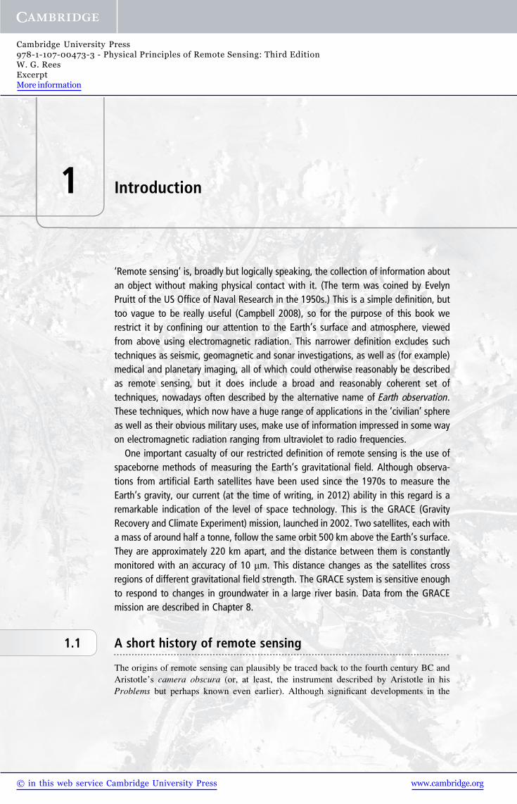
about 80 m. Tournachon, born in 1820, used the pseudonym ‘Nadar’ and was one of the
earliest developers of photography as art (Figure 1.1). He was also the inventor of the
crowd control barrier. Kites were also soon used, and by 1890 the usefulness of aerial
photography was so far recognised that Arthur Batut had published a textbook on the
subject (Batut 1890) (Figure 1.2).
Figure 1.1. ‘Nadar raising Photography to the level of Art’. Lithograph by Honore
Daumier, 1863. (Source: Brooklyn Museum, via Wikipedia. http://en.wikipedia.org/wiki/
Nadar_(photographer))
2 Introduction
Cambridge University Press978-1-107-00473-3 - Physical Principles of Remote Sensing: Third EditionW. G. ReesExcerptMore information
www.cambridge.org© in this web service Cambridge University Press

The next step towards what we now recognise as remote sensing was taken with the
development of practicable aeroplanes in the early twentieth century. Again, the potential
applications were quickly recognised and aerial photographs were recorded from aero-
planes from 1909. Airborne photography was used during the First World War for
military reconnaissance, and during the period between the two World Wars civilian uses
of this technique began to be developed, notably in cartography, geology, agriculture and
forestry. Cameras, film and aircraft underwent significant improvements, and stereo-
graphic mapping attained an advanced state of development. The modern descendants
of these applications are discussed in Chapter 5. Also during this period, John Logie
Baird, the inventor of television, performed early work on the development of airborne
scanning systems capable of transmitting images to the ground. This work (its modern
developments are discussed in Chapter 6) was highly confidential, having been carried out
on behalf of the French Air Ministry. It was ended by the war and forgotten about until
1985 (Burns 2000).
The Second World War brought substantial developments to remote sensing.
Photographic reconnaissance reached a high state of development – the German
invasion of Britain, planned for September 1940, was forestalled by the observation
of concentrations of ships along the English Channel. Infrared-sensitive instruments
and radar systems were developed. In particular, the Plan Position Indicator used by
night bombers was an imaging radar that presented the operator with a ‘map’ of the
terrain, and thus represented the ancestor of the imaging radar systems discussed in
Chapter 9.
By the 1950s, false-colour infrared film, originally developed for military use, was
finding applications in vegetation mapping, and high resolution imaging radars were
being developed. As these developments continued through the 1960s, sensors began to
be placed in space. This was originally part of the programme to observe the Moon, but
the advantages of applying the same techniques to observation of the Earth were soon
recognised, and the first multispectral spaceborne imagery of the Earth was acquired from
Figure 1.2. Labruguiere, photographed from a kite by Arthur Batut in 1889. (Source:
Wikipedia. http://en.wikipedia.org/wiki/Arthur_Batut)
3 1.1 A short history of remote sensing
Cambridge University Press978-1-107-00473-3 - Physical Principles of Remote Sensing: Third EditionW. G. ReesExcerptMore information
www.cambridge.org© in this web service Cambridge University Press
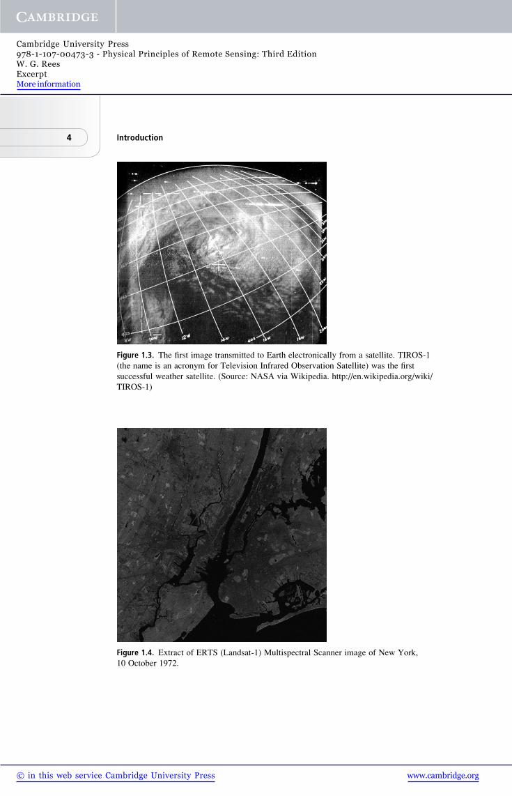
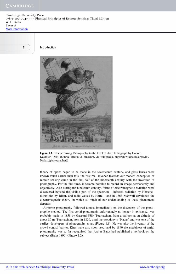
Figure 1.3. The first image transmitted to Earth electronically from a satellite. TIROS-1
(the name is an acronym for Television Infrared Observation Satellite) was the first
successful weather satellite. (Source: NASA via Wikipedia. http://en.wikipedia.org/wiki/
TIROS-1)
Figure 1.4. Extract of ERTS (Landsat-1) Multispectral Scanner image of New York,
10 October 1972.
4 Introduction
Cambridge University Press978-1-107-00473-3 - Physical Principles of Remote Sensing: Third EditionW. G. ReesExcerptMore information
www.cambridge.org© in this web service Cambridge University Press

Apollo 6. Although there were earlier unmanned remote sensing satellites (Figure 1.3),
the opening of the modern era of spaceborne remote sensing ought probably to be dated to
July 1972 with the successful operation of ERTS, the Earth Resources Technology
Satellite, by the US National Aeronautics and Space Administration (NASA) (Figure 1.4).
ERTS was renamed Landsat-1, and the Landsat programme is still continuing – at the
time of writing (2012), Landsat-5 and Landsat-7 were both still operational.
Since the launch of ERTS in 1972, the number and diversity of spaceborne and airborne
remote sensing systems has grown dramatically. A larger range of variables can be
measured, and consistent and systematic datasets can be constructed for progressively
longer periods of time. The explosive growth in the quantity of data being generated has
been matched by growth in the availability of computing resources and the facilities for
data storage and transmission. Since 2005, the availability of the Google Earth program
has greatly increased public exposure to and use of remote sensing data.
1.2 Applications of remote sensing................................................................................................................The enormous growth in the availability of remotely sensed data over the last four decades
has been matched by a fall in the real cost of the data. Nevertheless, it is still clear that use of
the data must offer some tangible advantages to justify the cost of acquiring and analysing
them. These advantages derive from a number of characteristics of remote sensing. Probably
the most important of these is that data can be gathered from a large area of the Earth’s
surface, or a large volume of the atmosphere, in a short space of time, so that a virtually
instantaneous ‘snapshot’ can be obtained. For example, scanners carried on geostationary
meteorological satellites such as METEOSAT can acquire an image of approximately one-
quarter of the Earth’s surface in less than half an hour.When this aspect is combined with the
fact that airborne or spaceborne systems can acquire data from locations that would be
difficult (slow, expensive, dangerous, politically inconvenient . . .) to measure in situ, the
potential power of remote sensing becomes apparent. Of course, further advantages derive
from the fact that most remote sensing systems generate calibrated digital data that can be fed
straight into and analysed by a computer.
Remote sensing finds a very wide range of applications, naturally including the area of
military reconnaissance in which many of the techniques had their origins. In the non-
military sphere, most applications can loosely be categorised as ‘environmental’, and we
can distinguish a range of environmental variables that can be measured. In the atmosphere,
these include temperature, precipitation, the distribution and type of clouds, wind velocities,
and the concentrations of gases such as water vapour, carbon dioxide, ozone etc. Over land
surfaces, we can measure tectonic motion, topography, temperature, albedo (reflectance)
and soil moisture content, and determine the nature of the land cover in considerable detail,
for example by characterising the type of vegetation and its state of health or by mapping
man-made features such as roads and towns. Over ocean surfaces, we can measure the
temperature, topography (from which the Earth’s gravitational field, as well as ocean tides
and currents, can be inferred), wind velocity, wave energy spectra and colour (which is
often related to biological productivity by plankton). The ‘cryosphere’, that part of the
Earth’s surface covered by snow and ice, can also be studied, giving data on the distribution,
condition and dynamical behaviour of snow, sea ice, icebergs, glaciers and ice sheets.
5 1.2 Applications of remote sensing
Cambridge University Press978-1-107-00473-3 - Physical Principles of Remote Sensing: Third EditionW. G. ReesExcerptMore information
www.cambridge.org© in this web service Cambridge University Press

This list of measurable variables, while not complete, is large enough to indicate that
there is a correspondingly large number of disciplines to which remote sensing data can
be applied. While by no means exhaustive, a list of applications could include the
following disciplines: agriculture and crop monitoring, archaeology, bathymetry, cartog-
raphy, civil engineering, climatology, coastal erosion, disaster monitoring and prediction,
forestry, geology, geomorphology, glaciology, meteorology, oceanography, pollution
monitoring, snow resources, soil characterisation, urban mapping, and water resource
mapping and monitoring. It is not really possible to present a detailed cost–benefit
analysis in this introduction. The development, insertion into orbit, and operation of a
large remote sensing satellite costs typically a couple of billion euros. Perhaps it is
sufficient to point out that the data available from remote sensing, particularly from
spaceborne observations, can often not be obtained in any other way, that our current
understanding of the global climate system is very largely based on spaceborne observa-
tions, and that the use of remotely sensed data for disaster warning has already saved
many thousands of human lives.
As implied in Section 1.1, the era of systematic observation of the Earth from space is
approaching middle age when seen from the perspective of a human lifespan. Landsat
images have been collected continuously for over 40 years, radar altimeter data (which
can be used to study changes in sea level, amongst many other applications) have been
collected for over 20 years, and other examples can easily be found. These time-scales are
long enough to form the basis of increasingly reliable measurements of change in many
areas, not least of which is global change.
1.3 A systems view of remote sensing. . . . . . . . . . . . . . . . . . . . . . . . . . . . . . . . . . . . . . . . . . . . . . . . . . . . . . . . . . . . . . . . . . . . . . . . . . . . . . . .We stated above, rather briefly, that remote sensing involves the collection of infor-
mation, carried by electromagnetic radiation, about the Earth’s surface or atmosphere. Let
us try to expand this statement a little.
First, where does the radiation come from? One major classification of remote sensing
systems is into the passive systems, which detect naturally occurring radiation, and the
active systems, which emit radiation and analyse what is sent back to them. The passive
systems can be further subdivided into those that detect radiation emitted by the Sun (this
radiation consists mostly of ultraviolet, visible and near-infrared radiation), and those that
detect the thermal radiation that is emitted by all objects that are not at absolute zero (i.e.
all objects). For objects at typical terrestrial temperatures, this thermal emission occurs
mostly in the infrared part of the spectrum, at wavelengths of the order of 10 mm (the so-
called thermal infrared region), although measurable quantities of radiation also occur at
longer wavelengths, as far as the microwave part of the spectrum. Active systems can, in
principle, use any type of electromagnetic radiation. In practice, however, they are
restricted by the transparency of the Earth’s atmosphere. This is shown schematically in
Figure 1.5. Chapter 4 presents a detailed discussion of the interaction of electromagnetic
radiation with the atmosphere.
Figure 1.5 shows that there are three main ‘windows’ in the atmosphere. The first of
these includes the visible and near-infrared (VNIR) parts of the spectrum, between
wavelengths of about 0.3 mm and 3 mm, although it does also contain a number of opaque
6 Introduction
Cambridge University Press978-1-107-00473-3 - Physical Principles of Remote Sensing: Third EditionW. G. ReesExcerptMore information
www.cambridge.org© in this web service Cambridge University Press

regions. The second is a rather narrow region between about 8 mm and 15 mm, in which is
found the bulk of the thermal infrared (TIR) radiation from objects at typical terrestrial
temperatures. The third more or less corresponds to the microwave region, between
wavelengths of a few millimetres and a few metres. Thus we can expect that any active
system designed to penetrate the Earth’s atmosphere will operate in one of these three
‘window’ regions.
Table 1.1 summarises the main types of remote sensing system on the basis of the
classifications we have just outlined. Sounding instruments, intended to profile some
property of the atmosphere such as its temperature or chemical composition, generally
operate on the boundaries between transparency and opacity of the atmosphere.
The sensor, whether it is part of a passive or an active instrument, detects electromag-
netic radiation after it has interacted with or been emitted by the ‘target’ material. In what
way can this radiation contain useful information about the target? There are essentially
only two variables to describe the radiation that is received: how much radiation is
detected (we may need to qualify this with a statement about the polarisation of the
radiation), and when does it arrive? The time-structure of the detected radiation is
obviously only relevant in the case of active systems where the time-structure of the
emitted radiation can be controlled. In this case it is possible to determine the distance
from the sensor to the target, and this is the principle behind various ranging systems such
as the laser profiler, LiDAR, radar altimeter and other types of radar system. In all other
Figure 1.5. Transparency of the Earth’s atmosphere as a function of wavelength (schematic).
Black regions are opaque, white regions transparent.
Table 1.1. A simple taxonomy of remote sensing systems, excluding sounding instruments.The numbers in parentheses refer to the chapters of this book.
Active systems
Passive systems Ranging Imaging
VNIR Aerial photography (5)
Electro-optical systems (6)
Laser profiler (8)
TIR TIR imager (6)
Microwave Passive microwave
radiometer (7)
Radar altimeter (8)
Ground-penetrating
radar (8)
Microwave
scatterometer (9)
Imaging radar (9)
7 1.3 A systems view of remote sensing
Cambridge University Press978-1-107-00473-3 - Physical Principles of Remote Sensing: Third EditionW. G. ReesExcerptMore information
www.cambridge.org© in this web service Cambridge University Press

cases, the only information we have is the quantity of radiation received at the sensor. If
the radiation arises from thermal emission, the quantity is characteristic of the tempera-
ture of the target material and its emissivity, a property that describes its efficiency at
emitting thermal radiation. Otherwise (in the cases of both passive and active systems that
measure reflected radiation) the amount of radiation that is received is determined by the
amount illuminating the target material, and the target’s reflectivity. Thus we can see that
the information about a target material that is directly observable from remote sensing
observations is actually rather limited: we can measure its range, its reflectivity, and a
combination of its temperature and emissivity. However, these can be measured at
different times, over a range of wavelengths and, sometimes, in different polarisation
states, and this increase in the diversity of the variables at our disposal is responsible for
the large range of indirect observables that was sketched out in Section 1.2.
The foregoing discussion has not included the effects of the Earth’s atmosphere,
except to point out that atmospheric opacity limits the scope for observing the Earth’s
surface to the main atmospheric ‘windows’. In fact, as almost any electromagnetic wave
propagates through the atmosphere, its characteristics will be somewhat modified. This
modification may be troublesome, requiring correction, or advantageous depending on
whether we are more interested in studying the Earth’s surface or the atmosphere itself.
In general, we can say that if the observation is made at a wavelength at which the
atmosphere is opaque, the measured signal will be characteristic of the atmosphere,
whereas if the atmosphere is transparent, the data will be characteristic of the surface
below.
Once the data have been collected by the sensor, they must be retrieved and analysed.
In many, though not all, cases, the data will form an image, by which we mean a two-
dimensional representation of the two-dimensional distribution of radiation intensity.
Since the second edition of this book appeared in 2001, the concepts of digital imaging
and digital images have become much more generally familiar as a result of the huge
increase in the popularity of digital photography and the use of Google Earth and similar
web-based resources. The images with which we have to deal in remote sensing are
normally digital, so they can conveniently be analysed by computer, and need not be
confined to the visible part of the electromagnetic spectrum. For example, an image might
represent the radar reflectivity in one or more frequencies or polarisation states, or the
thermal emission, as well as the visible or near-infrared reflectivity. Image processing
forms an integral part of remote sensing. Typically, this involves several steps. The first is
to correct the image so that it has a known geometrical correspondence to the Earth’s
surface and a known calibration, with atmospheric propagation effects removed. At this
stage, the image may also be enhanced in various ways, for example by suppressing noise,
to increase its intelligibility. The major goal of image processing, however, is the
extraction of useful information from the sensor data, based on the brightness values of
the image (probably in a number of spectral bands, at a number of different dates, in
different polarisation states etc.) and also on the spatial context. Using the analogy of a
colour photograph, we can say that information can be extracted on the basis of colour,
texture, shape and spatial context. In the majority of cases, it is necessary or at least
desirable to ‘train’ the process of extracting information from the image using data from
known locations. The process can therefore be seen as one of extrapolation from areas that
are already known, for example on the basis of field work, to much wider areas. The
8 Introduction
Cambridge University Press978-1-107-00473-3 - Physical Principles of Remote Sensing: Third EditionW. G. ReesExcerptMore information
www.cambridge.org© in this web service Cambridge University Press

extrapolation need not be confined to the spatial domain, however, and the analysis of
time-series of images for change detection is also an important application of remote
sensing.
1.4 Further reading, and how to obtain data................................................................................................................The field of remote sensing is now well served with textbooks, and the interested (or
puzzled) reader should be able to find alternative treatments of most of the topics
discussed in this book. While what follows is a personal list and makes no pretence to
completeness, recent general textbooks include the fourth edition of Campbell’s Intro-duction to Remote Sensing (Campbell 2008) and the sixth edition of Lillesand, Kiefer and
Chipman’s Remote Sensing and Image Interpretation (Lillesand, Kiefer and Chipman
2008), while the SAGE Handbook of Remote Sensing (Warner, Nellis and Foody 2009)
provides exceptional breadth of treatment. Somewhat more detailed or more specialised
treatments are given by, for example, the second edition of Jensen’s Remote Sensing of
the Environment (Jensen 2006), Jones and Vaughan’s Remote Sensing of Vegetation(Jones and Vaughan 2010), Purkis and Klemas’s Remote Sensing and Global Environ-
mental Change (Purkis and Klemas 2011), Liang’s Quantitative Remote Sensing of Land
Surfaces (Liang 2004) and the second edition of Elachi and van Zyl’s Introduction to thePhysics and Techniques of Remote Sensing (Elachi and van Zyl 2006).
Scientific journals also represent an important source of information. Articles in the
scientific literature are usually aimed at specialists, but the more general reader can often
also extract a useful understanding from them, and the journals sometimes also publish
review articles. In this book I have provided references to both books and journal articles.
The principal English language journals in remote sensing are the Canadian Journal ofRemote Sensing, Computers & Geosciences, Geophysical Research Letters, IEEE Trans-
actions on Geoscience and Remote Sensing, the International Journal of Remote Sensing,
Photogrammetric Engineering and Remote Sensing, and Remote Sensing of Environment.Finally, a few remarks about the Internet may be useful. This can represent a very
powerful means of obtaining up-to-date information of all sorts, for example on the
operational status of a particular remote sensing satellite, or the latest results from a
research group, or access to remote sensing data (indeed, some of the illustrations used in
this book have been obtained in this way) or the software needed to process it. As anyone
who has grappled with the Internet will know only too well, the problem is usually to
locate the information one needs. The well-known search engines can be extremely
helpful, as can the collections of links assembled by public-spirited individuals and
organisations. The website of this book is located at www.cambridge.org/
9781107004733 and it includes a collection of links to some other useful websites
including online catalogues from which satellite data may be located.
A question that inevitably arises when one starts to consider obtaining satellite or other
remotely sensed imagery is – what does it cost? There is no single, simple answer to this
question. As a rough guide, though, one may say that the coarser the spatial resolution of
the imagery the more likely it is to be freely available, and the finer the spatial resolution
the more likely it is to be rather expensive, by which one might mean a thousand pounds
or equivalent. As an example, imagery from a particular commercial spaceborne
9 1.4 Further reading, and how to obtain data
Cambridge University Press978-1-107-00473-3 - Physical Principles of Remote Sensing: Third EditionW. G. ReesExcerptMore information
www.cambridge.org© in this web service Cambridge University Press
instrument, having a spatial resolution of around 1m, cost US$10–20 per square kilo-
metre in late 2010, while MODIS imagery, with a spatial resolution of 250–1000 m, was
freely available. Images collected by the Landsat series of satellites, having spatial
resolutions of 15–80 m, were also freely available at the time of writing. The trend over
the last decade or so has been towards the free availability of satellite imagery.
As noted in Section 1.3, quantitative processing of spatial data is an integral part of
remote sensing. Some of the mathematical principles of image processing are discussed in
Chapter 11. There is of course a wide range of computer software for manipulating and
processing image data, often very powerful and flexible. However, such software can also
manifest some disadvantages. It may be expensive, demanding of computing resources
(memory, processing power and so on), able to run only on specific computing platforms,
dependent on its own specific file formats, and so on. In contrast to this approach is the
existence of free software, especially when developed in an open-source environment.
The website of this book has links to sources of free software for image processing and for
geographic information systems (GIS), a related technology that is discussed briefly in
Chapter 11. In addition, readers of this book might wish to develop their own software for
carrying out image processing operations. Again, there are several suitable possibilities
among programming languages. Of freely available programming languages, two of the
most useful are R and GNU Octave, both available since the early 1990s. GNU Octave is
designed particularly for manipulating matrices, and since images share many properties
with matrices (see Chapter 11) it is particularly well suited to processing images. GNU
Octave runs under most computer operating systems. The book’s website has a number of
Octave programs that the reader can download and use to explore some of the topics
discussed in the text, and readers are encouraged to submit their own programs.
10 Introduction
Cambridge University Press978-1-107-00473-3 - Physical Principles of Remote Sensing: Third EditionW. G. ReesExcerptMore information
www.cambridge.org© in this web service Cambridge University Press