1. INTRODUCTION

The present investigation of long slender cylinders in axial and near axial flow

was motivated by the current interest in the fluid flow over towed sonar arrays. Such

arrays are used to locate and identify underwater vehicles by the analysis of sound

recordings obtained from the hydrophones (underwater microphones) in the array.

Means are needed by which the fluid flow over the sleeve containing the microphones

and associated cables may be analysed to improve the discrimination between the noise

generated by the movement of the microphone array itself and that generated by distant

underwater vehicles or other noise sources.

The problem in terms of fluid mechanics is to describe the fluid flow over long

circular cylinders in both axial flow and at small angles of yaw, with the intention of

identifying any larger scale flow processes in either the cylinder boundary layer, or in

the wake therefrom, which occur at frequencies lower than that of the fine scale

turbulence (of order 10 kHz). Regular periodic processes are of particular interest. This

requires an extension of the current understanding of cylinder wakes to include very

small yaw angles, and an extension of the current understanding of turbulent boundary

layers to include cases of very long cylinders in axial and near axial flow.

On the basis of results obtained in their experimental investigation of thick

turbulent boundary layers on very long cylinders in axial flow, Luxton et al. (1984)

suggested that the stripping of retarded inner-layer fluid from the cylinder by turbulent

cross-flows, accompanied by the generation of high instantaneous velocity gradients at

the cylinder surface, could be responsible for the high levels of vorticity production

L

necessary for the small cylindrical surface area to sustain the large volume of

turbulence surrounding it. This volume of turbulence, per unit of surface area, may be

an order of magnitude or more greater than that in a flat-plate boundary layer. The

requirement for higher levels of vorticity production in a thick axisymmetric turbulent

boundary layer than in a flat-plate layer also leads to the expectation of higher wall

shear stresses in the axisymmetric case, and experimental results such as those of

Willmarth and Yang (1970), Willmarth et.al.(1976), Lueptow et.al.(1985), Lueptow

and Haritonidis (1987), and Cipolla and Keith (2003a, 2003b) are in accord with this

expectation.

In later work by Bull et al.(1988), additional support for this hypothesis came

with preliminary evidence suggesting the existence of propagating fronts of low speed

fluid in the boundary layer. This, in turn, raised the possibility that stripping of

retarded fluid from the cylinder might be associated with localised vortex shedding

being induced by turbulent cross-flows.

The effects of such cross-flows have been interpreted by Lueptow and

Haritonidis (1987) in terms of the burst-sweep mechanism of turbulence generation

identified in planar boundary layers, with modification for transverse curvature. It is

proposed here that the cross-flow effects in the boundary layer on a slender cylinder in

axial and near-axial flow constitute a different, and possibly dominant, turbulence

generation mechanism from that characterising planar boundary layers. As a

consequence, an investigation was undertaken of vortex shedding from cylinders yawed

at small angles from the flow direction, and of the turbulence mechanisms within the

axisymmetric boundary layer formed at zerc yaw.

J

The investigation of vortex shedding from a yawed cylinder is to determine the

Reynolds-number and yaw-angle regimes where vortex shedding occurs, and to

determine the frequency f and orientation o of the vortices as a function of the cylinder

geometry and the flow state. The cylinder geometry is defined by the three variables:

diameter d, location x along the overall length /, and yaw angle p.

The flow state is defined by three parameters, the free stream velocity U,, the

fluid density p and the fluid viscosity pr,. Thus the overall condition of the flow over a

cylinder shedding vortices at an angle o, and a frequency f may be described by the set

of variables { d, X, 0, Ur, p, F, a, f }. For a particular cylinder i fluid combination,

experiments have been performed to measure the vortex shedding frequency and

orientation while the flow velocity and yaw angle are varied to obtain a relationship of

the form:

These dimensional forms may be generalised to collapse data from a variety of

cylinder-geometry / fluid-velocity combinations by forming non-dimensional parameters

from f, U,, 0 and x. The velocity U, is non-dimensionalised as a Reynolds number

f : function( U,, 0, x ),

a : function( U,, 0, x ).

Reo: pUrdlp : Urd lv

or Rgu : pUralp : Uralv ,

[ 1 . 1 a ]

[ 1 . 1 b ]

lr.2l

based on diameter or radius, and the periodic vortex shedding frequency may be non-

dimensionalised as

F : pfdzlp : fdzlv . t1 .31

4

An alternative to the non-dimensional frequency parameter F is the Strouhal

number St, where St : F/Rea : fdlUr. Although the use of Strouhal number is more

common, the use of F allows the effects of frequency and flow velocity to be

separated.

The yaw angle is itself non-dimensional, but may also be expressed as a

trigonometric function such as sin 0, which may be interpreted physically as the ratio

of the cross-flow velocity component to the total free stream velocity. The orientation

of the vortex line to the cylinder axis a is also non-dimensional, and expresses the ratio

of the axial to normal vorticity generated by the cylinder. The length x may be non-

dimensionalised as the length-to-radius ratio xla, a measure of the "slenderness" of the

cylinder, or as a Reynolds number based on length:

R e * : p U r x l p : U r x l u u.4l

Thus the formal relationships, in terms of non-dimensional parameters, are

F _

a n d d :

function( B, Reo, x/a )

function( 0, Reo, xla).

[1 .5 a ]

[ 1 . 5 b ]

The non-dimensional frequency F can be expected to vary with x/a as the

thickness of the cylinder boundary layer increases (implying that vortex cells are

formed in the flow), an effect which will decrease as the yaw angle increases. In the

extreme case of 0 : 90" the axial velocity component approaches zero and the flow

becomes independent of x. For the small yaw angles and very large xla considered

here, the flow is only weakly dependent on x/a as the axial flow is well developed.

5

Similarity analysis of the mean flow within planar turbulent boundary layers

(Coles 1955,1956,1957) indicates the presence of inner and outer layer regimes. The

inner layer regime is scaled on the friction velocity U", defined in terms of the wall

shear stress as U" : t[(r*lp). The normalised local non-dimensional velocity and

distance from the wall are then expressed in "wall units" as U* : U/U" and

,+ : yU,lz respectively. The outer layer regime is scaled on the free stream velocity

U1 and the boundary layer thickness 6. Thus the non-dimensional parameters for

velocity and position in this region are U/U, and y/6 respectively.

The addition of the transverse curvature, characterised by the cylinder radius a,

for the axisymmetric boundary layer introduces two new non-dimensional parameters.

These are the ratios of the length scales of each of the inner and the outer layers to the

radius of transverse curvature. Thus for the inner layer length scale, vlU,, the ratio

becomes vlaU,, that is 1/a*, where a* : aU,lv, and for the outer length scale 6 the

ratio becomes 6/a.

The investigation of the effects of transverse curvature on the mechanisms of

turbulence production within the thick axisymmetric boundary layer formed at zero yaw

angle (6 : 0") examines the case where the curvature is large in comparison with both

the inner and outer length scales. This requires small a* and large 6la. As a+ is

proportional to Re" (Luxton et.a1.1984) and 6 increases with x, this means small Re"

and large x/a. The investigation demonstrates the occurrence of cross flows of

boundary layer fluid over the cylinder, which result in fluid being removed from the

inner regions of the boundary layer to form fronts of low speed fluid which extend

across the boundary layer radius. This process is found to be repeated continuously but

aperiodically.

6

The form of this axisymmetric boundary layer may be described by the

momentum integral equation (Equation t1.61 below) which is obtained by the

integration of the equation of motion of the boundary layer from the cylinder surface to

the outer edge of the boundary layer.

The momentum integral equation is expressed in terms of a momentum

thickness 0, (Equation [1.7] below), and a displacement thickness 6r. (Equation [1.8]

below) as

( 1 +0, d0, I- l - +

; ' d x u ,dU. 0^ r' 0- (l + --! \ (H-*2\ = *d x z ' 2 a " z

p u i

where

( o r * a ) t - a t#, )2rdr

t 1.61

Ir.7l

(6; * a)'

and

#, )Zrdr

="lt['

-o ' = ' i u [ ' l l . 8 l

H r =

0,0.*)

Equation [1.6] shows that d9rldx will be positive for a non-zero wall shear

stress r* and zero pressure gradient (ie. dU,/dx : 0); thus the boundary-layer thickness

will continue to increase with increasing values of x. For the current experiments at

I

xla : 6000, the ratio of boundary layer thickness to cylinder radius 6la can be as high

as 50. The results of Luxton et al.(1984) show that for boundary layers with Re, in the

range 1000 - 3000 and Reu and a* as low as 140 and 13 respectively the layer is fully

turbulent. They show, further, that, as xla becomes large (xla > 5000, 6/a > > 1),

the shape of the axisymmetric boundary layer approaches a state of similarity and the

rate of boundary-layer growth becomes very small. The current experiments, conducted

at xla : 6000 with 2000 ( Reu, < 3000, Re" in the range 300 - 600 and a* in the

range 22 - 41, can therefore safely be assumed to be representative of the fully-

developed boundary layer in its asymptotic form.

l..1 Aims of the Research Program.

The aim of the research program is to advance the current understanding of the

flow processes characterising a long slender cylinder in axial and near axial flow. As

described in the following chapters, this is achieved by an experimental investigation of

the flow by means of velocity measurement and flow visualisation. In the axial flow

case, the resultant thick axisymmetric turbulent boundary layer is examined to

determine both the mean and statistical properties of the turbulent flow. From these

measurements the characteristics of the boundary layer are compared with the well

established case of the flat plate boundary layer, and also with the axisymmetric

boundary layer with smaller 6/a, which is the subject of current research by other

investigators, (see, for example, Bokde, Lueptow and Abraham 1999).

Further investigation of the axisymmetric boundary layer to determine the

character of the fronts of low speed fluid, thought to be associated with large negative

spikes observed in the time series records of the turbulent velocity fluctuations. is

described. Experiments to determine the flow mechanism by which these fronts are

formed are discussed, and a description of the associated turbulence generation process

is formulated to explain how, and why, this type of boundary layer differs from both

the flat plate and the small 6/a axial-cylinder cases.

For the near axial flow case, the asymmetry of the turbulent boundary layer has

been measured for very small yaw angles in order to determine the geometric limits

within which the prior results for the axisymmetric boundary layer may reasonably be

9

applied. For larger yaw angles, greater than one degree, the occurrence of regular

vortex shedding is examined. The regime of flow within which regular vortex shedding

occurs is determined, and measurements of the vortex shedding frequency within this

regime are presented. From these measurements the characteristic relationship between

the vortex shedding frequency, the cylinder geometry and the properties of the fluid

flow is determined in terms of non-dimensional parameters.

1 0

2. LITERATURE REVIEW

Previous research on circular cylinders in axial and near-axial flow has been

conducted in two major fields: the analysis of the boundary layer and mechanisms of

turbulence production, and the analysis of the vortex shedding behaviour.

The vast majority of the relevant boundary layer research seeks to modify flar

plate boundary layer theory to account for the effects of transverse curvature to provide

a description of the axisymmetric boundary layer generated on a cylinder for 6/a < 5.

The knowledge of mean boundary layer properties has been extended to account for the

effect of yawing the cylinder from the axial case. The mechanism of turbulence

production in such flat-plate and axisymmetric boundary layers has yet to be fully

understood, and is the subject of a large volume of current research. The effects of

increasing 6/a and possible cross-flows within the boundary layer on the mechanisms of

turbulence production in thick boundary layers have yet to be explained for 6/a > ) 1

for cylinders in axial and near-axial flow. Such considerations have stimulated the

present investigation of turbulence production in thick axisymmetric boundary layers.

Vortex shedding in the wake of cylinders which are orientated transversely to

the flow direction is well known. When the flow is other than normal to the cylinder

axis, the 'normal' vortex shedding theory must be modified to account for the effect of

yaw. While data on vortex shedding from near-normal cylinders abounds, no previous

research has been found to extend the yaw angle beyond 76' from the normal, which

corresponds to an angle relative to the cylinder axis of 0 : 14". At the other end of

1 1

the scale Luxton et.al.(1984), Lueptow et.al.(1985,1986,1987) and Cipolla and Keith

(2003a,2003b) have studied flows along slender cylinders aligned with the flow

direction. The present experimental investigation seeks to 'close the gap' between these

two families of experiments by studying the vortex shedding from cylinders in near-

axial flow.

t2

2.1 Turbulent Boundary Lavers.

Initial methods to describe boundary layer turbulence were based on the

characterisation of flat-plate turbulent boundary layers in terms of the flow parameters

and the production and dissipation of energy within the layer. Townsend (1956)

provides the basis for this analysis by considering the boundary layer to be composed

of two distinct parts, an inner layer wholly controlled by the local wall stress, and an

outer layer with wake-like properties. Analytical descriptions of the mean boundary

layer properties within these two regions have been developed by similarity analysis to

identify the relevant scaling parameters, and by the application of the concepts of "the

law of the wall" [Coles(1955)] for the inner region, and "the law of the wake"

[Coles(1956,1957)l for the outer region. Early analytical models of the structure of

turbulence by Theodorsen (1952, 1955) identify the "horseshoe" vortex, and a series of

smaller "horseshoe" vortices formed over the surface of the primary vortex, as the

principal coherent structures within a turbulent boundary layer. The further analysis of

the fundamental mechanisms by which these turbulence processes occur has progressed

largely by experimental investigations spanning the whole class of shear flows.

Correlation measurements of fluctuating velocities and wall pressures by

Wooldridge and Willmarth (1962) lead to their hypothesis that the measured vector

field of the pressure-velocity correlation data can be represented by a velocity field

generated by the superposition of a spectrum of eddies whose axes are perpendicular to

the mean velocity, in a plane parallel to the wall, which interfaces with a layer of fluid

near the wall. Flow visualisation studies by Kline et.al. (1967) reveal the presence of

13

low speed streaks in the near-wall region. These were observed to interact with the

outer layer by a process of gradual 'lift-up', followed by sudden oscillation, bursting,

and ejection, leading to the hypothesis that these processes are an important mechanism

in the generation and transport of turbulence within the boundary layer.

Visual investigations by Corino and Brodkey (1969) of pipe flow boundary

layers also detected the ejection of fluid elements from the wall region, and identified

the interaction of this process with the mean flow as an important factor in the creation

of turbulence. The initial analysis of the frequency of these inner-layer events, termed

'bursts' by Rao et.al. (1971) and by Laufer and Narayanan (1971), suggests that the

mean frequency of the bursts scales with the outer-layer variables, and that the

mechanism can thus best be explained in terms of a coupling between the inner and

outer layers.

Further investigations of the wall region by Blackwelder and Kaplan (1976)

confirm that, although the bursting process has its largest effect near the wall and,

although its vertical extent scales on the inner-layer variables, its frequency of

occurrence scales on the outer-layer variables. However, further analysis of the

bursting frequency by Blackwelder and Haritonidis (1983) led to the conclusion that the

mean frequency really scales with the inner-region variables. These authors attributed

the previous findings of outer-region scaling to the effects of spatial averaging over the

sensor length. Subsequent examinations by Alfredsson and Johansson (1984 a) found

that the governing time scale for events in the near-wall region is a mixture of both

inner and outer time scales. The work of Wark and Nagib (1991) indicates that a

hierarchy of burst-event sizes exists. They suggest that the time scales are generated by

l 4

a wall-layer mechanism but grow to scales and are convected with velocities determined

bv the outer laver.

The relative importance of these burst events in the production of turbulence has

been determined by Willmarth and Lu (1972) by conditional sampling of the u and y

velocity components. These measurements indicate that the contribution of the bursting

process to the Reynolds stress and to the turbulent energy production in the near-wall

region occurs intermittently, and is of relatively large magnitude and of short duration.

Flow visualisation of the bursting process by Nychas et.al. (1973) confirms the

importance of the process in the production of turbulence and additionally shows that

the recovery process, termed "sweeps", also makes positive contributions to the

Reynolds stress. A model of the burst-sweep process was proposed by Offen and Kline

(1975) envisaging wallward "sweeps" of fluid, caused by large scale eddies, generating

pressure gradients that are sufficiently adverse to lift low speed streaks of fluid up from

the wall ("bursts"). New low speed streaks are then formed downstream by fluid

elements from the burst returning to the wall and being decelerated by viscous forces.

The process can loosely be described as a sequence of intermittent 'internal separations'

within the turbulent boundary layer.

The spanwise structure of the burst mechanism near the wall examined by

Blackwelder and Eckelmann (1917,1979) suggests the existence of a system of counter-

rotating streamwise vortices which are disturbed intermittently by high speed sweeps.

These streamwise vortices "pump" fluid away from the wall, thus forming low speed

streaks which are eventually terminated by a sweep. Measurements by Willmarth and

Bogar (1977) also support the proposition of streamwise vorticity as the mechanism for

15

producing intermittent small scale disturbances in the near wall flow. Ensemble

averages of the conditionally-sampled turbulent velocity fluctuations by Wallace et.al.

(1917) show a characteristic gradual deceleration of the u component followed by a

strong acceleration, in agreement with the burst-sweep model.

Analysis of the large scale outer layer structures by Thomas (1977), Brown and

Thomas (1971) and Thomas and Bull (1983), suggests the existence of organised

structures on the scale of the full boundary layer, in the form of oblique fronts of fluid

which they postulated to be the initiators of the wall region events. A visual study of

such coherent structures by Praturi and Brodkey (1978) supports this concept of the

outer-layer structure driving the inner-layer events. Further evidence for the formation

of oblique fronts is provided by Kreplin and Eckelmann (1979), who postulate that the

fronts originate from the inclined streamwise vortices. The spanwise structure of the

bursts and sweeps measured by Antonia and Bisset (1990) indicates that the sweeps are

approximately 25% wider than the bursts, and are twice as long in the streamwise

direction.

An examination by Morrison et.al. (1992) of ejections and sweeps detected by

conditional sampling of experimental velocity data indicates that the interaction of the

inner and outer layers is controlled principally by the ejections from the inner layer.

The results of experimental emulation of turbulent-boundary-layer eddy structures,

conducted by Myose and Blackwelder (1994), indicate that the outer region of the

turbulent boundary layer also plays a role in the bursting process. The analysis of

numerical simulations of transitional and turbulent boundary layers by Rempfer and

Fasel (1994 a,b) suggest the possibility of determining the structure of turbulence as a

1 6

non-linear interaction, perhaps involving only a small number of coherent structures.

The merits of the various sampling and averaging techniques used in detecting

turbulent structures are compared by Subramanian et.al. (1982) with the conclusion that

multiple point rake detection schemes are preferable to single point measurement

methods. The addition of pattern recognition to single point detection schemes by

Blackwelder (1977) increases the effectiveness of simple conditional sampling

techniques by suppressing the effects of the random phase which occurs between

spatially or temporally separated signals. Zaric's (1982) method of pattern recognition

however improves the single point method to a similar level by using a more complex

event detection scheme based on the separate detection of both a burst and a sweep

rather than detection of a complete sweep pattern. The merit of this method is also

demonstrated by combined flow visualisation and hot-wire anemometry analysis of the

flow by Zaric et.al. (1984). The advantages of combined flow visualisation and

anemometry are further demonstrated by Wei et.al. (1984) in examining individual

large scale events without the possible loss of information resulting from any averaging

process.

A comparison by Alfredsson and Johansson (1984 b) of the uv-quadrant method

of analysis with the variable interval time averaging (VITA) technique suggests that

similar results may be obtained by both methods provided that suitable VITA detection

criteria are used. A more extensive comparison by Bogard and Tiederman (1986) of

various detection schemes and flow visualisation results found that the quadrant

technique provides the greatest reliability, and provides a high probability of detecting

fluid ejections and a low probability of recording false detections. In Nagano and

I 7

Tagawa's (1995) study the u,v quadrant scheme has been further developed into a

trajectory analysis technique (TRAT) designed to evaluate a fluid motion (turbulence

structure) rather than to detect events only.

Various mechanisms have been advanced to explain the overall burst-sweep

process. Falco (1982, 1983), proposed a turbulence model based on a vortex ring

formed in the outer layer, which then approaches the wall at an acute angle. Initially

behaving as a three-dimensional sweep, the ring appears as two upwardly inclined

streamwise vortices as it interacts with the wall, producing the burst of ejected inner

layer fluid. Smith and Metzler (1983) examined the formation and origin of 'stretched

vortex loops', also referred to as'hairpin vortices', as a mechanism for the formation

of low speed streaks. This mechanism of vortex stretching as a source of turbulence

production is also supported by the theoretical analysis by Coles (1984).

Theoretical models for near-wall turbulence are proposed by Haritonidis (1989),

based on a modified mixing length hypothesis, and by Landahl (1990), based on a

quasi-laminar model. These determine the characteristics of the turbulence resulting

from a given burst geometry. The origin of the bursts suggested by Landahl (1990) lies

in the formation of the streaky structure in the sub-layer. Such streaks grow from any

initial local three-dimensional disturbances that have a non-zero net vertical momentum

along lines of constant !,2 (Landahl 1980). These disturbances could be initiated by any

local inflectional instability region with spanwise asymmetry, such as an oblique wave-

like disturbance which may result from a cross-flow instability induced by a large-scale

spanwise motion (Landahl 1975). A theoretical model for the distribution of streamwise

turbulence intensity has been formulated by Marusic et.al.(1997) based on the attached-

l 8

eddy model developed by Perry and Marusic (1995) and Marusic and Perry (1995).

The currently unsolved central issues in 'understanding' coherent boundary-layer

motions are identified by Robinson (1991) as (a) vortex formation and evolution, and

(b) interaction between coherent motions in the inner and outer regions of the boundary

layer. Any model of coherent structures in the turbulent boundary layer must address

both of these points, and also the Reynolds number dependence of the mechanisms

involved, if it is to be generally applicable. Such a model has been suggested by Falco

(1991) following a review of the many coherent motions detected previously, and

consequent formulation of a proposed interaction mechanism and its Reynolds number

dependence.

The successful identification of the attached vortex loops, envisaged by

Theodorsen (1955), within the numerically simulated data for a flat plate turbulent

boundary layer by Chong et.al.(1998), indicates that future studies of coherent

structures within boundary layer turbulence may be conducted with some reliability by

examining numerically-generated data.

The successful application of hydrogen-bubble flow-visualisation to the

investigation of near-wall streamwise vortices and the associated fluid ejections in a flat

plate boundary layer with mild streamwise curvature by Flack (1991) indicates the

effectiveness of this technique for flat plate boundary layers with a simple three-

dimensional aspect. It also suggests that the technique may be useful in the further

study of coherent structures within turbulent boundary layers with stronger transverse

curvature.

t 9

2.2 Botndary Layers on Cylinders Aligned with the Flow.

The current research is concerned with the very thick turbulent layer and the

flow mechanisms which sustain it. Previous investigations have been conducted over a

large range of Reynolds number (Re^) and relative boundary layer thickness (d/a) for

both laminar and turbulent boundarv lavers.

Early analytical investigations of axisymmetric boundary layers by Seban and

Bond (1951), Kelly (1954), Glauert and Lighthi l l (1955) and Cooke (1957) were

restricted to the analysis of laminar flows. They produced results which described

axisymmetric laminar boundary layers in terms of thickness and mean velocity profiles.

The accuracy of these results has subsequently been improved by Curle (1980). This

early analytical work was extended by Eckert (1952) to include turbulent boundary

layers; however, the assumptions then made, in the absence of experimental results, on

the effects of transverse curvature are now recognised as being inadequate.

Experimental measurements of the mean turbulent boundary layer properties by

Richmond (1957), Yu (1958), Yasuhara (1959), Willmarth and Yang (1970) , Rao and

Keshaven (1912) and Afzal and Singh (1976), have been compiled by Luxton et.al.

(1984) by plotting the values of Reu against a* for each data set, and by noting the

corresponding values of 6/a and whether the velocity profile data match the inner-layer

characteristics (an identifiable logarithmic region in the velocity profile) of the two-

dimensional flat-plate boundary layer. This data compilation indicates that for values of

6 la

dimensional flarplate layer, but that as 6la is increased and a+ decreased, the

20

properties of the axisymmetric layer progressively depart from the two-dimensional

model. (lt should be noted that the designations of the ordinate and the abscissa of

figure 1 of Luxton et.al.(1984) should be interchanged.)

Based on this analysis, with the addition of their own experimental results,

Luxton et.al.(1984) show that, if transverse curvature is to affect both the inner and

outer layers, both the inner and outer characteristic length scales must be large

compared with the transverse radius of curvature. Hence a+ must be small and 6/a

large, which requires that Re" is small and Re* is large. As Re* : (x/a)Re", the

requirements for significant effects of transverse curvature on both the inner and outer

layer are then that xla is large and that Reu is small. At the stage where 6/a exceeds a

value of about 20 and a* falls below about 200, both the outer and inner layers show

m a r k e d e f f e c t s o f t r a n s v e r s e c u r v a t u r e . I n t h e p r e s e n t e x p e r i m e n t s , 6 l a >

a* ( 41, in which case curvature can be expected to affect the whole of the

axisymmetric boundary layer.

The regime of essentially two-dimensional boundary layers (large Reu, large a*

and 6ia of order unity) has been the subject of numerous theoretical analyses. Afzal and

Narasimha (1976) determined that the mean velocity distribution is logarithmic based

on the method of mutual asymptotic expansions. This result is in agreement with the

early experimental results compiled by Luxton et.al.(1984) for small 6/a. Modifications

to the law of the wall have been proposed by Richmond (1957), based on Coles (1955)

streamline hypothesis; and by Rao (1961) with supporting analysis by Chase (1912),

White (1972) and Ackroyd (1982),in agreement with the experimental results of Rao

and Keshaven (1972) and Willmarth et.al.(1916). The thick boundary layers on bodies

2 l

of revolution in the presence of a significant pressure gradient have been examined

experimentally by Patel et.al.(1974) and Kegelman et.al.(1983). The results are in

agreement with a numerical (k,e) model calculated by Markatos (1984).

Mean velocity profiles and expressions for wall shear have also been obtained

by solving the equations of motion using mixing length closures and numerical

techniques [Sparrow et.al.(1963), Cebeci (1970), White et.al.(1973), Patel (1973) and

Denli and Landweber (1979)1, and by the extension of Head's (1958) entrainment

theory by Shanebrook and Sumner (1970) to include transverse curvature. The

calculation of mixing lengths and eddy viscosities by Lueptow et.al.(1985) and by

Lueptow and Leehey (1986), using a constant eddy viscosity closure, and by Granville

(1987) in a classical similarity-law analysis of the mixing length, currently enables the

axisymmetric turbulent boundary layer velocity profiles to be calculated with some

accuracy in the 6la < 5 regime. However the effects of transverse curvature on the

mechanisms of turbulence production involved in such layers, particularly at larger 6la,

are not yet fully understood.

The earliest indications of the effects of transverse curvature on the structure

and mechanisms of turbulence derive from the measurements, by Willmarth and Yang

(1970), of wall-pressure fluctuations beneath turbulent boundary layers on both flat

plates and cylinders [6/a : O(2)l.These measurements suggest that there is an overall

reduction in the size of the eddies that cause pressure fluctuations and, in particular, of

the larger eddies. Similar results by Willmarth et.al.(1976) for [6/a : O(4)] confirm

the reduction in size of the turbulent eddies, and it is suggested that these effects are

related to the increased fullness of the velocity profile, and to the limited lateral extent

22

of that part of the axisymmetric boundary layer in which shear stresses are significant.

The increased fullness of the profile requires that eddies moving at a given convection

velocity will attain a given mean speed closer to the wall, requiring a reduction in the

size of the eddy. The lateral limitation results in a lateral shearing action by the free

stream on the larger eddies when they grow or move laterally.

The effects of increasing 6/a, as observed by Willmarth et.al.(1976), include an

increase in the fraction of the cylinder circumference (to approximately one half) over

which pressure fluctuations are correlated, suggesting that when 6/a is large, the

structure and evolution of the larger eddies, after formation, become independent of the

presence of the wall. The results of Panton et.al.(1980) for wall-pressure fluctuations in

an axisymmetric boundary layer with small 6/a (0.05) on the fuselage of a sailplane

show no transverse curvature effects.

The mechanism by which the small surface area of a slender cylinder may

sustain the large volume of turbulent boundary layer has been examined by Luxton et

al.(1984) and Bull et al.(1988), in the 25 < 6la < 50 regime. These authors suggest

that large scale motions in the outer boundary layer appear to strip sections of low

speed fluid from the inner layer, causing the continuous regeneration of the inner layer

and hence generating sufficient vorticity and turbulent energy to sus[ain the thick

boundary layer. This mechanism is proposed as the dominant form of turbulence

generation in thick turbulent boundary layers on cylinders in axial and near-axial flow.

Such a dominance may form the basis for the volume of turbulence per unit surface

area in an axisymmetric boundary layer being greater than that in flafplate boundary

layers by a factor of the order of 612a, which factor can easily be as high as 20.

23

A comprehensive study by Lueptow and Haritonidis (1987) in the [6la : O(8)]

regime, which involved the measurement of mean and fluctuating velocity components,

VITA and zv-quadrant analysis, and flow visualisation in water [6/a : O(20)),

produced two major results: first, the detection of a burst cycle near the wall similar in

nature to that in a flat-plate layer, and, second, the observation of large scale structures

moving from the outer region on one side of the cylinder to the opposite side with little

interference from the cylinder itself. Although the observed burst cycle appears similar

to the flat-plate mechanism, its interaction with the outer flow is different, resulting in

a larger friction coefficient and thus implying a more effective method of converting

mean flow energy into turbulence energy.

It is suggested by Lueptow and Haritonidis (1987) that the observed cross-flows

are related to the more effective mechanism, and that as 6/a becomes even larger, the

mixing is largely a result of the inertia of the larger eddies, and thus the mixing length

is effectively constant throughout the outer layer. This supports the use of the constant-

eddy-viscosity closure used by Lueptow et.al.(1985) and Lueptow and Leehey (1986)in

their analytical description of the axisymmetric turbulent boundary layer.

In summarising previous results, Lueptow (1988,1990) concludes that as 6/a

becomes large, the flow behaves as a hybrid of an axisymmetric wake and a boundary

layer, with the cylinder wall acting to convert mean-flow energy into turbulence

energy, thus continuously regenerating the wake by the production of vorticity and

turbulence along the wake centerline. Flow visualisation of the near-wall region of

turbulent axisymmetric boundary layers [6/a : 0(16)] by Lueptow and Jackson (1991)

reveals a similar streaky structure to that found by Kline et.al.(1967) in planar

24

boundary layers leading them to conclude that the axisymmetric burst cycle and the

planar mechanism in the near-wall region are similar. These findings are supported by

a numer ica l invest igat ion by Neves et .a l . (1991) for d /a:0,5, and 11, wi th the

addition of an estimation of a conshnt mean spacing of the observed streaks of

approximately 90 - 100 wall units relative to the cylinder perimeter of l3l wall units

[ 6 / a : 1 1 1 .

Measurements by Wietrzak and Lueptow (1994) of the fluctuating wall shear

stress and velocity components for 6la : 5.7 also demonstrated the existence of a

planar-type burst cycle as the dominant mechanism in the axisymmetric layer. However

their measurements also indicate the existence of smaller structures occurring at higher

frequencies. These structures are possibly related to fluid from the outer layer washing

over the cylinder. Wall pressure measurements by Snarski and Lueptow (1995) for

6la : 5 also confirm the presence of a burst mechanism with only minor variations

from the planar mechanism. Further investigations of the wall pressure by Bokde

et.al.(1999) for 6/a : 4.81, and of both wall pressure and shear stress by Nepomuceno

and Lueptow (1997) for d/a : 5 also show little variation from the planar case.

The current issues in axisymmetric turbulent boundary layer investigations are

comparable to those in flat plate layers, namely the origin and evolution of vortex

structures, and the interaction between the inner and outer layers, with the addition of

the effect of 6/a on these mechanisms. The preceding research suggests that for 6/a

< 20, the axisymmetric turbulence mechanisms are similar to the planar mechanisms.

The observations of Luxton et.al.(1984) and Bull et.al.(1988) for 6/a > 20 allow the

possibility that the planar mechanism is either highly modified, or becomes

overshadowed by a separate mechanism related to turbulent cross flows at large 6la.

25

2.3 Boundary Layers on Cylinders at Angles of Yaw.

Previous examinations of the boundary layer on cylinders yawed to the

have been concerned primarily with cylinders at large angles of yaw ( P > 30' )

of moderate slenderness ratio ( l/d

angle relative to the case of a cylinder normal to the flow.

The effect of cylinder yaw on the mean properties of the boundary layer has

been examined analytically for large angles of yaw for the laminar case by Sears

(1948), whose initial results were applied successfully and extended by Cooke (1950)

for a cylindrical wedge, by Moore (1956) for a swept aircraft wing, and by Chiu and

Lienhard (1967) for the boundary layer separation and vortex shedding behaviour of a

circular cylinder. Cebeci (1914) has extended the analytical analysis of the mean

properties to include turbulent flows, by the use of an eddy-viscosity formulation for

the closure assumption in the solution of the equations of motion, and has confirmed by

experiment the theoretical results for swept wings and plates at large angles of yaw.

The effect of yaw angle on laminar flow stability and on laminar-turbulent

transition, relative to the process for cylinders normal to the flow, has been examined

by Poll (1985), Malik and Poll (1985), and Takagi and Itoh (1994) for large yaw

angles. Allen and Riley (1994) have explored numerically the boundary layer on a

yawed body of revolution at large p using both a finite difference method and a spectral

method with particular regard to determining a description of the flow separation.

flow

and

yaw

26

The more complex case of the effect of small angles of yaw on a long slender

cylinder I l/d : 0(200)] in near-axial flow ( P < 10" ), relative to the axial flow case

of a thick axisymmetric turbulent boundary layer, has been investigated by Willmarth

et.al.(1977) for both mean boundary-layer properties and turbulence-generating

mechanisms. The iso-velocity contours generated from measurements of the boundary-

layer velocity profile at various azimuthal locations around the cylinder perimeter

indicate that even small angles of yaw ( P < 1" ) produce marked asymmetry of the

boundary layer. This asymmetry has been verified by Bucker and Lueptow (1998) for

very small yaw angles of p < 0.55o where the boundary layer thickness was found to

increase non-linearly with yaw angle. This implies that the flow properties within the

boundary layer in axial or near-axial flow may be highly dependent upon any localised

yaw introduced by either disturbances in the free stream or non-alignment of the

cylinder axis.

The results of Willmarth et.al.'s (1977) fluctuating wall pressure measurements

were largely inconclusive as a means of determining yaw effects on the mechanisms of

turbulence production in thick turbulent boundary layers. These effects are still not

understood fully. The possibility of a relationship between such mechanisms for the

production of turbulence and vorticity and the initiation of vortex shedding at very

small angles of yaw has yet to be investigated.

21

2.4 Vortex Shedding from Cylinders Normal to the Flow.

Vortex shedding from circular cylinders with their axes normal to a flow ( i.e.

at yaw angles of p:99' in the terminology used here) has received considerable

attention in the past in its own right, and results for this case have also been used

extensively as a basis for correlating data relating to cylinders at other inclinations to

the flow.

Detailed quantitative knowledge of regular vortex shedding from circular

cylinders normal to a flow stems from the pioneering hot-wire investigations of

Kovasznay (1949) and Roshko (1954). These early works identified the various vortex-

shedding regimes and the Reynolds number ranges in which they occur.

Roshko's investigations for 40 < Reo ( 10,000 established that periodic vortex

shedding occurs over two distinct subranges: the 'stable range' from Reo : 40 to 150,

in which regular vortex streets are formed and no turbulent motion is detected, and the

'irregular range' for Reo ) 300 in which turbulent velocity fluctuations in the wake

accompany the periodic formation of vortices. These two ranges are separated by a

'transition range' from Reo : 150 to 300, in which turbulence is initiated by laminar-

turbulent transition in the free shear layers which spring from the separation points on

the cylinder. Empirical relationships between the frequency parameter F : fdzlv and

Reo were determined by Roshko to be as follows:

5 0 < R e o ( 1 5 0 F : 0 . 2 1 2 R e o - 4 . 5

300 < Reo < 2000 F :0 .2 l2Reo-2 .7

12.r l

12.21

28

with a maximum error of less than 1 percent.

An analytical solution for the velocity field of the viscous vortex street

generated by a circular cylinder in the Reynolds number range 50 < Reo ( 125, is

presented by Schaefer and Eskinazi (1959). The analytical description of the flow

divides the vortex street into three areas of behaviour: the'formation', 'stable'and

'unstable' regions, and this interpretation is supported by the authors' experiments.

In the formation region immediately behind the cylinder where the vortex street

develops, some partial cancellation of positive and negative vorticity (from opposite

sides of the cylinder) occurs. In combination with diffusion, this results in the vortices

subsequently formed having a somewhat lower circulation than that shed directly from

either side of the cylinder. In the stable region the vortex street is fully developed and

the vortices display a periodic regularity. Further downstream is the unstable region, in

which the flow exhibits irregular behaviour followed by eventual transition to

turbulence. At values of Reo greater than approximately 125, the stable region of the

vortex street is no longer apparent.

The geometrical arrangement of the vortices in the stable wake is given by von

Karman's theory: however experimental results demonstrate variations from this

geometry. Von Karman's theory also fails to determine the vortex shedding frequency.

The mechanism by which the frequency is determined was examined by Nishioka and

Sato (1978), who proposed the use of stability theory of shear flows to predict the

growth rate of small-amplitude fluctuations where the frequency of the fluctuations with

the highest growth rate should determine the vortex shedding frequency. In the stable

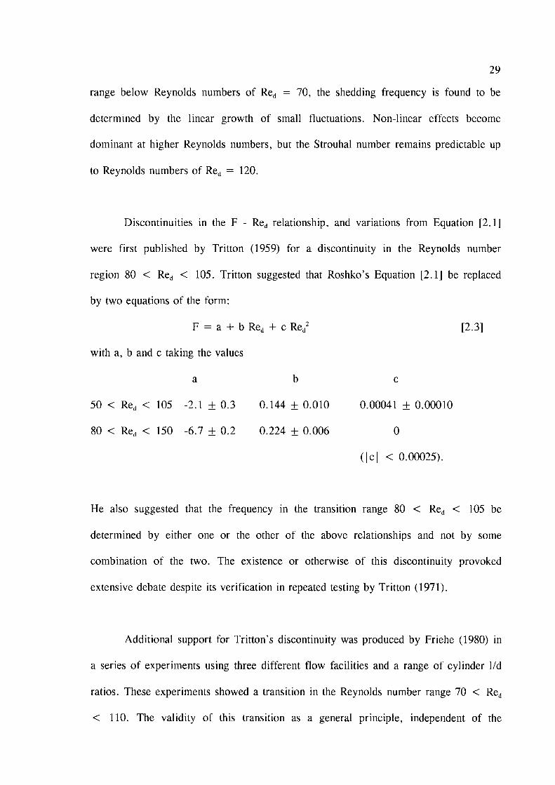
29

range below Reynolds numbers of Reo : 70, the shedding frequency is found to be

determined by the linear growth of small fluctuations. Non-linear effects become

dominant at higher Reynolds numbers, but the Strouhal number remains predictable up

to Reynolds numbers of Reo : 120.

Discontinuities in the F - Reo relationship, and variations from Equation [2.1]

were first published by Tritton (1959) for a discontinuity in the Reynolds number

region 80 < Reo ( 105. Tritton suggested that Roshko's Equation f2.ll be replaced

by two equations of the form:

F : a * b R e o * c R e o z

with a, b and c taking the values

a

< 105 -2. t + 0 .3 0.144

< 150 -6.7 + 0.2 0.224

+ 0.010 0.00041 + 0.00010

+ 0.006 0

12.31

50 ( Reo

80 < Reo

( lc l < 0 .00025) .

H e a l s o s u g g e s t e d t h a t t h e f r e q u e n c y i n t h e t r a n s i t i o n r a n g e 8 0 <

determined by either one or the other of the above relationships and not by some

combination of the two. The existence or otherwise of this discontinuity provoked

extensive debate despite its verification in repeated testing by Tritton (1971).

Additional support for Tritton's discontinuity was produced by Friehe (1980) in

a series of experiments using three different flow facilities and a range of cylinder l/d

ratios. These experiments showed a transition in the Reynolds number range 70 < Reo

30

ofpeculiarities of particular experimental arrangements, is discussed at the conclusion

this section in conjunction with the conclusions drawn from the following paragraphs.

The transition to turbulence in the wake of a circular cylinder was examined by

Bloor (1964) for Reynolds numbers from Reo : 200 to 50,000 , where the region

200 < Reo ( 400 was identified as Roshko's (1954) 'transition region' below which

no turbulent motion is generated. Bloor found that, within the transition region, the

position of the transition to turbulence moves towards the cylinder as the Reynolds

number is increased, and that the corresponding mode of transition is dominated by

large scale three-dimensionalities in the flow.

At Reo : 400, the vortices are turbulent on formation, and the location of the

transition is stable as Reynolds number is increased to 1,300 ; at higher Reo the region

of laminar flow begins to decrease, the region of transition almost reaching the

shoulder of the cylinder at Reo : 50,000. The mode of transition above Reu : 400 is

dominated by two-dimensional instability; this leads to the production of Tollmien-

Schlichting waves and eventually turbulence through small-scale three-dimensionalities.

The three-dimensional nature of the wake was investigated for stable,

transitional and turbulent vortices by Gerrard (1966a) using an array of hot-wire probes

along the cylinder length at Reynolds numbers of 85, 235 and 20,000. For the stable

vortex street Gerrard demonstrated that the shed vortices occur in straight lines inclined

to the cylinder axis, and suggested that modulations detected in the vortex shedding

frequency result from the wake flapping somewhat like a flag in the wind. In the

transitional region, Gerrard found the dominant three-dimensional feature to be the

3 1

simultaneous occurrence of laminar and turbulent vortices at different positions along

the cylinder length. He suggested that the vortex lines were now both wavy and

inclined. The turbulent vortices were found to form in straight lines parallel to the

cvlinder axis. with small random variations in inclination occurrine with time.

Gerrard (1966b) further examined the formation region of vortices for Reynolds

numbers greater than Reo : 400, and proposed the simultaneous existence of two

characteristic lengths, the length of the formation region, and the width of diffusion of

the shear layers. Because the length of the formation region decreases and the diffusion

width increases as the Reynolds number is increased, the resulting Strouhal number

remains approximately constant at St : 0.21 for Reynolds numbers Reo > 400. At the

time, Gerrard was not able to make reliable quantitative measurements of the vortex

shedding frequency to support his proposed underlying processes. Later Gerrard (1978)

conducted a comprehensive flow visualisation study of the wakes of cylinders in water

flow for Reynolds numbers from Reo : 0 to 2,000, using dye washed from the rear

surface of cylinders in a towing tank.

Gerrard's visual study outlined a series of flow regimes within the Reynolds

number range studied. The regimes were not separated by abrupt transitions, but were

observed to merge gradually into one another; and at the transition Reynolds number

the flow was found to change with time between regimes. These flow regimes are

summarised by Gerrard as follows:

0 < Reo < 34 Steady flow; standing eddies.

32

34 < Reo < l0 Wavy wake, no accumulation of dye into vortices.

55 < Reo < 100 Vortex street wake; remnants of the standing eddies still present;

diffusion of vorticity important.

100 < Reo ( 140 Increased efficiency of convective mass transfer behind the body;

an accelerating phase of vortex motion present up to Reo : 500.

140 < Reo < 500 Fingers of dye moving back towards the body from the wake;

vortex strength irregular; more nearly two-dimensional flow; transition to turbulent

vortex cores downstream.

250 < Reu ( 400 Transition to high Reo type of vortex shedding.

3s0

turbulence in the vortex cores on formation.

Gerrard qualifies these results with an observation on the sensitivity of the flow

to disturbances, in particular to the end conditions of the cylinder. He suggests that any

conclusions drawn from such experiments must be related to the experimental

arrangement involved. This is now recognised as one of the features of real turbulent

wakes shed from finite aspect ratio cylinders and also from large aspect ratio cylinders.

The three-dimensional effects caused by variations in flow velocity along

cylinder length were examined by Gaster (1969 and l97l) who suggested that

the

the

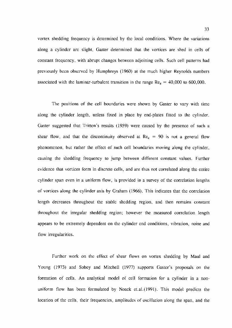
33

vortex shedding frequency is determined by the local conditions. Where the variations

along a cylinder are slight, Gaster determined that the vortices are shed in cells of

constant frequency, with abrupt changes between adjoining cells. Such cell patterns had

previously been observed by Humphreys (1960) at the much higher Reynolds numbers

associated with the laminar-turbulent transition in the range Reo : 40,000 to 600,000.

The positions of the cell boundaries were shown by Gaster to vary with time

along the cylinder length, unless fixed in place by end-plates fitted to the cylinder.

Gaster suggested that Tritton's results (1959) were caused by the presence of such a

shear flow, and that the discontinuity observed at Reo : 90 is not a general flow

phenomenon, but rather the effect of such cell boundaries moving along the cylinder,

causing the shedding frequency to jump between different constant values. Further

evidence that vortices form in discrete cells, and are thus not correlated along the entire

cylinder span even in a uniform flow, is provided in a survey of the correlation lengths

of vortices along the cylinder axis by Graham (1966). This indicates that the correlation

length decreases throughout the stable shedding region, and then remains constant

throughout the irregular shedding region; however the measured correlation length

appears to be extremely dependent on the cylinder end conditions, vibration, noise and

flow irregularities.

Further work on the effect of shear flows on vortex shedding by Maul and

Young (1973) and Sobey and Mitchell (1977) supports Gaster's proposals on the

formation of cells. An analytical model of cell formation for a cylinder in a non-

uniform flow has been formulated by Noack et.al.(1991). This model predicts the

location of the cells, their frequencies, amplitudes of oscillation along the span, and the

34

local shedding angle. It is shown to agree in general qualitative features with

experimentally observed cell properties.

The effect of end-plates on a vortex wake was investigated by Stansby (1974) by

measuring the variation of cylinder base pressure along the span. Stansby demonstrated

that end-plates could be used to produce a two-dimensional flow from an initial flow

with considerable spanwise variation. A more detailed examination by Graham (1969)

demonstrated that for aspect ratios (of the cylinder between the plates) less than four,

the flow becomes two-dimensional, and that at larger aspect ratios there is little or no

spanwise correlation between the vortex streets at positions a large distance apart,

suggesting that there are limitations on the spanwise influence of end-plates. These

limitations have been examined by Szepessy and Bearman (1992) for aspect ratios in

the range ( l/d : 0.25 - 12 ), and ( Reo : 8,000 - 140,000 ), by measurements of

spanwise correlation. The effect of changing aspect ratio is found to be Reynolds-

number dependent, having a weak effect at low Reo and a much stronger effect at

higher Reo. Thus two-dimensional flow is only produced by end-plates for small

cylinder aspect ratios at high Reynolds number.

A review of vortex shedding phenomena by Berger and Wille (1912) raised the

suggestion that variations in end conditions between different experimental

arrangements may be the basis of conflicting results, and that such variations may

become apparent in the observed inclination to the cylinder of the lines of shed

vortices. Strouhal numbers for 40 ( Reo ( 160 were also found to vary for different

levels of free stream turbulence between different facilities. A later review of vortex

shedding, by Bearman and Graham (1980), added further support to the influence of

3s

free stream turbulence on vortex shedding behaviour. These variations raise a problem

in relation to the use of Roshko's Equations [2.1] and [2.2] as a means of measuring

flow speed. However, investigations by Kohan and Schwarz (1913) suggest that once a

vortex-generating cylinder is calibrated for a particular facility, it remains an extremely

accurate tool for determining flow speed.

Variations in end conditions were examined by Slaouti and Gerrard (1981) by

visualisation of water flow over a vertical cylinder in a towing tank for Reynolds

numbers in the range Reo : 60 to 200. The effect of end conditions resulting from a

contaminated or clean water surface, from end plates and free ends, and from a gap

between the surface and a cylinder free end were examined.

All of these end conditions were found to dominate the flow near the cvlinder

ends, and thereby to influence strongly the complete wake structure. A further study of

the influence of end plates and free ends on vortex shedding behaviour, conducted by

Gerich and Eckelmann (1982), showed that frequency variations in the order of 10 -

15% could be produced up to 15 diameters from the cylinder ends by varying end

conditions.

The large influence of end conditions is supported by an examination of von

Karman's theory by Sirovich (1985), and experimental investigations by Sreenivasan

(1985), which indicate that the Strouhal-number / Reynolds-number relationship may be

partially indeterminate, with the outcome for particular regions of Reo being dependent

on the initial or boundary conditions.

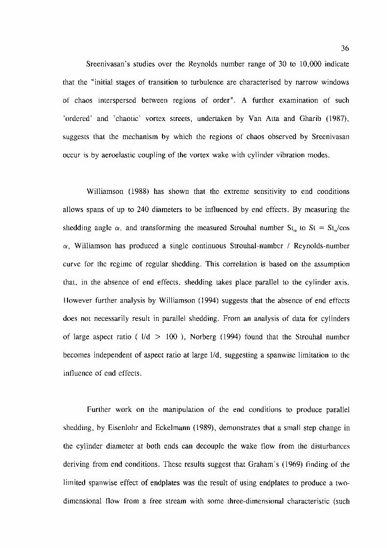
36

Sreenivasan's studies over the Reynolds number range of 30 to 10,000 indicate

that the "initial stages of transition to turbulence are characterised by narrow windows

of chaos interspersed between regions of order". A further examination of such

'ordered' and 'chaotic' vortex streets, undertaken by Van Atta and Gharib (1987),

suggests that the mechanism by which the regions of chaos observed by Sreenivasan

occur is by aeroelastic coupling of the vortex wake with cylinder vibration modes.

Williamson (1988) has shown that the extreme sensitivity to end conditions

allows spans of up to 240 diameters to be influenced by end effects. By measuring the

shedding angle a, and transforming the measured Strouhal number St. to St : St./cos

a, Williamson has produced a single continuous Strouhal-number / Reynolds-number

curye for the regime of regular shedding. This correlation is based on the assumption

that, in the absence of end effects, shedding takes place parallel to the cylinder axis.

However further analysis by Williamson (1994) suggests that the absence of end effects

does not necessarily result in parallel shedding. From an analysis of data for cylinders

of large aspect ratio ( l/d > 100 ), Norberg (1994) found that the Strouhal number

becomes independent of aspect ratio at large l/d, suggesting a spanwise limitation to the

influence of end effects.

Further work on the manipulation of the end conditions to produce parallel

shedding, by Eisenlohr and Eckelmann (1989), demonstrates that a small step change in

the cylinder diameter at both ends can decouple the wake flow from the disturbances

deriving from end conditions. These results suggest that Graham's (1969) finding of the

limited spanwise effect of endplates was the result of using endplates to produce a two-

dimensional flow from a free stream with some three-dimensional characteristic (such

37

as a transverse velocity gradient) rather than an independent effect of the end

conditions. A Strouhal-number/Reynolds-number relationship for parallel shedding has

been proposed by Fey et.al.(1998), based on their experimental data for parallel

shedding achieved by the use of either a step change in cylinder diameter or end plates

to control the end effects. Investigations by Konig et.al.(1990) indicate that the

Strouhal-number/Reynolds-number relationship is also influenced by the level of free

stream turbulence, particularly the exact location of the discontinuities in the

relationship.

An alternative method of decoupling the wake flow from the cylinder end

effects is proposed by Hammache and Gharib (1989) in which two control cylinders of

larger diameter, placed upstream of the test cylinder and normal to both the flow and

the test cylinder, are used to impose a symmetric pressure boundary condition at the

two ends of the cylinder. Further analysis by Hammache and Gharib (1991) of the

effects of non-symmetric pressure distribution along the span, indicates that the

resulting oblique shedding is a function of the induced spanwise flow in the base region

of the cylinder, and that a simple flow model based on the ratio of the streamwise to

the spanwise vorticity components allows the shedding angle to be predicted within two

degrees.

An analytical model based on a Ginzburg-Landau equation formulated by

Albarede and Monkewitz (1992) and Albarede and Provansal (1995) indicates that

symmetric end pressures may not produce parallel shedding but rather a symmetric

"chevron" pattern formed by oblique shedding growing inwards from both ends, and

that the oblique shedding observed for non-symmetric end pressures is a result of the

38

inward growing "half-chevron" with the larger shedding angle spreading across the

entire cylinder span.

Investigations by Anderson and Szewczyk (1997) and Ozono (1999) of the

effects of splitter plates in the near wake have shown that nominally two-dimensional

flows exhibit significant three-dimensional behaviour, which may be modified to appear

two-dimensional by manipulation of the cylinder radius (taper) or local free stream

velocity (shear layer flow), and by the use of splitter plates. The results of

manipulation of the shedding angle by the use of inclined end plates, obtained by

Prasad and Williamson (1997), indicate that the discontinuity in the Strouhal-number

variation in the vicinity of Reo : 250 does represent the infinite aspect ratio case, and

is not due to end conditions modifying the infinite aspect ratio behaviour. These results

suggest that, although particular experimental arrangements may be used to produce

vortex wakes which appear two-dimensional, the wakes are in fact always three

dimensional.

A review of developments in understanding cylinder wakes undertaken by

Williamson (1996) has emphasised the importance of the three-dimensional aspects of

nominally two-dimensional flows. Williamson also stresses the need to distinguish

between the "intrinsic" three-dimensional aspects of the flow arising from natural

instabilities, and the "extrinsic" three-dimensional aspects resulting from end conditions

and other external effects.

The investigations of vortex shedding from circular cylinders normal to the flow

provide a base of knowledge in flow mechanisms and experimental techniques which is

39

applicable to the more complex problem of vortex shedding from yawed cylinders. In

particular these investigations have revealed major sources of uncontrolled experimental

variation such as cylinder end effects, free stream shear flows and turbulence levels,

and aeroelastic and other vibrations.

For cylinders normal to the flow, the effects of cylinder end conditions and

free-stream shear flows may be considered to have been negated in experimental

arrangements where either symmetric or parallel vortex shedding is observed. This

principle may not be extended to the case of yawed cylinders where the presence of

both normal and axial components of vorticity results in a net vorticity vector which

may produce lines of shed vortices which are inclined to the cylinder axis. However,

the success of Hammache and Gharib (1991) in determining shedding angles for

cylinders normal to a shear flow by the calculation of spanwise and streamwise

vorticity components suggests that a similar method may be applicable to yawed

cylinders in a uniform flow. A numerical simulation of the vortex wake by Jordan and

Ragab (1998), using the large eddy simulation method, has reliably reproduced

previous experimental results for the velocity in the near wake. This raises the

possibility of reliable numerical simulation of the yawed cylinder wake in the future.

40

2.5 Vortex Shedding from Cylinders at Angles of Yaw.

Previous investigations of vortex shedding from yawed circular cylinders have

concentrated on the effect of deviations in cylinder alignment from the normal flow

case. Such studies do not extend to small angles of yaw from the axial direction

( i . e . s m a l l 6 ) . T h e i r p r i m a r y c o n c e r n i s w i t h t h e r a n g e 9 0 " >

emphasis on describing the vortex shedding process as a variation from the normal

cylinder case. Initial experiments on vortex shedding from cylinders at small yaw

angles were conducted in the Department of Mechanical Engineering in the University

of Adelaide by final-year undergraduate students Azadegan (1987) and Circelli (1988).

In both cases the results indicated the presence of vortex shedding when 0 is small.

Hot-wire studies by Hanson (1966), of vortex shedding from cylinders at yaw

angles from p : 90o to 18', formed the basis for the application of the so-called

'independence principle' to vortex shedding from yawed cylinders. The 'independence

principle' asserts that the shedding frequency is determined solely by the component of

flow velocity normal to the cylinder axis, and is independent of the axial velocity

component. Hanson's investigations are within Roshko's (1954) 'stable' range of

Reynolds number (from Reo : 40 to 150), in which the vortex shedding behaviour of a

normal cylinder is described by Roshko's Equation 12.ll. Hanson uses the

independence principle to reformulate Equation [2.1] for yawed cylinders in the stable

shedding range as:

F : 0.212 Re, - 4.5

where Ren : Reo sin B.

12.41

4 l

Hanson's results for angles p of 90, 63,45,34,22 and 18 degrees show good

agreement with Equation 12.41 except for the data at p : 18'. In addition, Hanson

found the critical Reynolds number (at which vortex shedding first occurs), based on

the normal component of the flow, to be approximately constant for 6 > 40'. From

these observations Hanson concludes that Equation 12.4] is a useful measure of the

effect of cylinder yaw on the frequency of vortex shedding. Support for this conclusion

comes from the experiments of Surrey and Surrey (1967) who examined cylinders at

similarly large yaw angles, but at much higher Reynolds numbers (4,000 - 65,000).

With decreasing yaw angle, their Strouhal number based on the normal velocity

component remains approximately constant, and correspondingly the energy of the shed

vortices decreases in significance, becoming negligible in comparison with the general

wake turbulence at 6 < 50'.

An analytical study of fluid flow over yawed cylinders was undertaken by Chiu

and Lienhard (1967). Based on their theoretical investigation of boundary-layer

formation and separation, they found the vortex-shedding behaviour to be determined

solely by the cross-flow in the region of large 0 and high Reo. These conclusions were

supported by experiments conducted by Chiu (1966) in the Reynolds number range

3 , 9 0 0 ( R e o < 2 | , 2 0 0 f o r a n g l e s o f y a w i n t h e r a n g e 3 0 . <

Lienhard's investigation of the region of validity of Equation 12.41 suggests that large

deviations from the independence principle can be expected for Reo < 300 where the

wake thickness begins to vary with Reynolds number. Van Atta (1968), who initially

intended to examine the anomaly in Hanson's (1966) results for p : 18o, showed that

many of Hanson's data were affected by locking of the vortex-shedding frequency to

the cylinder's natural vibrational frequency.

42

A further investigation of such aeroelastic coupling, between structural

vibrations and fluid forces, was conducted by King (1977) for yawed cylinders in the

range 45' < p < 90'. King observed such coupling for the wide range of Reynolds

numbers from Reo : 2,000 to 20,000.

Van Atta (1968) examined the "lock-in" process by using a phonograph

cartridge to detect cylinder vibrations, while varying the natural frequency by adjusting

the cylinder tension. These investigations demonstrated that lock-in tends to occur by a

lowering of the shedding frequency to that of a natural vibration mode near the

frequency given by Equation p.al. Van Atta suggests that this behaviour indicates that

the cross-flow alone excites cylinder vibrations, and that this effect explains why

Hanson's frequency observations can be reduced to Equation 12.41.

Van Atta (1968) proceeded to investigate vortex shedding from non-vibrating

cylinders over the Reynolds number range 50 < Reo ( 600 at angles of yaw from

0 : 90' to 14". For these flow conditions, Van Atta obtained results at constant

normal Reynolds numbers of Ren : 50, 80 and 150 which indicate that the

independence principle is invalid for angles of yaw P < 60'. This suggests that the

components of flow are not independent, but that at large angles of yaw (large p) the

vortex shedding behaviour is very heavily dominated by the normal flow component.

Experiments were made at higher Reynolds numbers by Smith et al. (1972). While

their measured vortex-shedding frequencies are consistent the independence principle in

the range 1,000 ( Reo ( 10,000 for p : 90o to 30', their detailed examination of

wake properties shows that the cylinder base pressure and the position of the transition

to turbulence do not obey the independence principle.

43

T h e R e y n o l d s n u m b e r r a n g e b e t w e e n v a n A t t a , s ( 1 9 6 8 ) r e s u l t s ( R e o <

and Smith's (1972) results (Reo ) 1000) was examined by Knaus et al. (1976) for a

yaw angle of p : 50". Their results show that for 390 < Reo ( 1560 the vortex

shedding frequency is 8 - l0% higher than that predicted by the independence

principle, with a trend toward the predicted values at increasing Rea.

A detailed study by Ramberg (1983), of both stationary and vibrating yawed

cylinders in the Reynolds number range Reo : 150 to 1,100 , for angles of yaw

0 : 90'to 30', examined the effect of end conditions on the vortex shedding process.

Ramberg examined the vortex shedding angle a by using a strobe light to illuminate

aerosol particles in an air flow. These observations indicate that the cylinder end

conditions can dominate the wake behaviour for spans of up to 100 diameters. Ramberg

observed that in the absence of end effects shedding occurs with the vortex lines

inclined to the cylinder axis; he supports this observation with physical arguments that

such inclined shedding results from the presence of a component of vorticity associated

with the axial flow component, which causes the net vorticity vector to be inclined to

the cylinder axis. Ramberg's observations of vibrating yawed cylinders indicate that

shedding parallel to the cylinder axis occurs when the vortex shedding frequency locks-

in to the cylinder vibrational frequency.

Ramberg's observations and arguments for inclined vortex shedding suggest that

the independence principle has no validity, except in specific cases, such as that of

vibrating cylinders. His observation that the shedding frequency may vary with changes

in the shedding angle, caused by non-ideal end conditions, suggests that previous

results may have also been subject to such variation.

44

In the investigation by Shirakashi et al.(1986) for Reo : 800 to 55,000 and

angles of yaw from p : 45" to 90', flow visualisation by smoke streaks showed that

the flow over a yawed cylinder is highly three-dimensional in nature. Only when the

secondary flow behind the cylinder is suppressed (by plates in the cylinder wake) does

the shedding frequency become equal to that for a cylinder subject to only the normal

velocity component of the flow. From these observations, it was concluded that data

correlations resulting from the application of the independence principle are largely

fortuitous.

Computational analysis by Kawamura and Hayashi (1994) of the wake of a

yawed cylinder at p :60o, Reo : 2,000 for cylinders of both finite and infinite aspect

ratio ( l/d < 15 and l/d : oo ) indicate a weak three-dimensional spanwise structure

for the infinite cylinder accompanied by a secondary flow propagating downstream

along the cylinder axis, and a strong three-dimensional structure for the finite aspect

ratio cylinders. An experimental analysis of the wake by Hayashi and Kawamura

(1995) ( for 0 : 60o, 45o and 30'; Reo : 15,000; l ld:20 ) identif ied a quasi-two-

dimensional region of the wake ( such that the flow has a similar pattern in any section

parallel to the free stream ) along the receding half of the span.

These results raise the possibility that for cylinders of large aspect ratio

(l/d > 100), a quasi-two-dimensional flow may be established over the majority of the

span where the secondary flow propagating along the cylinder axis has become fully

developed. As B is decreased this secondary flow is expected to increase in strength

and thus require a greater length to develop, or, alternatively, to continue to develop

without ever establishing the fully developed state required for quasi-two-dimensional

flow.

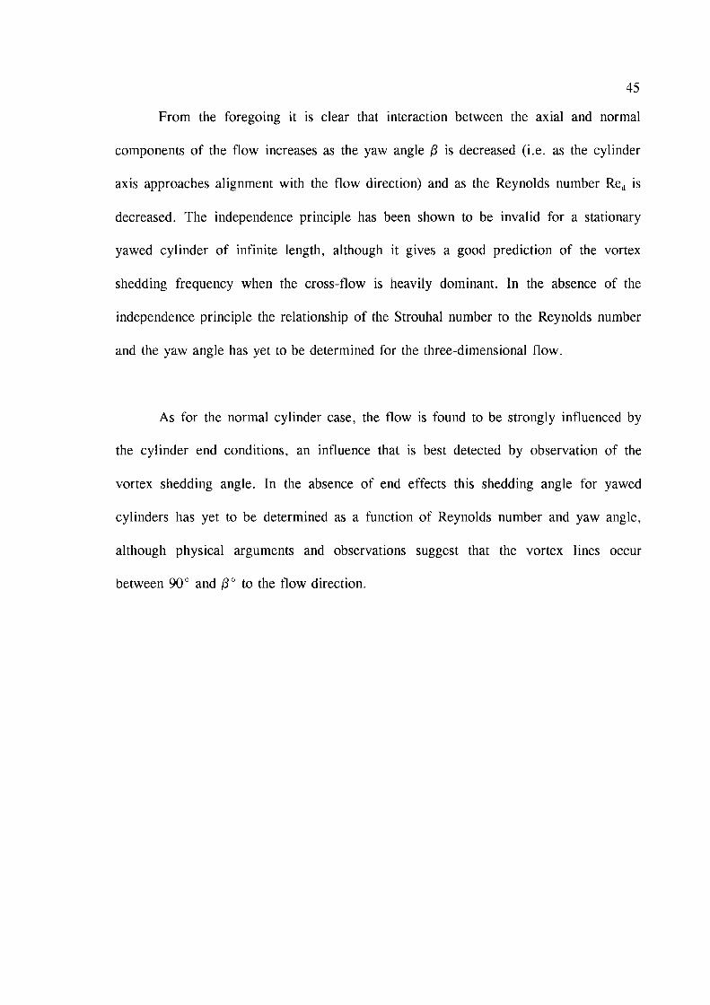
45

From the foregoing it is clear that interaction between the axial and normal

components of the flow increases as the yaw angle p is decreased (i.e. as the cylinder

axis approaches alignment with the flow direction) and as the Reynolds number Reo is

decreased. The independence principle has been shown to be invalid for a stationary

yawed cylinder of infinite length, although it gives a good prediction of the vortex

shedding frequency when the cross-flow is heavily dominant. In the absence of the

independence principle the relationship of the Strouhal number to the Reynolds number

and the yaw angle has yet to be determined for the three-dimensional flow.

As for the normal cylinder case, the flow is found to be strongly influenced by

the cylinder end conditions, an influence that is best detected by observation of the

vortex shedding angle. In the absence of end effects this shedding angle for yawed

cylinders has yet to be determined as a function of Reynolds number and yaw angle,

although physical arguments and observations suggest that the vortex lines occur

between 90' and 6o to the flow direction.

46

2.6 Literature Review: Kev Conclusions.

1. The overall mechanism for the production of turbulence in the planar

boundary layer is not yet fully understood; however, the dominant mechanisms may be

described by the burst cycle.

2 . F o r c y l i n d e r s o f s m a l l t r a n s V e r s e c u r v a t u r e ( 6 / a <

mechanisms within the axisymmetric boundary layer appear to be similar to those of

the planar boundary layer.

3. For cylinders of moderate transverse curvature ( 5 < 6la < 20 ), a burst

cycle similar to the planar mechanism appears with the addition of large turbulent

cross-flows.

4 . F o r c y l i n d e r s o f l a r g e t r a n S V e r S e c u r v a t u r e ( 6 l a >

axisymmetric boundary layer takes on a wake-like character, and the relative

importance of the burst cycle and of the turbulent cross flows in the production of

turbulence is not yet fully understood.

5. The ratio of the volume of a boundary layer to the surface area supporting it

is greater for a slender cylinder in axial flow than for a flat plate by a factor of the

order of 612a, which may be as high as 20 or more. This observation suggests the

presence of a more efficient vorticity-generation mechanism, possibly related to

turbulent cross-flows, than occurs in planar boundary layers.

47

6. The axial boundary layer on a slender cylinder is maintained for small

angles of inclination 0 between the cylinder axis and the flow direction. The shape of

the boundary layer cross-section becomes increasingly elongated to the leeward side of

the cylinder with increasing p. and shows marked asymmetry at angles of yaw as small

a s 6 : 1 . 0 o .

1. The vortices shed from a cylinder normal to the flow may be generated with

their axes either parallel to the cylinder axis or in the form of symmetric chevrons, in

the absence of end effects and three-dimensional flow characteristics in the free stream.

8. For cylinders normal to the flow, the vortex-shedding frequency at constant

Reynolds number will vary with changes in end-conditions, since the end-conditions

affect the angle between the vortex lines and the cylinder axis. Such variations appear

to be the cause of discontinuities in the Reynolds-number / Strouhal-number

relationship which are not always reproducible under different experimental

arrangements.

9. The independence principle, (the notion that velocity components normal and

parallel to the cylinder axis produce independent effects) has been shown to give a

good prediction of the vortex-shedding frequency of a yawed cylinder for large angles

of yaw (i.e. close to normal flow) - but only in this case.

10. For cylinders with their axes inclined to the flow, the interaction between

the axial and normal components of the flow becomes very significant as the cylinder

yaw angle is decreased (approaching axial flow), and as the Reynolds number is

decreased.

48

1 1. The independence principle has been shown to be invalid for a long slender

(stationary) cylinder with its axis yawed to the flow direction, but the functional

dependence of vortex-shedding frequency on flow parameters at small yaw angles has

not previously been determined.

12. For cylinders with their axes inclined to the flow, the vortex lines are

inclined to the flow at an angle greater than the cylinder yaw angle. In previous work,

the relationship between the vortex angle and the yaw angle, as a function of the flow

parameters, has not been established.

49

3. FACILITIES AND PROCEDURES

3.1 Low Speed Wind Tunnel

Experiments were conducted in the variable width, 3 metre long test section of

the closed-circuit low speed wind tunnel shown in Figure t3.1l.The air speed in the

test section can be continuously varied from 0 to 2J mls, although the minimum stable

speed is approximately 1 m/s. The airflow is generated by a belt-driven axial fan

located between the first and second corners, powered by a variable speed electric

motor mounted outside the tunnel on rubber vibration isolators.

The quality of the air flow entering the test section is maintained by a settling

chamber containing a series of wire screens, followed by an octagonal to rectangular

contraction with an area ratio of 4:1 upstream of the test section. The return circuit

consists of a long diffuser with turning vanes at each corner. The entry to the return

circuit consists of a bell-mouth inlet fitted with a wire screen to prevent the entry of

foreign objects.

The air temperature within the wind tunnel is maintained constant by means of

air exchange with the laboratory air, which is cooled by a large air-conditioning

system, and may be regulated to within 1 degree. The air exchange is achieved by an

adjustable vent in the low velocity section of the tunnel, upstream of the contraction,

allowing high pressure heated air from the tunnel to be expelled, while additional cool

air is introduced via the bell-mouth inlet upstream of the fan.

s0

Air ExchanseOutlet

-

Screens__)

Octagonal Section

Test Section

I-.----.-E650 mm

Test Section

s^t"w IScreen

300 mm

Corner Turninsvanes Bell Mouth

Inlet

Figure 3.1 Closed-Circuit Low-Speed wind tunnel

Department of Mechanical Engineering

The University of Adelaide.

5 1

3.1.1 Variable-width test section

As the proposed experimental investigations made use of the full length of the

wind tunnel test section, it was necessary to design and build a new test section capable

of providing a uniform velocity distribution in the streamwise direction. This variable

width test section consists of a wooden base supporting a perspex top at a height of 300

mm, and adjustable perspex side walls as shown in Figure[3.2]. The initial width at the

upstream end is fixed at 650 mm to match the contraction outlet. A series of four screw

jacks equally spaced along the test section length allow the section width to be varied

along the section length, to a maximum of + 200 mm at the downstream end. This

allows for the establishment of a pressure gradient along the section length, or

alternatively, allows for a correction to be made to remove any unwanted pressure

gradient associated with boundary-layer growth on either the tunnel walls or the test

cylinder, and thus to provide a uniform streamwise velocity distribution.

AdiustableSide Walls

AdjustuentScrew Jack

Figure 3.2 Variable-width Test Section.

52

3.1.2 Free-stream velocitv

The mean velocity in the free stream was measured by means of a pitot-static

tube, located at the same downstream location in the test section as the experiments in

progress. The dynamic pressure of the air flow was measured by a null-balance

manometer with a resolution of 0.01 mm and a maximum reading of 30 mm, using a

manometer fluid of specific gravity 0.826. A water manometer with a resolution of 0.2

mm was used at higher velocities ( above 22 mls ) where the dynamic pressure

exceeded the range of the more accurate null-balance manometer.

The mean free stream velocity of the air U, was calculated from the measured

dynamic pressure and the ambient air density as:

lJ, : {(2ghp^lp^) , [3. 1]

where h : ffiea,sured manometer head (m)

g : acceleration due to gravity (m/s2)

pm : manometer fluid density (kg/m3)

p, : ambient air density 1kg/m3) .

The ambient air density was calculated from the perfect gas equation of state

using the measured air temperature and pressure as:

( _ I [3 .2]I P, le o = l n r l[ , J

where Pu : ambient air pressure (Pa)

Tu : ambient air temperature (K)

R : Specific Gas Constant (287 J/kg.K for air ) .

Reynolds numbers were calculated

based on the ambient temperature T" and

and Chow 1976\:

using a value of

evaluated by the

53

absolute viscosity of air p,

Sutherland equation (Kuethe

Tr*120

rj6 t3.31

where the reference values of temperature and viscosity are those for standard sea level

conditions:

: 2 8 8 . 1 6 K

: 17.894 x 10{ kg/m.s

The turbulence intensitv of the free-stream air flow was found to be 0.ll% bv

hot wire anemometry using a single wire probe located on the test section centreline.

It]'ut a_ =u^

To

lto

54

3.I.3 Streamwise velocitv variation

Initial measurements were made of the streamwise velocity variation within the

rectangular test section with the side-walls parallel; two null-balance manometers were

used to measure the dynamic pressure at locations 500 mm and 2700 mm downstream

of the entry to the test section. These measurements indicated a 5 % rise in the mean

velocity over this distance for flow at the downstream section at20 mls, increasing to a

l0% rrse at 4 mls.

A traverse system was constructed to move a hot wire probe along the full

length (3 metres) of the test section centreline as shown in Figure t3.31. The probe is

supported above a metal slider which is guided along the centre of the test section floor

WireStays

Hot-WireProbe

Thumb Wheel

Draw String

Contraction Test Section 3000 mm

DownstreamSupport

Clamp

Figure 3.3 Streamwise HorWire Probe Traverse.

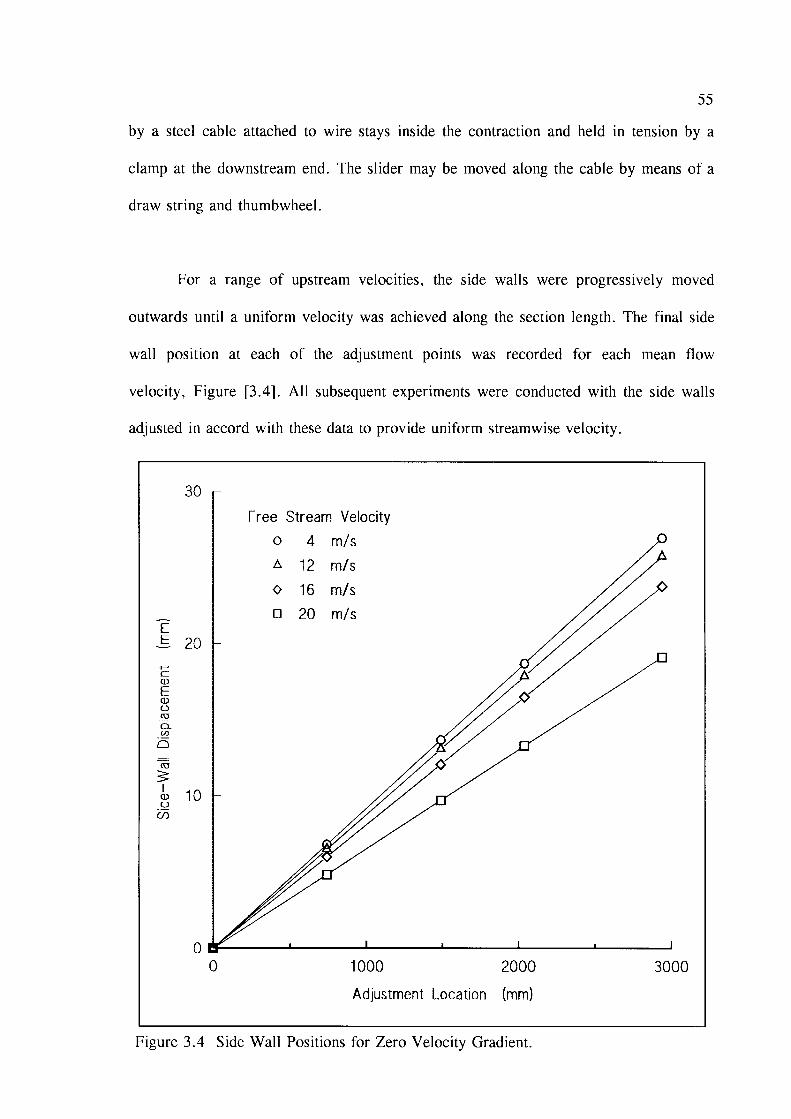
55

by a steel cable attached to wire stays inside the contraction and held in tension by a

clamp at the downstream end. The slider may be moved along the cable by means of a

draw string and thumbwheel.

For a range of upstream velocities, the side walls were progressively moved

outwards until a uniform velocity was achieved along the section length. The final side

wall position at each of the adjustment points was recorded for each mean flow

velocity, Figure 13.41. All subsequent experiments were conducted with the side walls

adjusted in accord with these data to provide uniform streamwise velocity.

Free Stream Velocity

o 4 m/sa 12 m/s

o 16 m/str 20 m/s

ct r . n-= lV

Cq)Cq)

-o-

- aO

(s

I

b 1 0E(n

1000

Adjustment Location

2000

(mm)

3000

Figure 3.4 Side Wall Positions for Zero Velocity Gradient.

3.I.4 Test-cylinder arrangement

The circular cylinders tested consisted of lengths of nylon line, of diameter 0.90

mm, 1.93 mm and2.95 mm. In each case the cylinder was anchored at the upstream

end by wire stays in the wind tunnel contraction, and held in tension at the downstream

end by means of a pulley and a weight, as shown in Figure t3.51. The cylinder yaw

angle may be varied from 0o to 12" by moving the pulley horizontally across the end

of the test section. and by adjusting the lengths of the upstream supports.

For axial flow, the test cylinder was initially aligned relative to the test section

walls. Final alignment was achieved by measuring the boundary layer velocity profile

on either side of (and above and below) the cylinder, and making incremental

adjustments to the upstream supports until boundary layer symmetry was achieved. In

all cases the initial geometrical alignment was found to have been within 0.1" of the

final alignment. For near axial flow cases the cylinder yaw angle was determined by

measuring the cylinder's horizontal displacement from the axial alignment position

using a micrometer surface gauge with a resolution of 0.01 mm.

The frequency of natural vibration of the test cylinders can be varied by altering

the tension by adding incremental weights to the initial 5kg weight. This enabled the

natural frequency to be separated from any fluid related forcing frequency. These

adjustments were performed whenever the measured periodic velocity variations in the

flow were observed to lock on to a single frequency (a vibration harmonic) rather than

to vary about a mean fluid frequency; such adjustments can be made without the need

to calculate the cylinders natural frequency and harmonics.

57

o0

';; b0- . H

H ( D

f B

oaX e

t r Eo €

o

g ' 6} FE . | i9 €E AU ) H

v)(tlo

>.(t)

t t u

---"'l{)O

= a )! v . -

. 9 4E e i5 XJ . v

tr)z

oa)(t)

v)oF

4

A. l!o

o !> . t rc q O

I t \(n \./( ) _

EF

d Eo U''hE- og u. o r t.IJ OOv ) =

f , . !<tr

Figure 3.5 Test Cylinder End Supports.

5 8

3.2 Flow Visualisation in Air

Visualisation of the air flow is achieved by means of smoke produced by the

vaporisation of a film of oil from an electrically heated wire. Two arrangements of

such 'smoke wires' were used in the wind tunnel test section. A single smoke wire

(shown in Figure [3.6]), positioned vertically through the test section, and passing

adjacent to the test cylinder, is coated with oil which forms into regularly spaced beads

along the wire. An electric current is used to heat the wire, causing the beads of oil to

vaporise and form regularly spaced streamlines of smoke. The oil coating is applied to

the wire by pulling the wire through an oil reservoir located on top of the test section.

The wire is held straight by small tensioning weights as shown in Figure [3.6]. The

smoke streaks were illuminated by spotlights and filmed on video.

o*^r_^ CylinderJlnOKE

TEST SECTIONEND VIEW.

Smoke Streaks

TEST SECTION SIDE VIEWS

Figure 3.6 Vertical Smoke Wire.

59

Two video systems were used, a conventional 25 frame/second VHS system,

and a high speed Kodak Ekta Pro video system capable of recording 1000

frames/second. The limited amount of light reflected by the smoke particles restricted

the use of the high speed system to less than 100 frames/second.

A second smoke wire arrangement, shown in Figure 13.71, is used to generate

smoke from the surface of the test cvlinder. A ceramic insert in a hollow 2.95 mm

diameter cylinder is wound with resistance wire which may be electrically heated by a

power connection through the centre of the downstream cylinder length. An oil coating

is applied manually with a small artist's-paint-brush. The lighting and video recording

arrangements are similar to those for the vertical smoke wire with the addition of a

mirror arranged to direct some of the camera's field of view to an oscilloscope screen

displaying the voltage output from a horwire anemometer.

- Miror

TEST SECTIONEND VIEW

Oscilloscope Anemometer

I( t-\ - - _ - +

. . . .-_l--l

. Ceramic Wire Wound Smoke Generator I I! , l l

- - t \

Figure 3.7 Surface Smoke Generation with Simultaneous Hot-Wire Anemometry.

60

3.3 Hot Wire Anemometry

A four channel TSI IFA-100 constant temperature hot wire anemometer with an

overheat ratio set to 1.8 was used for velocitv measurements in the air flow. The

voltage output may be either the total DC voltage or the fluctuating AC component. In

the DC mode a range of time constants are available (low pass filters) to produce time

averages of the mean voltage output. The frequency response of each anemometer

channel may be adjusted by varying the bridge and cable compensation while viewing

the output voltage response to an inbuilt square wave generator.

Identical signal conditioners are available for each anemometer, allowing the

output voltage to be offset, amplified and filtered while maintaining time correlation

between channels. The offset may be set in one volt increments between 0 and 9 volts.

The gain may be set between 1 and 900 as a single digit mantissa (1 - 9) and an

exponent of 0, 1 or 2. The filter is a third-order Sallen-Key type (-18dB/octave), with a

low pass setting range from 1 Hz to 400,000 Hz entered as a single digit mantissa and

an exponent of 0 through 9.

A horizontal traverse system was constructed to support two micrometer surface

gauges (reading + 0.01 mm), which were used to position the hot-wire probes in the

vertical direction as shown in Figure t3.81.

The location

optically by means

of

of

the probes relative to the cylinder surface was determined

a small telescope (with cross hairs), clamped to a vertical

6 1

column. The telescope height may be adjusted coarsely by varying the clamping

position, and very precisely over a 10 mm range by a vernier micrometer (also shown

in Figure t3.81). Vertical displacements may be measured to an accuracy of + 0.05

mm by aligning the telescope so that the cross hairs intersect on the active length of the

hot wire probe, setting the vernier scale to zero, and then adjusting the micrometer

until the cross hairs intersect on the cvlinder surface.

When two probes are used together, the vertical displacement between them

may be measured in a similar manner. The horizontal displacement between them may

be determined by initially optically aligning the probes in the vertical direction, and

then measuring subsequent displacements of the horizontal traverse using a pair of

vernier callipers.

Guide Rail Top of Test Section

t/'-- --j:-m1 slot

Traverse Base Plate /

SurfaceGauge

VerticalSupportColumn

Telescope

Ir t

' ' \

, , , O f

Vernier

,f

,l'Ajusmet

3 m m R o d - :..- J mm Rod Clamp

H.W. hobe / Sight Line -

Figure 3.8 Hot Wire Probe Positioning Traverse and optical alignment system.

3.3.1 Probe desisn

For velocity measurements in the free stream, or in the outer boundary layer,

the u-component (streamwise component) is measured using a 4pm-diameter tungsten

wire with an active length of 1 mm, giving a length to diameter ratio of 200, and a

typical cold resistance of 6.5 Ohms. Two probe designs were used, a straight probe

shown in Figure [3.9(a)], and a 90' angled probe shown in Figure t3.9(b)1. In both

these probe designs the ends of the tungsten wire are copper coated, and then soft

soldered to the ends of steel needles supported in a two core ceramic rod.

For u-component velocity measurements close to the cylinder surface, it is

necessary to minimise the active length of the probe in order to minimise the variation

in y (distance to the surface) along the active length of the probe due to the transverse

curvature of the cylinder surface. In the inner boundary layer, a straight probe with a

0.3 mm active length of 2.5 pm-diameter Wollaston wire (90% Pt, 10% Rd) is used,

giving a length to diameter ratio of 120. The probe construction is shown in Figure

[3.9(c)], and is similar to that of the straight tungsten wire probe except that the hot

wire projects forward of the ends of the supporting needles, allowing for greater

accuracy in optically determining the position of the active length.

For u and v-component (streamwise and radial) velocity measurements, a cross-

wire probe is used with two matched-resistance, 2.5 p"m-diameter Wollaston wires of

active length 0.3 mm. The hot wires are soft soldered to steel needles held in a four

core ceramic rod, with the protruding ends inclined at 45' to the rod as shown in

Figure t3.9(d)1.

63

2 Corc Cerarnic Rod J

Q 2 m m

(a) Straight (4pm Tungsten Wire)

I

Steel Needles J

Steel Needles

(b) Angled (4 pm Tungsten Wire)

2 Core Ceramic Rod

Steel Needlss i

(c) Straight (2.5 pm Wollaslel Wire)

2 Core Ceramic Rod

Figure 3.9 Hot Wire Probe Design.

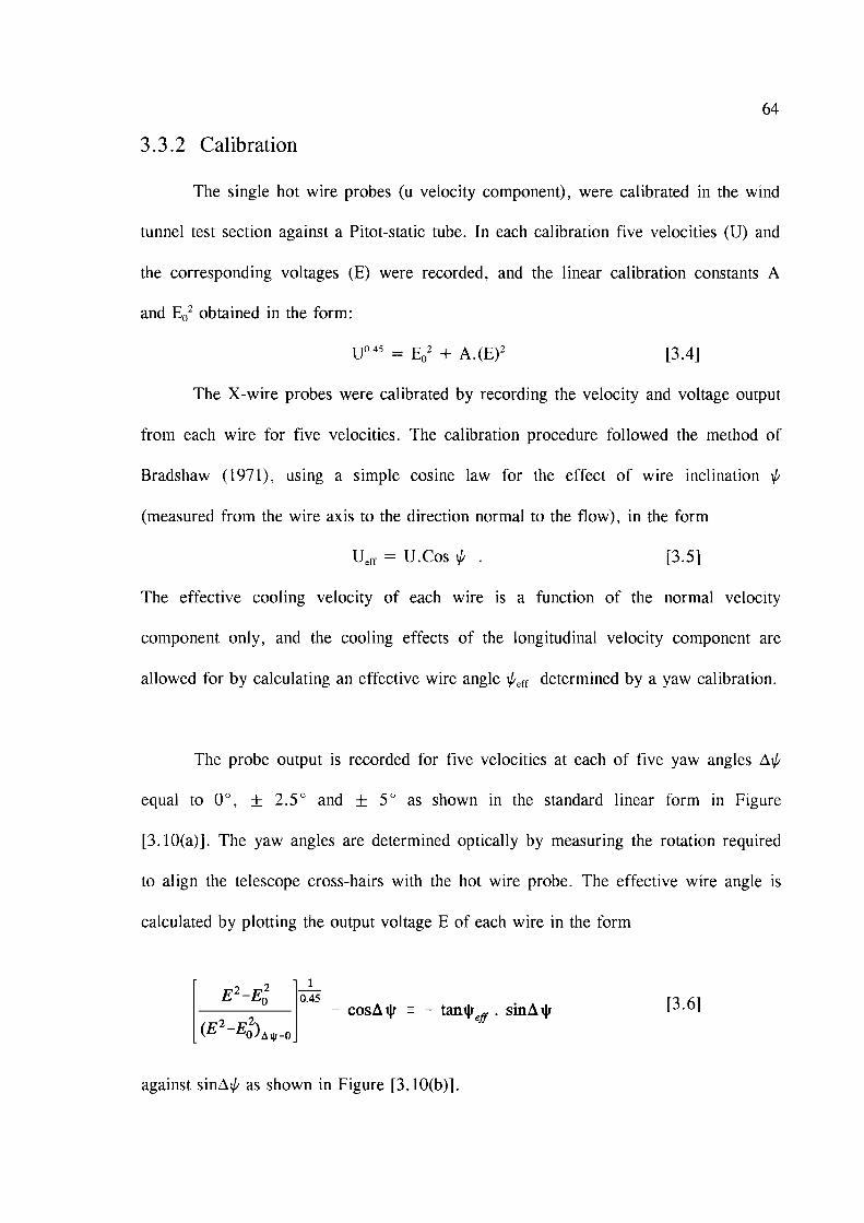
3.3.2 Calibration

The single hot wire probes (u velocity component), were calibrated in the wind

tunnel test section against a Pitot-static tube. In each calibration five velocities (U) and

the corresponding voltages (E) were recorded, and the linear calibration constants A

and En2 obtained in the form:

u o a 5 - E o t * A . ( E ) '

The X-wire probes were calibrated by recording the velocity and voltage output

from each wire for five velocities. The calibration procedure followed the method of

Bradshaw (1971), using a simple cosine law for the effect of wire inclination r/

(measured from the wire axis to the direction normal to the flow). in the form

U"n : U.Cos r/ t3.sl

The effective cooling velocity of each wire is a function of the normal velocity

component only, and the cooling effects of the longitudinal velocity component are

allowed for by calculating an effective wire angle ry'"6 determined by a yaw calibration.

The probe output is recorded for five velocities at each of five yaw angles Ary'

equal to 0", + 2.5" and + 5o as shown in the standard linear form in Figure

[3.10(a)]. The yaw angles are determined optically by measuring the rotation required

to align the telescope cross-hairs with the hot wire probe. The effective wire angle is

calculated by plotting the output voltage E of each wire in the form

E2-4I

0.45

13.41

(E'-Et) ov=o

- cosArf = - tanf"n. sinA$

against sinAr/ as shown in Figure t3.10(b)1.

t3.61

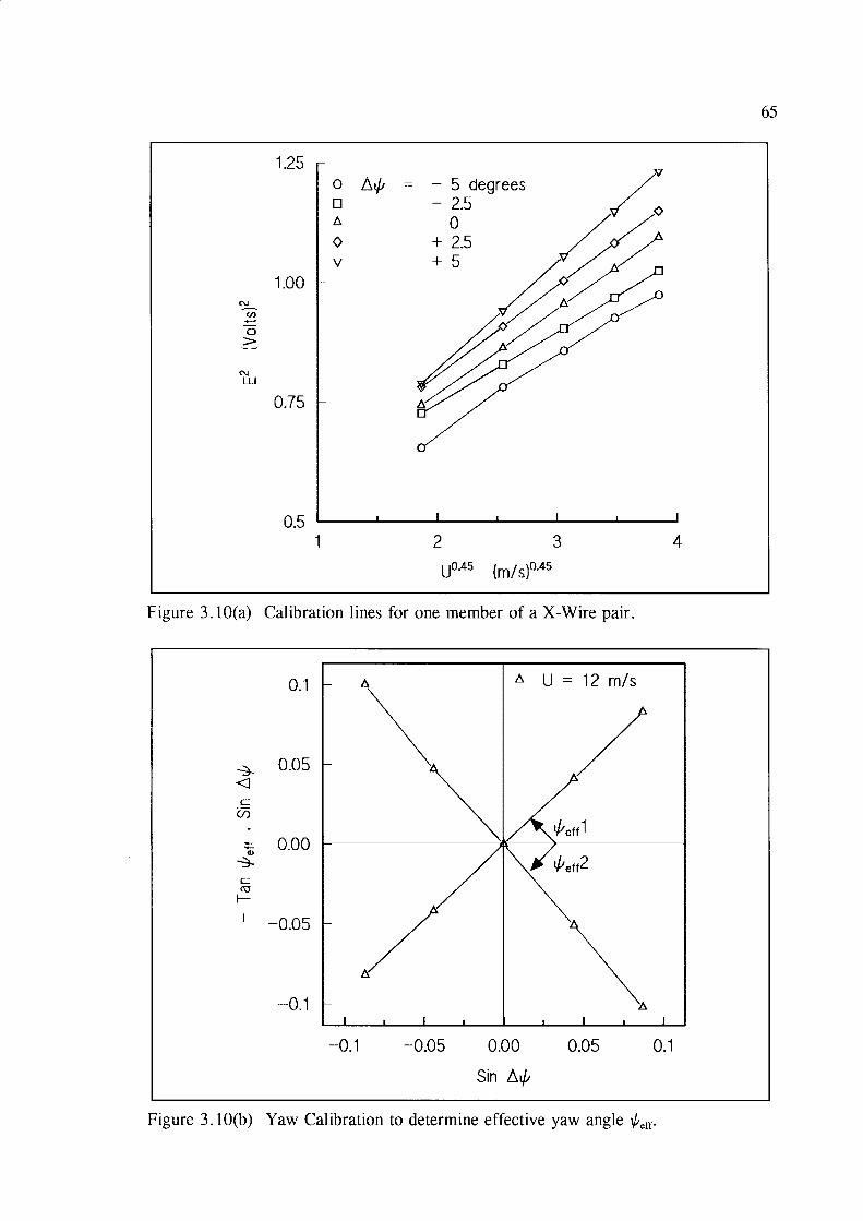
65

otrA

oV

1.25

1.00N

(t

o-

NLU

0.75

0.5

U0.4s (m/s)0.45

Figure 3.10(a) Calibration lines for one member of a X-Wire pair.

0.1 U = 1 2 m / s

*"ttl

. t

y' **?

->

. g

0-+c(U

F

I

0.05

0.00

-0.05

-0.1

-0.1 -0.05 0.00

Sin Arl

0.05 0.1

Figure 3.10(b) Yaw Calibration to determine effective yaw angle ry'.,r.

3.3.3 Digital data acquisition

After filtering the IFA-300 anemometer output voltage at 10 kHz, the analogue

data were digitised by either of two methods. In the first method the anemometer

output voltage is digitised by both a Hewlett-Packard-3582A Spectrum Analyser and a

Phillips PM 3310-60 MHz digital storage oscilloscope as shown in Figure [3.11(a)]. In

the second method the filtered anemometer output voltage is digitised by an RTI-860

analogue-to-digital converter at 20 kHz, and the digitised data recorded by an 80386

micro processor as shown in Figure t3.11(b)1. Up to four channels of anemometer

output voltage may be digitised simultaneously using this method, and the 80386

processor is then used to convert the voltage data to velocity data using the appropriate

calibration information, and to perform any subsequent data analysis.

U)(l)

Fr

B\

(a) Method 1.

oov

F\\o€

I

F&

(b) Method 2.

Ha

f r

, N

x

Figure 3.11 Digital Data Acquisit ion

61

3.4 Recirculating Water Tunnel

A recirculating water tunnel, shown in Figure [3.12], was designed and

constructed for hydrogen-bubble flow-visualisation. The working section of the tunnel

consisted of a 3.5 metre long open-topped perspex channel 475 mm deep and 175 mm

wide, filled with water to a depth of 450 mm. The flow quality was controlled by a

settling chamber 700 mm wide and 475 mm deep, followed by a honeycomb section,

two wire screens and a 4:1 two-dimensional horizontal contraction, all separated by

appropriate settling lengths.

These components were designed by adapting the low-speed-wind-tunnel design

criteria established by Pankhurst and Holder (1952), Bradshaw and Pankhurst (1964)

and Mehta and Bradshaw (1979) to the use of water as the working fluid. Suitable

stainless steel mesh screens were selected, based on the calculation of the flow

resistance by the method of Wieghardt (1953). The honeycomb section was constructed

by securing an array of short plastic drinking straws between two wire screens; it was

designed so that the resulting honeycomb cell dimensions would produce maximum net

turbulence suppression, based on the calculation of turbulence suppression and

generation by the method of Loehrke and Nagib (1976). The two dimensional

contraction was designed using the two-cubic-arc method given by Morel (1977) to

maximise uniformity of velocity across the section while minimising the contraction

length, and hence minimising the wall boundary layer thickness at the contraction exit.

68

- A . 1- . I

Contaction

Mesh s"r""o"//Settling Chamber

PLAN VIEW OF WATER TTJNNEL

Contol Valve

/

SIDE ELEVATION OF WATER TIJNNEL

Figure 3.12 Recirculating Water Tunnel.

The water was recirculated by a constant speed centrifugal pump through a 150

mm-diameter PVC pipe return circuit. The flow velocity was controlled by means of a

150 mm-diameter gate valve located at the pump outlet. The water quality was

maintained by an inline porous filter, and by treating the water with a commercial

swimming pool algicide.

69

3.4.1 Free stream velocity

A maximum free stream velocitv of 0.23 m/s within the workins section of the

water tunnel is obtained when the flow control valve is fully open. Partial closure of

the valve enables the flow velocity to be decreased to any required value below the

maxlmum.

The maximum flow velocity attainable gives cylinder Reynolds numbers of the

same magnitude as those in the wind-tunnel test-section at low wind speeds, for the

same cylinder dimensions.

The water velocity is determined by timing the passage of hydrogen bubbles

past markers on the working-section side-walls using a stopwatch. This method has a

limited accuracy of * 5 % due to the variation in the response time of the stopwatch

operator.

The water tunnel is located within the same laboratory as the low speed wind

tunnel. and the laboratory air-conditioning system is used to maintain a constant

ambient air temperature of 21" C in order to hold the water density p* and viscosity pr*

constant at

991.5 kg/m3

0.98 x 10r kg/m.s

P*

F*

3.4.2 Test cylinder arrangement

The circular cylinders used in the water tunnel were similar to those used in the

low speed wind tunnel, consisting of lengths of nylon line of diameter 0.90 mm, 1.93

mm and 2.95 mm. Each test cylinder is supported at its upstream end within the tunnel

contraction by three wire stays which pass through the turbulence-reducing screens to

anchor points on the tunnel walls as shown in Figure t3.131. The downstream end of

the test cylinder is hand tensioned through a hole in the downstream support post,

shown in Figure [3.13], and secured in place by a small grub screw. The slight elastic

elongation of the test cylinder is sufficient to prevent the cylinder from sagging under

its own weight. Potential sagging is also greatly decreased by the buoyancy forces

along the length of the submerged cylinder.

Mesh screensSupport post

Height adjustuent Wire stays

\ Grub screw

SIDE ELEVATION

Figure 3.13 Test cylinder arrangement.

7 l

3.5 Hydrogen-bubble Flow Visualisation

The technique of flow visualisation by the electrolysis of water is now a well

established method (Merzkirch 1987) of visualising the velocity field in a water flow

using bubbles of hydrogen to mark the fluid. The method is described in detail by

Clutter and Smith (1961), based on initial work by Geller (1954), with a more

quantitative analysis of the technique given by Schraub et. al. (1965) and by Davis and

Fox (1967)"

The electrolysis process is controlled by an adjustable Direct Current power

supply capable of generating a potential of up to 75 Volts between two electrodes in

the water flow. The anode used is a 4 mm diameter stainless steel rod suspended in the

water flow downstream of the area to be investigated. The cathode consists of a length

of 100 pm-diameter steel wire tensioned between two insulated 4 mm-diameter stainless

steel supports at the upstream end of the area to be visualised.

The various cathode geometries used are shown in Figure !3.l4l, the bubble

generating wire being either straight or kinked. The kinked wire is made by drawing a

length of straight wire between two small intermeshed gear wheels, producing a series

of kinks in the wire at approximately 2 mm spacing. The advantage of the kinked wire

over the straight wire is its production of a series of distinct, evenly spaced lines of

hydrogen bubbles rather than the continuous sheet of bubbles produced by a straight

wire, as a result of the bubbles being swept along each kink to its downstream point

before leaving the wire.

72

I

I

i

II

knulated

CopperWire

Insulating

\__Dl

r ii :t )

Shaight

Hydrogen Bubblegenerating wire

T

KinkedHydrogenl

Bubble i

Icn

,.z Insulating plug +1

l

100 mm

(a) Vertical Bubble Wire Cathode.

bo

c)

u)

\\

\

Insulated

160 mm

(O) "o"

-T

A

F

I F

l -l vl $l -IIII

\-*olated plug

Figure 3.14 Hydrogen Bubble Wire Cathodes.

73

The various physical arrangements of the bubble-generating wire and the test

cylinder are shown in Figure [3.15]. As the cylinder is yawed in the vertical plane, the

vortex wake of the cylinder is also in the vertical plane. This arrangement of a yawed

cylinder produces a wake similar to that of a vertical cylinder normal to the flow; a

vertical view will illustrate the vortices as a series of spirals while a horizontal view

will illustrate them as a series of lines. and therefore two basic visualisation

arrangements are used. In the first arrangement shown in Figure [3.15(a)] a vertical

bubble wire is used in conjunction with a vertical sheet of light. In a horizontal view

through the side walls of the water-tunnel working-section, the rolled-up vortex cores

in the cylinder wake then appear as a series of lines which indicate the orientation of

the vortex axes relative to the cvlinder and to the flow.

In the second arrangement shown in Figure 13.15(b)l a horizontal bubble wire is

used in conjunction with a horizontal sheet of light so that in a vertical view down

through the water surface the vortices are seen end-on as contracting spirals. A perspex

plate suspended on the water surface is used to remove any surface ripples present in

the free surface which might otherwise distort the image of the hydrogen bubbles below

the surface.

The images of the velocity field thus produced were recorded by both video (25

frames per second), and by still photography (35mm camera). The sheets of light used

to illuminate the hydrogen bubbles are produced by two fan-cooled light-boxes with

adjustable-width slits to emit the light produced by 150 Watt halogen lamps. A matt

black background to the flow is produced by the addition of a flat plastic sheet to the

inside of the working section floor or rear wall as required.

74

DC Power

Bubble WireCathode

Black Background

(a) Horizontal View into the Working Section (with vertical bubble wire)

DC Power

Black Background

: H Bubble Wire Cathode

(b) Vertical View into the Working Section (with horizontal bubble wire)

Figure 3.15 Hydrogen Bubble Flow Visualisation Arrangement.