Scaled Random Trajectory Segment ModelsbyJacob Goldberger and David BurshteinDept. Electrical Engineering { SystemsTel-Aviv University, Tel-Aviv 69978, Israelemail: jacob@eng.tau.ac.il

1

AbstractSpeech recognition systems that are based on hidden Markov modeling (HMM), assume thatthe mean trajectory feature vector within a state is constant over time. In recent years, segmentmodels that attempt to describe the dynamics of the speech signal within a phonetic unit, havebeen proposed. Some of these models describe the mean trajectory over time as a random process.In this paper we present the concept of a scaled random trajectory segment model, which aims toovercome the modeling problem created by the fact that segment realizations of the same phoneticunit di�er in length. The new model is supported by a direct experimental evidence. It o�ers thefollowing advantages over the standard (non-scaled) model. First, it shows improved performancecompared to the non-scaled model. This is demonstrated using phone classi�cation experiments.Second, it yields closed form expressions for the estimated parameters, unlike the previouslysuggested, non-scaled model, that requires more complicated iterative estimation procedures.

2

1 IntroductionThe standard hidden Markov model (HMM) provides a powerful technique for representing speechutterances by a piecewise stationary process. The model assumes the existence of states, suchthat the observations are locally independent and identically distributed (IID) within a state.However, empirical evidence indicates that the feature vectors that correspond to some of thesestates clearly violate the IID assumption. In recent years, alternative models, that attempt toovercome this limitation were proposed and implemented in automatic speech recognition systems(Ostendorf, Digalakis and Kimball, 1996). These methods are usually known by the name segmentmodels, since the fundamental modeling unit is a segment, consisting of a sequence of frames thatrepresent some phonetically meaningful speech unit. A segment is commonly taken to correspondto a phone, but it may, however, correspond to a sub-phonetic event (one phone may be representedas a sequence of several segments). This modeling approach is opposed to the HMM paradigm,that utilizes frame-based modeling.Various segment models have been proposed, e.g. (Deng, Aksmanovic, Sun and Wu, 1994),(Ghitza and Sondhi, 1993), (Digalakis, Rohlicek and Ostendorf, 1993) and (Goldberger, Burshteinand Franco, 1997). A comprehensive survey on the subject can be found in (Ostendorf, Digalakisand Kimball, 1996). A number of studies have proposed stochastic descriptions of the meantrajectory, as an alternative to the multi description of the mean trajectory, that is provided byan HMM whose state distributions are mixtures of Gaussians. This concept of random trajectorysegmental modeling (RTSM) was �rst suggested by Russell (1993) who named this approach`segmental HMM'. We prefer to use the more speci�c term RTSM because it better re ects theparticular characteristics of the model that distinguish it from other segmental models. RTSMscan be thought of as a generalization of the Gaussian HMM formalism. The main di�erence is thatthe mean of the acoustic feature vector in a state, is not a �xed parameter. Instead, it is a randomvariable sampled once for each state transition. The acoustic motivation for this framework is3

that we wish to separately model two distinct types of variability: long term variations, such asspeaker identity, and short term variations which occur within a given state as a result of random uctuations. The long term variability is modeled by a probability density function (PDF) usedto select the sampled mean. The short term variability within a state is modeled by the deviationof the feature vectors from the sampled mean. In standard HMM these two e�ects are modeledimplicitly by a single PDF.A disadvantage of RTSMs is that segment realizations with varying durations are not properlyscaled. In this paper we present the concept of a scaled RTSM. The new model is supported bya direct experimental evidence. It o�ers the following advantages over the standard (non-scaled)model. First, the new model shows improved performance compared to the non-scaled model.Second, it yields closed form expressions for the estimated parameters, unlike the standard, non-scaled model, that requires more complicated iterative estimation procedures.In Section 2 we review the RTSM approach. In Section 3 we present the new proposedscaled RTSM and derive recognition and parameter estimation algorithms for the new model.In Section 4 we extend our results to scaled linear RTSMs. In Section 5 we demonstrate theperformance of the new proposed models and compare it with standard RTSMs, using a phoneclassi�cation task. In Section 6 we conclude our results.2 Static Random Trajectory Segment ModelsWe �rst provide a formal description of the random trajectory segmental modeling approach. Letfs( ) be a PDF de�ned on some family of valid trajectories, , at a given state, s. On arrivalat state s, a trajectory is chosen according to this PDF. Once is determined, we can modelthe within-segment variation at each frame independently. Denote by fs(xtj ; t) the PDF of theframe xt given the chosen mean trajectory and the time index t. The PDF of the segment datarealization x = (x0; :::; xn�1) is given by 4

Ps(x) = Z fs( )Yt fs(xtj ; t)d According to Russell's terminology (Russell, 1993), fs( ) accounts for extra-segmental variationwhich would lead to di�erent trajectories for the same phonetic unit, while fs(xtj ; t) hopefullyaccounts for much smaller intra-segmental variations in the realization of a particular trajectory.The PDF fs( ) can be either discrete or continuous. In the rest of the section we concentrateon the simplest continuous case where the trajectories PDF is Gaussian and the mean trajectory isconstant over time. This static RTSM was originally presented by Russell (1993). More precisely,a static RTSM assumes that the observations within a state x = (x0; :::; xn�1) are generatedaccording to xt = �+ a+ �t t = 0; :::; n� 1 (1)where � is a �xed parameter, associated with the state, that describes the grand mean trajectory.The random variable a is a shift of the mean trajectory that is global to the entire segmentrealization. It is assumed that a � N(0; �2a) (i.e., a is a Gaussian random variable with mean 0and variance �2a). The short term variability is represented by �t, which is a zero mean Gaussianrandom variable with state dependent variance, �t � N(0; �2). To simplify notation, it will beassumed that the observations are one dimensional. Generalization to the multi-dimensional caseis straight-forward. The PDF of the segment data realization, x, is given byf(x) = Za f(x; a)da (2)f(x; a) = f(a)Yt f(xtja) (3)where f(a) = 1p2��a e� a22�2a f(xtja) = 1p2��e� 12�2 (xt���a)2 (4)5

In this presentation of the static RTSM, the probability expressions are formulated in terms ofthe shift of the trajectory from the model mean, rather than the location of the trajectory itselfas in (Russell, 1993) and (Gales and Young, 1993). We are adopting this convention because itexplicitly re ects the linear behavior of the model (equation 1).Two methods for computing the likelihood score have been proposed. The �rst one (Russell,1993) is a maximum a posteriori (MAP) approach. The MAP method approximates f(x) byf(x; a), where a is the shift which maximizes the joint PDF f(x; a). That is to say, segmentidenti�cation is made based on the segment hypothesis for which f(x; a) is maximized. A closedform for a is obtained by setting the derivative, @ log f(x; a)=@a equal to zero, thus yielding,� a�2a + 1�2 n�1Xt=0(xt � �� a) = 0Hence, a = argmaxa f(x; a) = 1�2 Pn�1t=0 (xt � �)1�2a + n�2 (5)We use the following notationEx = 1n n�1Xt=0 xt ; Vx = 1n n�1Xt=0 x2t �E2x ; Vn = � 1�2a + n�2� (6)Using this notation, we have, a = n�2Vn (Ex � �) (7)The last expression will be used to help evaluate f(x).Following Gales and Young (1993), we now derive a closed form expression for f(x). By (3)and (4), f(x; a) = 1p2��a � 1p2���n e� 12 g(x;a) (8)where g(x; a) = a2�2a + 1�2 Xt (xt � �� a)2= � 1�2a + n�2� a2 � 2a 1�2 X(xt � �) + 1�2 X(xt � �)26

= Vna2 � 2a n�2 (Ex � �) + 1�2 Xt (xt � �)2= Vn(a� n�2Vn (Ex � �))2 + 1�2 Xt (xt � �)2 � n2�4Vn (Ex � �)2= Vn(a� a)2 + n�2 �Vx + 1�2aVn (Ex � �)2�Hence, g(x; a) = � 1�2a + n�2� (a� a)2 + g(x; a) (9)g(x; a) = n�2 Vx + �2�2+n�2a (Ex � �)2! (10)The conditional distribution of the shift a given the segment data x, is therefore Gaussian withmean and variance values given by,E(ajx) = a ; V ar(ajx) = V �1n (11)Substituting (8) and (9), (10) in (2) and carrying out the integration operation results inf(x) = �2�2 + n�2a! 12 � 1p2���n e� 12 g(x;a) (12)Comparison of (8) and (12) reveals the following relationshipf(x) = � 1�2a + n�2�� 12 p2� f(x; a) (13)As can be seen from (13), the likelihood score provided by the approximated MAP method isidentical to the true likelihood, except for a term which depends on the length of the segmentand not on the segment data.When n�2a � �2, we have �2aVn � 1, so that f(x) is reduced tof(x) � � 1p2���n exp(� 12�2 Xt (xt � �)2)Hence, in that case, the RTSM degenerates to the deterministic model xt � N(�; �2). In thedeterministic model, the PDF assigns equal weight to the empirical variance of the samples and7

to the distance of the samples empirical average from the grand mean. On the other hand, from(10) it can be seen that the RTSM assigns larger weight to the empirical variance.We now discuss the problem of parameter estimation for the static RTSM. We discuss twogeneral estimation schemes. The �rst is a generalized Baum-Welch scheme which is a special caseof the expectation - maximization (EM) algorithm (Dempster, Laird and Rubin, 1977). Eachiteration is composed of two steps. In the �rst step (E-step), the conditional expectation of thelikelihood of some `complete data', given the observed data is evaluated. In the second step(M-step), an updated parameters set is obtained, such that the conditional expectation at thenew set attains its maximal value. The resulting Baum-Welch algorithm consists of an objectivefunction, in which each state sequence realization, that is consistent with the given measurements,is weighted by its probability of occurrence. At each iteration, the algorithm attempts to bringthe objective function to a maximum. The other estimation scheme is an approximation of theBaum-Welch method, based on an extension of the segmental K-means algorithm (Juang andRabiner, 1990). Each iteration is composed of two steps. In the �rst stage, a Viterbi decodingalgorithm is applied to obtain the most likely state sequence (using the current values of theestimated parameters). Once the segments boundaries are determined, in the second step ofthe iterative algorithm, the segmental model parameters are re-estimated. Following Ostendorf,Digalakis and Kimball (1996), we have chosen to adopt segmental K-means notation in order tosimplify the presentation. We note however, that all the algorithms that will be presented in thesequel can be plugged into the re-estimation step of the Baum-Welch scheme. Note also thatthe various segmental K-means algorithms that will be presented, iteratively derive optimal unitsegmentation as a by-product of the algorithm.Since the Viterbi stage of the segmental K-means algorithm is standard, we only discuss there-estimation stage (the second phase of each iteration). Let x = �x1; :::; xk� be k segmentrealizations associated with the state s. Denote the length of the sequence xi by ni. The framesof the segment xi are denoted by xi0; : : : ; xini�1. We wish to obtain the maximum likelihood (ML)8

estimates of the model parameters �; �2a; �2. Setting the derivative of log f(x) in (12), with respectto � to zero, we have,@ log f(x)@� = kXi=1� ni2�2�2aVni @@�(Exi � �)2 = kXi=1 ni�2 + ni�2a (Exi � �) = 0Hence, � = Pki=1 1�2+ni�2a Pni�1t=0 xitPki=1 ni�2+ni�2aWhen all segments have the same length, denoted by n, the expression above is reduced to� = 1nk kXi=1 n�1Xt=0 xit (14)In this case we can also obtain the following closed form expressions for �2 and �2a :�2 = n(n� 1)k kXi=1 Vxi (15)�2a = 1k kXi=1(Exi � �)2 � �2n (16)However, in the general case, where the segment realizations di�er in length, we cannot obtain aclosed form expression for the ML estimators of �2a and �2, unless some approximation, such asni�2a � �2 is used (Gales and Young, 1993).Russell (1993) used the joint probability of the observations and the optimal trajectory as thetarget function for the maximization problem. Setting the �rst partial derivatives of f(x; a) withrespect to the estimated parameters to zero yields,� = Pi 1�2+ni�2a Pt xitPi ni�2+ni�2a�2a = 1kXi (ai)2�2 = 1Pi ni Xi;t (xit � ai � �)2Note that a, which was obtained in (5), is a function of the unknown parameters. Hence, the un-9

known parameters appear on both sides of each equation. Russell suggested an iterative solution,where the parameters estimated in the previous iteration of the segmental K-means algorithm aresubstituted back in the right-hand sides of the equations.Digalakis, Rohlicek and Ostendorf (1993) considered the static RTSM (which they referredto as a `target state' segment model) as a special case of the dynamical system model. Theysuggested to utilize the EM algorithm as an iterative procedure for solving the maximizationproblem required in the second stage of the segmental K-means algorithm. The hidden valuesof the random shifts, which are sampled for each segment realization, are the missing data ofthe EM. A detailed derivation of the EM algorithm for a more general RTSM can be found inAppendix B. Note that if a Baum-Welch algorithm is used, instead of segmental K-means, thenthe resulting algorithm would involve two levels of EM. In that case, the algorithm in AppendixB, would be in the inner level of the iterations.3 Scaled Random Trajectory Segment ModelsHolmes and Russell (1996) have pointed out that there is a balancing problem between the extra-and the intra-segmental components of the RTSM. Di�erent explanations of an utterance usingdi�erent number of segments will use di�erent number of extra-segmental probabilities. Therefore,interpretations of the data which involve a large number of short segments require more probabilityterms than ones which use a small number of long segments. This phenomenon, which does notexist in the standard HMM formalism, is caused by the random segmental element of the RTSM.Holmes and Russell (1996) observed that including self loop transitions in the segment modelimproves recognition performance. Self loops allow freedom in representing each occurrence ofa basic phonetic unit using an optimal number of segments. In this manner the two modelcomponents can be automatically balanced. Their preferred solution is, however, to model theintra-segmental variability more accurately. They have found that using a Richter instead of a10

Gaussian distribution can greatly improve the performance. In this section we present yet anothersolution to this balancing problem.The RTSM can be analyzed from another point of view. As was noted in the previous section,unlike standard HMM, RTSMs assign di�erent weights in the PDF to the empirical variance of thesamples and to the distance of the empirical mean of the samples from the grand mean. Recalling(12) and (10), this weighting ratio is given by1 + �2a�2nThis ratio re ects the relative contribution of the extra- and the intra-segmental components inthe likelihood function. Note that this ratio depends on the segment duration, n. Therefore,balancing problems can exist even in cases of interpretations of the data which involve the samenumber of segments but with di�erent segment lengths.We now suggest a modi�cation of the static RTSM which aims to solve this balancing problem.In this model the ratio between the empirical variance of the samples and the distance of theempirical mean of the samples from the grand mean is independent of the segment duration. Thismodel, which we have termed scaled RTSM, is similar to Russell's model (Russell, 1993) that waspresented in the previous section, except thata � N 0; �2an !where n is the segment length. The scaled RTSM asserts that the variance of the random meantrajectory is inversely proportional to the segment length. This assumption can be justi�ed by thereasoning that short segments are likely to be more a�ected by their contextual environment thanare long ones, due to the coarticulation e�ect. To assess this assumption, triphone realizations,that were extracted from the Wall Street Journal data base, using the SRI DECIPHER system(Digalakis, Monaco and Murveit, 1996), were considered. The various segment realizations were11

clustered into groups based on duration, such that all elements within a group had the sameduration. As was mentioned in the previous section, in cases where all the segments have thesame length, there is no need for using the methods we have described. Instead, the closed formML solution (14) - (16) can be used. Hence, we were able to estimate the variance of the randomtrajectory �2a, and the variance of the samples given the trajectory �2, separately for each group.Therefore, there was no pre-imposed assumption on the dependence of the parameters on thesegment length. This experiment enables us to obtain an empirical dependence of �2a on theduration, n. We note that the number of segment realizations for each segment was large enoughto obtain a reliable estimate to �2a.Figure 1 shows the reciprocal of the variance of the sampled trajectory �2a, as a functionof segment duration, for the �rst seven mel-cepstrum features, based on 750 realizations of thephoneme `t' in the triphone context `s-t-ih'. It can be seen from Figure 1 that the variance of thesampled trajectory �2a is inversely proportional to the segment length.(Figure 1 should be placed about here )The PDF of an observation segment x in the scaled model is obtained by substituting �2an inplace of �2a in (12), thus yieldingf(x) = �2�2a + �2! 12 � 1p2���n exp(� n2�2 Vx + �2�2a + �2 (Ex � �)2!) (17)We now discuss the parameter estimation problem. A distinct advantage of the scaled modelis that we can solve the likelihood equations analytically and do not need to use an iterativealgorithm (e.g. EM) for that purpose. Let x = (x1; :::; xk) be k segment realizations associatedwith the state s. Denote the length of the sequence xi by ni. To obtain the ML estimators forthe model parameters, we set the partial derivatives of f(x), (17) to zero as follows.@ log f(x)@� = 1�2a + �2 Xi ni(Exi � �) = 012

@ log f(x)@�2a = � 12(�2a + �2)Xi �1� 1�2a + �2ni(Exi � �)2� = 0Hence, �2a + �2 = 1kXi ni(Exi � �)2 (18)@ log f(x)@�2 = � 12�2 Xi (ni � 1) + 12�4 Xi niVxi � (19)12(�2a + �2) k � 1�2a + �2 Xi ni(Exi � �)2!Substituting (18) in (19) yields closed form solutions to the likelihood equations :� = Pi;t xitPi ni�2 = Pi niVxiPi(ni � 1)�2a = 1kXi ni(Exi � �)2 � �2For purpose of comparison we rewrite the re-estimation formulas of the mean in the scaledand non-scaled RTSMs : non-scaled model : � = Pi 1�2+ni�2a Pt xitPi ni�2+ni�2a (20)scaled model : � = Pi;t xitPniAs can be seen, the re-estimation equation of the non-scaled model assigns smaller weight toframes that correspond to segments with longer duration. On the other hand, the scaled RTSMassigns equal weight to each frame, independently of the duration of the segment that correspondsto that frame. Hence, the re-estimation equation of the scaled model coincides with our intuitionthat each data sample encapsulates the same amount of information about the mean trajectory.The scaled model also possesses a computational advantage over the non-scaled model. Inorder to compute the likelihood of a given utterance, the log-PDF values of the segments in that13

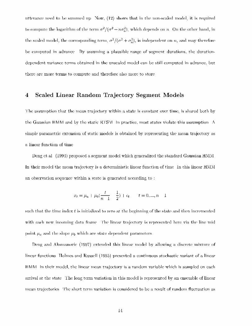
utterance need to be summed up. Now, (12) shows that in the non-scaled model, it is requiredto compute the logarithm of the term �2=(�2+n�2a), which depends on n. On the other hand, inthe scaled model, the corresponding term, �2=(�2 + �2a), is independent on n, and may thereforebe computed in advance. By assuming a plausible range of segment durations, the duration-dependent variance terms obtained in the unscaled model can be still computed in advance, butthere are more terms to compute and therefore also more to store.4 Scaled Linear Random Trajectory Segment ModelsThe assumption that the mean trajectory within a state is constant over time, is shared both bythe Gaussian HMM and by the static RTSM. In practice, most states violate this assumption. Asimple parametric extension of static models is obtained by representing the mean trajectory asa linear function of time.Deng et al. (1994) proposed a segment model which generalized the standard Gaussian HMM.In their model the mean trajectory is a deterministic linear function of time. In this linear HMMan observation sequence within a state is generated according to :xt = �a + �b( tn�1 � 12) + �t t = 0; :::; n � 1such that the time index t is initialized to zero at the beginning of the state and then incrementedwith each new incoming data frame. The linear trajectory is represented here via the line midpoint �a and the slope �b which are state dependent parameters.Deng and Aksmanovic (1997) extended this linear model by allowing a discrete mixture oflinear functions. Holmes and Russell (1995) presented a continuous stochastic variant of a linearHMM. In their model, the linear mean trajectory is a random variable which is sampled on eacharrival at the state. The long term variation in this model is represented by an ensemble of linearmean trajectories. The short term variation is considered to be a result of random uctuation as14

it is in the static case. In this model the segmented data is generated according to :xt = �a + a+ (�b + b)( tn�1 � 12) + �t t = 0; :::; n � 1where x0; :::; xn�1 is the observation sequence, �a and �b are �xed parameters , a and b areindependent normal random variables :a � N(0; �2a) ; b � N(0; �2b )and �t is a Gaussian white noise term, �t � N(0; �2). The line �a + �b( tn�1 � 12) is the averagetrajectory over all segment realizations and �a and �b de�ne a distribution function over all lineartrajectories. Denote, Fa(n) = n ; Fb(n) = n(n+1)12(n�1) = n�1Xt=0( tn�1 � 12) (21)Ea;x = 1Fa(n)Xt xt ; Eb;x = 1Fb(n)Xt xt( tn�1 � 12) (22)(a; b) = argmaxa;b f(x; a; b)In Appendix A we compute explicit expressions for a and b and prove that the true PDF f(x)and the MAP approximation f(x; a; b) are related viaf(x) = � 1�2a + Fa(n)�2 �� 12 1�2b + Fb(n)�2 !� 12 2�f(x; a; b)This relation corresponds to (13) in the static case.As in the static case, there is no closed form expression for the ML estimation of the linearmodel parameters. Holmes and Russell (1995) proposed an approximated solution which is anextension of their solution for the static RTSM. Alternatively, although the linear RTSM is out ofthe scope of dynamical system models, the EM approach for static RTSM, suggested by Digalakis(1992), can be generalized to the linear case. The missing data in the EM algorithm are thehidden values of the random variables a and b, which are sampled for each segment realization.15

The proposed EM algorithm is developed in Appendix B. The balancing problem, discussed inthe previous section, also exists in the linear model. The approach of using a Richter distributionfor better modeling the intra-segmental variability, was applied to the linear RTSM by Holmesand Russell (1997).We now present the scaled version of the linear RTSM. The motivation for this model issimilar to that for the static case. The scaled model spreads the information on the hidden lineartrajectory uniformly over time. The segment x is generated in the scaled model according to :xt = �a + a+ (�b + b)( tn�1 � 12) + �t t = 0; :::; n � 1The di�erence from the non-scaled linear model is that now the variances of a and b are dependenton segment duration as follows :a � N 0; �2aFa(n)! ; b � N 0; �2bFb(n)!The joint PDF of x, a and b is :f(x; a; b) = pFa(n)p2��a pFb(n)p2��b � 1p2���n e� 12g(x;a;b)where g(x; a; b) = Fa(n)a2�2a + Fb(n)b2�2b + 1�2 Xt (xt � (�a + a)� (�b + b)( tn�1 � 12))2Algebraic manipulation of g(x; a; b) reveals:(a; b) = argmaxa;b f(x; a; b) = E((a; b)jx) (23)= 0@ 1�2 Pt(xt � �a)Fa(n)( 1�2a + 1�2 ) ; 1�2 Pt(xt � �b( tn�1 � 12))( tn�1 � 12)Fb(n)( 1�2b + 1�2 ) 1ATo gain further insight to the probabilistic behavior of the model we derive an explicit expressionfor f(x). In Appendix A we have computed the following equivalent expression for g(x; a; b)g(x; a; b) = �Fa(n)�2a + Fa(n)�2 � (a� a)2 + Fb(n)�2b + Fb(n)�2 ! (b� b)2 + g(x; a; b) (24)16

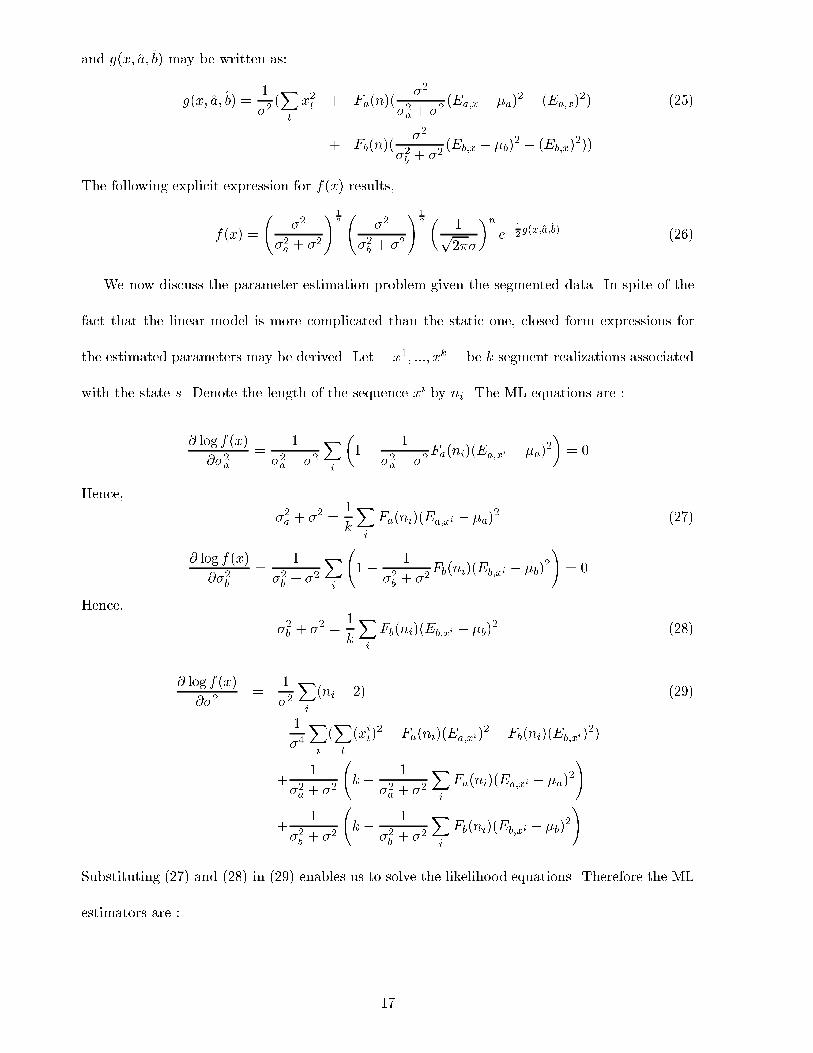
and g(x; a; b) may be written as:g(x; a; b) = 1�2 (Xt x2t + Fa(n)( �2�2a + �2 (Ea;x � �a)2 � (Ea;x)2) (25)+ Fb(n)( �2�2b + �2 (Eb;x � �b)2 � (Eb;x)2))The following explicit expression for f(x) results,f(x) = �2�2a + �2! 12 �2�2b + �2!12 � 1p2���n e� 12g(x;a;b) (26)We now discuss the parameter estimation problem given the segmented data. In spite of thefact that the linear model is more complicated than the static one, closed form expressions forthe estimated parameters may be derived. Let x1; :::; xk be k segment realizations associatedwith the state s. Denote the length of the sequence xi by ni. The ML equations are :@ log f(x)@�2a = 1�2a + �2 Xi �1� 1�2a + �2Fa(ni)(Ea;xi � �a)2� = 0Hence, �2a + �2 = 1kXi Fa(ni)(Ea;xi � �a)2 (27)@ log f(x)@�2b = 1�2b + �2 Xi 1� 1�2b + �2Fb(ni)(Eb;xi � �b)2! = 0Hence, �2b + �2 = 1kXi Fb(ni)(Eb;xi � �b)2 (28)@ log f(x)@�2 = 1�2 Xi (ni � 2) (29)� 1�4 Xi (Xt (xit)2 � Fa(ni)(Ea;xi)2 � Fb(ni)(Eb;xi)2)+ 1�2a + �2 k � 1�2a + �2 Xi Fa(ni)(Ea;xi � �a)2!+ 1�2b + �2 k � 1�2b + �2 Xi Fb(ni)(Eb;xi � �b)2!Substituting (27) and (28) in (29) enables us to solve the likelihood equations. Therefore the MLestimators are :17

�a = Pi Fa(ni)Ea;xiPi Fa(ni) = Pi;t xitPi Fa(ni)�b = Pi Fb(ni)Eb;xiPi Fb(ni) = Pi;t xit( tni�1 � 12)Pi Fb(ni)�2 = Pi(Pt(xit)2 � Fa(ni)(Ea;xi)2 � Fb(ni)(Eb;xi)2)Pi(ni � 2)�2a = 1kXi Fa(ni)(Ea;xi � �a)2 � �2�2b = 1kXi Fb(ni)(Eb;xi � �b)2 � �25 Experimental ResultsWe evaluated the model presented in the previous section using the ARPA, large vocabulary,speaker independent, continuous speech, Wall Street Journal (WSJ) corpus. Experiments wereconducted with DECIPHER, SRI's continuous speech recognition system (Digalakis, Monaco andMurveit, 1996). The recognizer was con�gured with a front-end that outputs a 39-dimensionalvector. The �rst components of the vector consist of 12 cepstral coe�cients and an energy term.The other components of the feature vector are the �rst and second time derivatives of the �rst13 components.The task we choose for evaluation is phonetic classi�cation. In classi�cation the correct seg-mentation (phone beginning and ending time) of the input observation sequence is given. Ourobjective is to assign correct phone labels to each segment. The DECIPHER system was usedto determine automatically the phone segmentation for each sentence in the database. Havingobtained phonetically aligned test data, the actual classi�cation process is just a matter of �ndingthe most likely phone label for a speech segment according to the models being evaluated. Thetraining set consists of 100 realizations in various contexts for each phone. The testing set consistsof another 100 realizations for each phoneme. 18

The goal of the experiments we have conducted is to compare between the performance ofthe scaled and unscaled random mean trajectory models. In previous sections we have discussedboth the cases of constant and linear mean trajectories. The experiments were performed forstatic as well as linear models. This enable us to �nd how much the assumption of linear meantrajectory improves the performance. We also add results for models where the mean trajectory isa deterministic parameter (i.e. standard Gaussian HMM and Deng's linear model) as a reference.It should be noted that a deterministic model has less parameters than the corresponding randommodel. The acoustic models we implemented for evaluation were:1. Standard Gaussian HMM.2. Static RTSM (Russell, 1993).3. Scaled static RTSM (presented in section 3).4. Linear mean trajectory segment model (Deng et al., 1994).5. Linear RTSM (Holmes and Russell, 1995).6. Scaled linear RTSM (presented in section 4).Several alternatives for model topologies were employed in order to analyze the balancingproblem in di�erent situations. The �rst analyzed topology assigns one segment to the entirephone. The second one still associates a single segment model with each phone, but includesself loops. In other words, the phone can be modeled by a number of segments which are allcorresponding to the same segmental model. The third topology, models each phone using threestates. The last examined topology is also a three state model but a skip over a state is allowed.In this manner a phone can be explained using at most three states. Note that in the secondand the forth topologies the number of segments per phone is not �xed. Balancing the modelcomponents in those cases is critical. 19

Training the models that include more than one segment per phone was done using the seg-mental K-means algorithm. The parameters of the unscaled random models were computed usingthe iterative inner EM algorithm that is presented in appendix B. We preferred to use this trainingmethod because, although it is an iterative procedure, it computes the true likelihood function.The scaled model was trained using the closed from formulae that were developed in previoussections. The random models, both scaled and unscaled, were initialized using the deterministicversion of the model for the �rst iteration of the segmental K-means algorithm. Duration was notmodeled explicitly. Therefore, all durations were assigned equal probability.(Table 1 should be placed about here )As can be seen, the scaled model usually outperforms the previously suggested non-scaledmodel, both for the static case and for the linear case. These results also reassess the signi�cantperformance improvement caused by using a linear model instead of a static one. It is noteworthyto mention that by comparing the parameters of the scaled and the corresponding unscaled model,we have found that the values of the mean parameters and the values of the intra-segmentalvariances are similar.Another task we evaluated is triphone classi�cation. Given a triphone context (the phonesbefore and after the current one), the goal is to determine the label of the current phone basedon the acoustics. Context dependent classi�cation was chosen because, in that case there arefewer discrepancies between utterances. Hence, in practice, this is usually the case of interestwhen using segment models. The topology we have used for this task is the simplest one. Eachphoneme is modeled by a single segmental model. This is the �rst topology from the topologieslist of the previous experiment.In Table 2 we present recognition results for some frequently occurring triphone contexts. The�rst column in Table 2 summarizes a classi�cation experiment given the triphone context m-n.The segmented WSJ database was used to extract the phones that appear between the phonesm and n. The classi�cation was done among those phonemes that have a signi�cant number of20

occurrences (at least 60) in the m-n context. In this context these phonemes are (using ARPABETnotation) : aa, ae, ah, aw, ax, ay, eh, ey and iy. Half of the data was used to train the triphonemodels. The other half was used for the actual classi�cation task. The subsequent four columnspresent results for similar classi�cation tasks in other triphone contexts. The �nal column presentsthe classi�cation performance averaged over the 120 most frequently occurring triphone contexts.As can be seen, the scaled model outperforms the previously suggested non scaled model.(Table 2 should be placed about here )6 ConclusionIn this study we have proposed, implemented and evaluated a new type of random trajectorysegment model where the variance of the mean trajectory is inversely proportional to the segmentduration. In this model the division of the acoustic information in an utterance does not dependon a speci�c segmentation. Instead, we extract the same amount of information about the meantrajectory from each data frame. We have named this approach a scaled RTSM. One desirableattribute of the scaled model is that it leads to a simple training algorithm. More precisely, given atraining set, consisting of a list of segment realizations, the ML estimation of the scaled model canbe solved analytically. On the other hand, in the non-scaled model, an iterative algorithm, (e.g.,EM) is required. Such an iterative algorithm, is not guaranteed to reach the global maximum.Appendix AWe derive an explicit expression for the PDF of the linear RTSM. Both the scaled and the non-scaled versions are discussed. We begin by analyzing the scaled model. The de�nition of thescaled linear model implies that the joint PDF of the observed segment x of length n and thelinear function coe�cients a and b is :21

f(x; a; b) = pFa(n)p2��a pFb(n)p2��b � 1p2���n e� 12g(x;a;b)where g(x; a; b) = Fa(n)a2�2a + Fb(n)b2�2b + 1�2 Xt (xt � (�a + a)� (�b + b)( tn�1 � 12))2We show that g(x; a; b) may be written as:g(x; a; b) = �Fa(n)�2a + Fa(n)�2 � (a� a)2 + Fb(n)�2b + Fb(n)�2 ! (b� b)2 +1�2 (Fa(n)( �2�2a + �2 (Ea;x � �a)2 � (Ea;x)2) +Fb(n)( �2�2b + �2 (Eb;x � �b)2 � (Eb;x)2) +Xt x2t )The terms a, b, Fa(n), Fb(n), Ea;x and Eb;x are de�ned in (21), (22).g(x; a; b) = Fa(n)a2�2a + Fb(n)b2�2b + 1�2 Xt (xt � (�a + a)� (�b + b)( tn�1 � 12))2= �Fa(n)�2a + Fa(n)�2 � a2 � 2a 1�2 Xt (xt � �a) + Fb(n)�2b + Fb(n)�2 ! b2 � 2b 1�2 Xt (xt � �b( tn�1 � 12))( tn�1 � 12) +1�2 Xt (xt � �a � �b( tn�1 � 12))2= �Fa(n)�2a + Fa(n)�2 � a� �2a�2a + �2 (Ea;x � �a)!2 + Fb(n)�2b + Fb(n)�2 ! b� �2b�2b + �2 (Eb;x � �b)!2�Fa(n)�2 �2a�2a + �2 (Ea;x � �a)2 � Fb(n)�2 �2b�2b + �2 (Eb;x � �b)2 +1�2 Xt (xt � �a � �b( tn�1 � 12))2 (30)Given the observation sequence x, g(x; a; b) is a quadratic form in a and b. Hence, we concludethat the conditional distribution of a and b given the segment x is Gaussian. Furthermore, a andb are conditionally independent. Now, the �rst moments may be read directly from (30):22

E(ajx) = a = �2a�2a + �2! (Ea;x � �a)V ar(ajx) = �Fa(n)�2a + Fa(n)�2 ��1E(bjx) = b = �2b�2b + �2! (Eb;x � �b)V ar(bjx) = Fb(n)�2b + Fb(n)�2 !�1Direct algebraic manipulations reveal the following relationXt (xt � �a � �b( tn�1 � 12))2 =Fa(n)((Ea;x � �a)2 � (Ea;x)2) + Fb(n)((Eb;x � �b)2 � (Eb;x)2) +Xt x2tSubstituting this relation in (30) yields :g(x; a; b) = �Fa(n)�2a + Fa(n)�2 � (a� a)2 + Fb(n)�2b + Fb(n)�2 ! (b� b)2 +1�2 (Xx2t + Fa(n) (1� �2a�2a + �2 )(Ea;x � �a)2 � (Ea;x)2!+Fb(n) (1� �2b�2b + �2 )(Eb;x � �b)2 � (Eb;x)2!)Hence, g(x; a; b) = �Fa(n)�2a + Fa(n)�2 � (a� a)2 + Fb(n)�2b + Fb(n)�2 ! (b� b)2 + g(x; a; b)Now, g(x; a; b) may be written as :g(x; a; b) = 1�2 (Xt x2t + Fa(n)( �2�2a + �2 (Ea;x � �a)2 � (Ea;x)2)+ Fb(n)( �2�2b + �2 (Eb;x � �b)2 � (Eb;x)2))Using this representation we may solve the double integral :f(x) = Za Zb f(x; a; b)da dband obtain the following explicit expression for the PDF,f(x) = �Fa(n)�2a + Fa(n)�2 �� 12 Fb(n)�2b + Fb(n)�2 !� 12 2�f(x; a; b)23

= �2�2a + �2! 12 �2�2b + �2! 12 � 1p2���n e� 12 g(x;a;b)The expressions we derived for f(x), g(x; a; b) and the moments of the conditional distributionof a and b given xmay be easily transformed to the non-scaled linear case. We need only substituteFa(n)�2a and Fb(n)�2b for �2a and �2b . For example, in the non-scaled case we have :E(ajx) = a = Fa(n)�2aFa(n)�2a + �2! (Ea;x � �a)E(bjx) = b = Fb(n)�2bFb(n)�2b + �2! (Eb;x � �b)and the PDF of the observation sequence x of length n is :f(x) = � 1�2a + Fa(n)�2 �� 12 1�2b + Fb(n)�2 !� 12 2�f(x; a; b)Appendix BThe static RTSM can be seen as a special case of the dynamical system model studied by Digalakis(1992) such that the state space is constant over time. The EM algorithm presented by Digalakis(1992) can be applied to the static RTSM. In this appendix we derive the EM re-estimationequations for the unscaled linear RTSM which is out of the scope of dynamical system models.The re-estimation equations for static RTSM can be easily deduced from the equations developedhere. Suppose we have k segment realizations x1; :::; xk. Denote the length of xi by ni. Denoteby ai and bi the hidden coe�cients of the line which was sampled for the segment xi. De�nezi = (xi; ai; bi), z1; :::; zk are the complete data for this EM framework. Denote the parameterset we want to estimate by � = f�a; �b; �2a; �2b ; �2g. The current estimate at the beginning of theiteration is denoted by �0 = f�a0; �b0; �2a0; �2b0; �20g.log f(zi; �) = log �2a + a2i�2a + log �2b + b2i�2b + ni log �2 +24

1�2 Xt (xit � (�a � ai)� (�b � bi)( tn�1 � 12))2 + Cwhere C is a constant that is independent of the parameter vector �. Hence,E(log f(zi; �)jx; �0) = ni log �2+log �2a + 1�2aE(a2i jxi; �0) + log �2b + 1�2b E(b2i jxi; �0)++ 1�2 Xt E((xit � (�a � ai)� (�b � bi)( tni�1 � 12))2jxi; �0)Denote : Eai = E(aijxi; �0) = � 1�2a0 + Fa(ni)�20 ��1 Fa(ni)�20 (Ea;xi � �a0)Vai = V ar(aijxi; �0) = � 1�2a0 + Fa(ni)�20 ��1Ebi = E(bijxi; �0) = 1�2b0 + Fb(ni)�20 !�1 Fb(ni)�20 (Eb;xi � �b0)Vbi = V ar(bijxi; �0) = 1�2b0 + Fb(ni)�20 !�1where Fa(ni) = ni ; Ea;xi = 1Fa(ni)Xt xitFb(ni) = ni(ni+1)12(ni�1) ; Eb;xi = 1Fb(ni)Xt xit( tni�1 � 12)These relations are developed in Appendix A. Direct algebraic manipulations reveal the followingrelation : E((xit � (�a � ai)� (�b � bi)( tni�1 � 12))2jxi; �0) =Fa(ni)Vai + Fb(ni)Vbi +Xt (xit � (�a +Eai)� (�b +Ebi)( tni�1 � 12))225

We now de�ne the EM auxiliary function :Q(�; �0) = E(log f(z; �)jx; �0) =Xi E(log f(zi; �)jxi; �0)= k log �2a + 1�2a Xi E(a2i jxi; �0) + 1�2 Xi Fa(ni)Vai +k log �2b + 1�2b Xi E(b2i jxi; �0) + 1�2 Xi Fb(ni)Vbi +Xi ni log �2 + 1�2 Xi;t (xit � (�a +Eai)� (�b +Ebi)( tni�1 � 12))2Optimization of the auxiliary function with respect to the model parameters yields the follow-ing new estimated parameter vector (this optimization is carried out by setting the correspondingpartial derivatives to zero).�a = Pi Fa(ni)(Ea;xi �Eai)Pi Fa(ni)�b = Pi Fb(ni)(Eb;xi �Ebi)Pi Fb(ni)�2a = 1kXi (Vai +E2ai) = 1k Xi E(a2i jxi; �0)�2b = 1kXi (Vbi +E2bi) = 1kXi E(b2i jxi; �0)�2 = 1Pi ni Xi (Fa(ni)Vai + Fb(ni)Vbi +Xt (xit � (�a +Eai)� (�b +Ebi)( tni�1 � 12))2)ReferencesDempster, A. P., Laird, N. M. & Rubin, D. B. (1977). Maximum likelihood estimation fromincomplete data, Journal of the Royal Statistics Society, 39, 1-38.Deng, L., Aksmanovic, M., Sun, D. & Wu, J. (1994). Speech recognition using hidden Markovmodels with polynomial regression functions as non stationary states, IEEE Transactions onSpeech and Audio Processing 2, 507-520.Deng, L. & Aksmanovic, M. (1997). Speaker independent phonetic classi�cation using hidden26

Markov models with state conditioned mixtures of trend functions, IEEE Transactions on Speechand Audio Processing, 5, 319-324.Digalakis, V., Rohlicek, J. & Ostendorf, M. R. (1993). A dynamical system approach tocontinuous speech recognition. IEEE Transactions on Speech and Audio Processing, 1, 431-442.Digalakis, V. (1992). Segment-based stochastic models of spectral dynamics for continuousspeech recognition, Ph.D Thesis, Boston University.Digalakis, V., Monaco, P. & Murveit, H. (1996). Genones: generalized mixture tying incontinuous hidden Markov model-based speech recognizers, IEEE Transactions on Speech andAudio Processing 4, 281-289.Gales, M. & Young, S. (1993). The theory of segmental hidden Markov models, TechnicalReport CUED/F-INFENG/TR 133, Cambridge, U.K.Ghitza, O. & Sondhi, M. (1993). Hidden Markov models with templates as non-stationarystates: an application to speech recognition, Computer Speech and Language 7, 101-119.Goldberger, J., Burshtein, D. & Franco, H. (1997). Segmental modeling using a continuousmixture of non-parametric models, submitted for publication.Holmes, W. & Russell, M. (1995). Speech recognition using a linear dynamic segmental HMMs,Proc. Eurospeech, pp. 1611-1614.Holmes, W. & Russell, M. (1996). Modeling speech variability with segmental HMMs, Proc.Int. Conf. Acoustics, Speech and Signal Processing, 447-450.Holmes, W. & Russell, M. (1997). Linear dynamic segmental HMMS : Variability repre-sentation and training procedure, Proc. Int. Conf. Acoustics, Speech and Signal Processing,1399-1402.Juang, B. H. & Rabiner, L. R. (1990). The segmental K-means algorithm for estimating pa-rameters of hiddenMarkov models, IEEE Transactions on Acoustics, Speech and Signal Processing38, 1639-1641.Ostendorf, M., Digalakis, V. & Kimball, O. A. (1996). From HMMs to segment models: a27

uni�ed view of stochastic modeling for speech recognition, IEEE Transactions on Speech andAudio Processing 4, 360-377.Russell, M. (1993). A segmental HMM for speech pattern modeling, Proc. Int. Conf. Acous-tics, Speech and Signal Processing, 499-502.

28

AcknowledgmentWe acknowledge the speech group at SRI international for providing us segmented data obtainedby using the DECIPHER speech recognition system.

29

model one state one state three states three statesself-loop with skipsdeterministic 52.1 61.7 61.9static non-scaled 50.7 52.4 61.1 61.7scaled 51.5 55.1 62.3 62.8deterministic 57.2 57.8 61.8 62.3linear non-scaled 58.0 57.0 63.3 63.9scaled 59.1 58.1 62.2 64.1Table 1: Phoneme classi�cation rate results

model m-?-n p-?-t s-?-ae t-?-s k-?-t averagestatic non-scaled 49.4 61.0 80.3 69.3 82.9 79.6scaled 52.7 65.1 79.6 71.4 84.2 80.3linear non-scaled 59.3 64.0 88.4 72.1 87.5 82.0scaled 61.9 67.7 88.9 74.8 90.0 82.4Table 2: Triphone classi�cation rate results30

3 4 5 6 7 8 90

5

10

15

20

25

30

35

40

segment length

recip

roca

l of v

arian

ce

Figure 1: The reciprocal of the variance of the sampled mean trajectory as a function of thesegment length, for the �rst seven mel-cepstrum features, based on 750 realizations of the phoneme`t' in the triphone context `s-t-ih'.

31