11

Identifying ARIMA ModelsIdentifying ARIMA Models

What you need to knowWhat you need to know

22

Autoregressive of the second orderAutoregressive of the second order

• X(t) = b1 x(t-1) + b2 x(t-2) + wn(t)

• b2 is the partial regression coefficient measuring the effect of x(t-2) on x(t) holding x(t-1) constant

• Since x(t) is regressed on itself lagged, b2

can also be interpreted as a partial autoregression coefficient of x(t) regressed on itself lagged twice.

33

continuedcontinued• In one more step b2 can be defined as the

partial autocorrelation coefficient at lag 2, b2 = pacf(2)

• Solving the yule-Walker equations:

• b2 = {acf(2) – [acf(1)]2 }/[1 – [acf(1)]2

• We know that if the process is autoregressive of the first order, then acf(2) = [acf(1)]2 and so b2 = 0

44

So now we are back to So now we are back to autoregressive of the first oderautoregressive of the first oder

• x(t) = b x(t-1) + wn(t)

• There is only one regression coefficient, b, so acf(1) = pacf(1) = b

55

In summaryIn summary• The partial autocorrelation function, pacf(u)

indicates the order of the autregressive process. If only pacf(1) is significantly different from zero, then the autoregressive process is of order one. If the pacf(2) is significantly different from zero, then the autoregressive process is of order two, and so on.

• Thus we use the partial autocorrelation function to specify the order of the autoregressive process to be estimated

66

The autocorrelation functionThe autocorrelation function

• The autocorrelation function, acf(u) is used to determine the order of the moving average process

• If acf(1) is significantly different from zero and there are no other significant autocorrelations, then we specify a first order MA process to be estimated

77

Cont.Cont.

• If there is a significant autocorrelation at lag two and none at higher lags, then we specify a second order moving average process

88

Moving Average ProcessMoving Average Process

• X(t) = wn(t) + a1wn(t-1) + a2wn(t-2) + a3wn(t-3)

• Taking expectations the mean function is zero, Ex(t) = m(t) = o

• Multiplying by x(t-1) and taking expectations, E[x(t)x(t-1)] =

• EX(t) = wn(t) + a1wn(t-1) + a2wn(t-2) + a3wn(t-3)

X(t-1) = wn(t-1) + a1wn(t-2) + a2wn(t-3) + a3wn(t-4), γx,x (1) = [a1 + a1 a2 + a2 a3 ] σ2

99

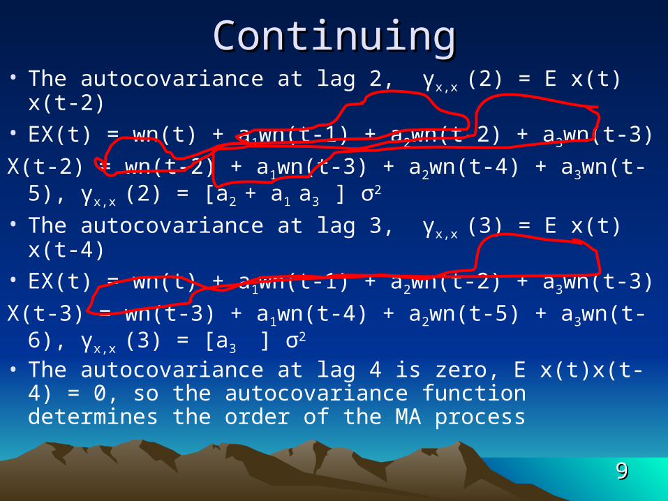
ContinuingContinuing• The autocovariance at lag 2, γx,x (2) = E x(t) x(t-2)• EX(t) = wn(t) + a1wn(t-1) + a2wn(t-2) + a3wn(t-3)

X(t-2) = wn(t-2) + a1wn(t-3) + a2wn(t-4) + a3wn(t-5), γx,x (2) = [a2 + a1 a3 ] σ2

• The autocovariance at lag 3, γx,x (3) = E x(t) x(t-4)• EX(t) = wn(t) + a1wn(t-1) + a2wn(t-2) + a3wn(t-3)

X(t-3) = wn(t-3) + a1wn(t-4) + a2wn(t-5) + a3wn(t-6), γx,x (3) = [a3 ] σ2

• The autocovariance at lag 4 is zero, E x(t)x(t-4) = 0, so the autocovariance function determines the order of the MA process

1010

Specifying ARMA ProcessesSpecifying ARMA Processes• x(t) = A(z)/B(z)• The autocovariance function divided by the variance,

i.e. the autocorrelation function, acf(u), indicates the order of A(z) and the partial autocorrelation function, pacf(u) indicates the order of B(z)

• In Eviews specify x(t) c ar(1) ar(2) ….ar(u) for a u th order B(z) and include ma(1) ma(2) ….ma(u) for a uth order A(z),

• i.e. X(t) c ar(1) ar(2) …ar(u) ma(1) ma(2) …ma(u)

1111

Summary of IdentificationSummary of Identification• Spreadsheet

• Trace: Is it stationary?

• Histogram: is it normal?

• Correlogram: order of A(z) and B(z)

• Unit root test: is it stationary?1111

• Specification

• estimation

1212

ARMA ProcessesARMA Processes• Identification• Specification and Estimation• Validation

– Significance of estimated parameters and DW– Actual, fitted and residual– Residual tests

• Correlogram: are they orthogonal? Also the Breusch-Godfrey test for serial correlation

• Histogram; are they normal?

• Forecasting

1313

Example: Capacity utilization mfg.Example: Capacity utilization mfg.

1414

SpreadsheetSpreadsheet

1515

HistogramHistogram

0

10

20

30

40

50

60

66 68 70 72 74 76 78 80 82 84 86 88

Series: MCUMFNSample 1972:01 2010:03Observations 459

Mean 78.98322Median 79.30000Maximum 88.50000Minimum 65.20000Std. Dev. 4.647918Skewness -0.603442Kurtosis 3.051589

Jarque-Bera 27.90780Probability 0.000001

1616

CorrelogramCorrelogram

1717

Unit root testUnit root test

1818

Pre-WhitenPre-Whiten

Gen dmcumfn =mcumfn – mcumfn(-1)

1919

SpreadsheetSpreadsheet

2020

TraceTrace

-4

-3

-2

-1

0

1

2

75 80 85 90 95 00 05 10

DMCUMFN

2121

histogramhistogram

0

20

40

60

80

100

120

-4 -3 -2 -1 0 1 2

Series: DMCUMFNSample 1972:02 2010:03Observations 458

Mean -0.023799Median 0.000000Maximum 1.800000Minimum -3.900000Std. Dev. 0.660698Skewness -1.109196Kurtosis 7.351042

Jarque-Bera 455.1915Probability 0.000000

2222

CorrelogramCorrelogram

2323

Unit root testUnit root test

2424

SpecificationSpecification

Dmcumfn c ar(1) ar(2)

2525

Estimation

2626

ValidationValidation

-4

-2

0

2

4

-4

-2

0

2

75 80 85 90 95 00 05 10

Residual Actual Fitted

2727

Correlogram of the residualsCorrelogram of the residuals

2828

Breusch-Godfrey Serial correlation testBreusch-Godfrey Serial correlation test

2929

Re-SpecifyRe-Specify

3030

EstimationEstimation

3131

ValidationValidation

-4

-2

0

2

4

-4

-2

0

2

75 80 85 90 95 00 05 10

Residual Actual Fitted

3232

Correlogram of the ResidualsCorrelogram of the Residuals

3333

Breusch-Godfrey Serial correlation testBreusch-Godfrey Serial correlation test

3434

Histogram of the residualsHistogram of the residuals

0

20

40

60

80

100

-3 -2 -1 0 1 2

Series: ResidualsSample 1972:05 2010:03Observations 455

Mean 8.09E-05Median 0.010460Maximum 2.669327Minimum -2.954552Std. Dev. 0.583609Skewness -0.316126Kurtosis 6.875041

Jarque-Bera 292.2558Probability 0.000000

3535

Forecasting: Procs. Workfile rangeForecasting: Procs. Workfile range

3636

Forecasting: Equation Forecasting: Equation window.forecastwindow.forecast

3737

ForecastingForecasting

-1.5

-1.0

-0.5

0.0

0.5

1.0

1.5

2.0

10:04 10:05 10:06 10:07 10:08 10:09 10:10 10:11 10:12

DMCUMFNF ± 2 S.E.

3838

Forecasting: Quick, showForecasting: Quick, show

3939

ForecastingForecasting

4040

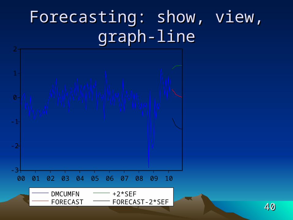
Forecasting: show, view, graph-lineForecasting: show, view, graph-line

-3

-2

-1

0

1

2

00 01 02 03 04 05 06 07 08 09 10

DMCUMFNFORECAST

+2*SEFFORECAST-2*SEF

4141

ReintegrationReintegration

4242

Forecasting mcumfnForecasting mcumfn

4343

Forecast mcumfn, quick, showForecast mcumfn, quick, show

4444

Forecasting mcumfnForecasting mcumfn

64

68

72

76

80

84

00 01 02 03 04 05 06 07 08 09 10

MCUMFNMCUMFNF

MCUMFNF+2*SEFMCUMFNF-2*SEF

4545

What can we learn from this forecast?What can we learn from this forecast?• If, in the next nine months, mcumfn grows

beyond the upper bound, this is new information indicating a rebound in manufacturing

• If, in the next nine months, mcumfn stays within the upper and lower bounds, then this means the recovery remains sluggish

• If mcumfn goes below the lower bound, run for the hills!