- 1 -

1 HYDROLOGY AND WATER RESOURCES Hydrology is the science that describes the occurrence of water on our planet and the processes that drive the circulation of the water between different stocks and locations where the water resides. When we use the words "water resources" we implicitly refer to the use that is made of the water, for whatever function. A resource is an input into some process of use, be it consumptive or non-consumptive. When we use the word resource, we imply a use or a function. Hence hydrology describes the occurrence and circulation of water, whereas water resources refer to the availability of water. Obviously the two are closely linked. The origin of all terrestrial water resources is the rainfall. In that sense, rainfall is the most important water resource of all. Sections 1.1 and 0 deal with the origin and occurrence of rainfall, and hence deal with hydrology. Subsequently, sections 1.3 and 1.4 deal with water resources and water balances, in relation to the potential water use.

1.1 Precipitation, the origin of all water resources

1.1.1 The atmosphere The lower layer of the atmosphere, up to a height of approximately 10 km, known as the troposphere, is the most interesting part from a hydrological point of view as it contains almost all of the atmospheric moisture. The percentage of water in moist air is usually less than 4 %. The composition of dry air is given in Table 1.1. Table 1.1: Composition of dry air

Mass % Volume % Nitrogen N2 75.5 78.1 Oxygen O2 23.1 20.9 Argon A 1.3 0.9

Others 0.1 0.1 The atmosphere depends for its heat content on the radiant energy from the sun. The atmosphere directly absorbs about one-sixth of the available solar energy, more than one third is reflected into space and less than one half is absorbed by the earth's surface. Heat from the earth's surface is released to the atmosphere by conduction (action of molecules of greater energy on those of less), convection (vertical interchange of masses of air) and radiation (long wave radiation). The process of conduction does not play a significant role. Radiation is an important link in the energy balance of the atmosphere. The "greenhouse effect", the increase of the atmospheric temperature as a result of a decrease in the long wave radiation, has grown into a worldwide concern. It is believed that man-produced gasses such as CO2, CH4 and N2O obstruct the outgoing radiation, gradually leading to an accumulation of energy and hence a higher atmospheric temperature.

- 2 -

ea-ed

Convection involves the vertical interchange of masses of air. The process is usually described assuming a parcel of air with approximate uniform properties, moving vertically without mixing with the surroundings. When a parcel of air moves upward it expands due to a decrease of the external pressure. The energy required for the expansion causes the temperature to fall. If the heat content of the air parcel remains constant, which is not uncommon (the parcel is transparent and absorbs little radiant heat), the conditions are called adiabatic. The rate of change of air temperature

with height is known as the lapse rate. The average lapse rate is 0.65 °C per 100 m rise and varies from 1.0 under dry-adiabatic conditions to 0.56 under saturated-adiabatic conditions. The lower value for the lapse rate of saturated air results from the release of latent heat due to condensation of water vapour. Its value depends on the air temperature. The pressure of the air is often specified in mbar and generally taken equal to 1013 mbar or 1.013 bar at mean sea level. In this note the SI unit for pressure Pa (Pascal) will be used, where 1000 mbar = 1 bar = 100,000 Pa = 100 kPa. Hence the pressure at mean sea level is taken as 101.3 kPa. The atmospheric pressure decreases with the height above the surface. For the lower atmosphere this rate is approximately 10 kPa per kilometre. The water vapour content of the air, or humidity, is usually measured as a water vapour pressure (kPa). The water vapour pressure at which the air is saturated with water vapour, the saturation vapour pressure of the air, ea is related to the temperature of the air as shown in Figure 1.1. If a certain mass of air is cooled while the vapour pressure remains constant; the air mass becomes saturated at a temperature known as dewpoint temperature, Td. The corresponding actual or dewpoint vapour pressure of the air mass is indicated by ed. The vapour pressure deficit is defined as the difference between the actual vapour pressure and the saturation vapour pressure that applies for the prevailing air temperature Ta, thus (ea - ed). The relative humidity of the air is the ratio of actual and saturation vapour pressure, or when expressed as percentage:

= 100d

a

eRHe

Equation 1.1

Figure 1.1: Relation between saturation vapour pressure ea and air temperature Ta

- 3 -

1.1.2 Formation of precipitation The conditions for precipitation to take place may be summarized stepwise as follows: a supply of moisture b cooling to below point of condensation c condensation d growth of particles The supply of moisture is obtained through evaporation from wet surfaces, transpiration from vegetation or transport from elsewhere. The cooling of moist air may be through contact with a cold earth surface causing dew, white frost, mist or fog, and loss of heat through long wave radiation (fog patches). However, much more important is the lifting of air masses under adiabatic conditions (dynamic cooling) causing a fall of temperature to near its dew point. Five lifting mechanisms can be distinguished: 1. Convection, due to vertical instability of the air. The air is said to be unstable if

the temperature gradient is larger than the adiabatic lapse rate. Consequently a parcel moving up obtains a temperature higher than its immediate surroundings. Since the pressure on both is the same the density of the parcel becomes less than the environment and buoyancy causes the parcel to ascend rapidly. Instability of the atmosphere usually results from the heating of the lower air layers by a hot earth surface and the cooling of the upper layers by outgoing radiation. Convective rainfall is common in tropical regions and it usually appears as a thunderstorm in temperate climates during the summer period. Rainfall intensities of convective storms can be very high locally; the duration, however, is generally short.

2. Orographic lifting. When air passes over a mountain it is forced to rise which may

cause rainfall on the windward slope. As a result of orographic lifting rainfall amounts are usually highest in the mountainous part of the river basin.

3. Frontal lifting. The existence of an area with low pressure causes surrounding air to move into the depression, displacing low pressure air upwards, which may then be cooled to dew point. If cold air is replaced by warm air (warm front) the frontal zone is usually large and the rainfall of low intensity and long duration. A cold front shows a much steeper slope of the interface of warm and cold air usually resulting in rainfall of shorter duration and higher intensity (see Figure 1.2). Some depressions are died-out cyclones.

4. Cyclones, tropical depressions or hurricanes. These are active depressions

which gain energy while moving over warm ocean water and which dissipate energy while moving over land or cold water. They may cause torrential rains and heavy storms. Typical characteristics of these tropical depressions are high intensity rainfall of long duration (several days). Notorious tropical depressions occur in the Caribbean (hurricanes), the Bay of Bengal (monsoon depressions), the Far East (typhoons), Southern Africa (cyclones), and on the islands of the Pacific (cyclones, willy-willies). This group of depressions is quite different in character from other lifting mechanisms; data on extreme rainfall originating from cyclones should be treated separately from other rainfall data, as they belong to a different statistical population. One way of dealing with cyclones is through mixed distributions (see section 1.2.2).

- 4 -

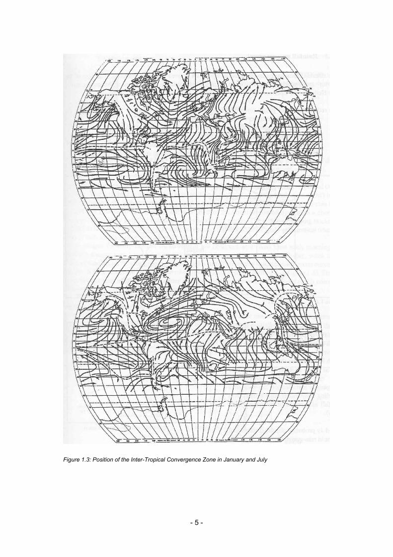
5. Convergence. The Inter-Tropical Convergence Zone is the tropical region where the air masses originating from the Tropics of Cancer and Capricorn converge and lift. In the tropics, the position of the ITCZ governs the occurrence of wet and dry seasons. This convergence zone moves with the seasons. In July, the ITCZ lies to the North of the equator and in January it lies to the South (see Figure 1.3). In the tropics the position of the ITCZ determines the main rain-bringing mechanism which is also called monsoon. Hence, the ITCZ is also called the Monsoon Trough, particularly in Asia. In certain places near to the equator, such as on the coast of Nigeria, the ITCZ passes two times per year, causing two wet seasons; near the Tropics of Capricorn and Cancer (e.g. in the Sahel), however, there is generally only one dry and one wet season.

Figure 1.2: Frontal lifting

Condensation of water vapour into small droplets does not occur immediately when the air becomes saturated. It requires small airborne particles called aerosols which act as nuclei for water vapour to condense. Nuclei are salt crystals from the oceans, combustion products, dust, ash, etc. In the absence of sufficient nuclei the air becomes supersaturated. When the temperature drops below zero, freezing nuclei with a structure similar to ice are needed for condensation of water vapour into ice crystals. These nuclei are often not available and the droplets become super-cooled to a temperature of -40 °C. Cloud droplets with a diameter of 0.01 mm need an up draught of only 0.01 m/s to prevent the droplet from falling. A growth of particles is necessary to produce precipitation. This growth may be achieved through coalescence, resulting from collisions of cloud droplets. Small droplets moving upwards through the clouds collide and unite with larger droplets which have a different velocity or move downwards. Another method of growth known as the Bergeron process is common in mixed clouds which consist of super-cooled water droplets and ice crystals. Water vapour condenses on the ice crystals, the deficit being replenished by the evaporation of numerous droplets. In the temperature range from -12 °C to -30 °C the ice crystals grow rapidly and fall through the clouds. Aggregates of many ice crystals may form snow flakes. Depending on the temperature near the surface they may reach the ground as rain, snow, hail or glazed frost.

- 5 -

Figure 1.3: Position of the Inter-Tropical Convergence Zone in January and July

- 6 -

1.1.3 Rainfall measurements The standard rain gauge as depicted in Figure 1.4 is used for daily readings. The size of the aperture and the height varies between countries but is usually standardized within each country (the Netherlands: aperture 200 (cm)2 (or 0.02 m2), height 40 cm). The requirements for gauge construction are: 1. The rim of the collector should have a sharp edge. 2. The area of the aperture should be known with an accuracy of 0.5 %. 3. Design is such that rain is prevented from splashing in or out. 4. The reservoir should be constructed so as to avoid evaporation. 5. In some climates the collector should be deep enough to store one day’s snowfall

Wind turbulence affects the catch of rainfall. Experiments in the Netherlands using a 400 (cm)2 rain gauge have shown that at a height of 40 cm the catch is 3-7% less than at ground level and as much as 4-16% at a height of 150 cm. Tests have shown that rain gauges installed on the roof of a building may catch substantially less rainfall as a result of turbulence (10-20%). Wind is probably the most important factor in rain-gauge accuracy. Updrafts resulting from air moving up and round the instrument reduce the rainfall catch. Figure 1.5 shows the

effect of wind speed on the catch according to Larson & Peck (1974). To reduce the effects of wind, rain gauges can be provided with windshields. Moreover, obstacles should be kept far from the rain gauge (distance at least twice the height of such an

Figure 1.4: Rain gauges

Figure 1.5: Effect of wind speed on rain catch

- 7 -

object) and the height of the gauge should be minimized (e.g. ground-level rain-gauge with screen to prevent splashing).

Recording gauges are of three different types: the weighing type, the tilting bucket type and the float type. The weighing type observes precipitation directly when it falls (including snow) by recording the weight of the reservoir e.g. with a pen on a chart. With the float type the rain is collected in a float chamber. The vertical movement of the float is recorded by pen on a chart. Both types have to be emptied manually or

by automatic means. The tilting or tipping bucket type

(Figure 1.4) is a very simple recording rain gauge, but less accurate (only registration when bucket is full, losses during tipping and losses due to evaporation). Storage gauges for daily rainfall measurement are observed at a fixed time each morning. Recording gauges may be equipped with charts that have to be replaced every day, week or month, depending on the clockwork. The rainfall is usually recorded cumulatively (mass curve) from which the hyetograph (a plot of the rainfall with time) is easily derived (see Figure 1.6). The tipping bucket uses an electronic counter or magnetic tape to register the counts (each count corresponds to 0.2 mm), for instance, per 15 minutes time interval.

Rainfall measurement by radar and satellite Particularly in remote areas or in areas where increased spatial or time resolution is required radar and satellite measurement of rainfall can be used to measure rainfall. Radar works on the basis of the reflection of an energy pulse transmitted by the radar which can be elaborated into maps that give the location (plan position indicator, PPI) and the height (range height indicator, RHI) of the storms (see Figure 1.7, after Bras, 1990).

A technology which has a large future is rainfall monitoring through remote sensing by satellite. Geostationary satellites, that orbit at the same velocity as the earth's rotation, are able to produce a film of weather development with a time interval

Figure 1.6: Hyetograph and corresponding mass curve

Figure 1.7: Forms of radar display: PPI (left) and RHI (right)

Hyetograph

Prec

ipita

tion

inm

m/h

our

- 8 -

between observations of several minutes. The resolution of the images is in the order of one km. This allows monitoring closely the development of convective storms, depressions, fronts, orographic effects and tropical cyclones. Successful efforts have been made to correlate rainfall with Cold Cloud Coverage (CCC) and Cold Cloud Duration (CCD) through simple mathematical regression. Particularly in remote areas the benefits of such methods are obvious.

Parameters defining rainfall When discussing rainfall data the following elements are of importance: 1. Intensity or rate of precipitation: the depth of water per unit of time in m/s,

mm/min, or inches/hour (see section 1.1.4). 2. Duration of precipitation in seconds, minutes or hours (see section 1.1.4). 3. Depth of precipitation expressed as the thickness of a water layer on the surface

in mm or inches (see section 1.1.4). 4. Area, that is the geographic extent of the rainfall in (km)2 or Mm2 (see section

1.1.5). 5. Frequency of occurrence, usually expressed by the 'return period' e.g. once in 10

years (see section 1.2.1).

1.1.4 Intensity, duration and rainfall depth We have seen that rainfall storms can be distinguished by their meteorological characteristics (convective, orographic, frontal, cyclonic). Another way to characterize storms is from a statistical point of view. Distinction is made between "interior" and "exterior" statistics: • exterior statistics refer to total

depth of the storm, duration of the storm, average intensity of the storm and time between storms;

• interior statistics refer to the time and spatial distribution of rainfall rate within storms.

The exterior statistics can generally be described by probabilistic distributions, which can be seasonally and spatially dependent. They are generally not statistically independent. Depth is related to duration: a long duration is associated with a large depth; average intensity is related to short duration. Moreover there is spatial correlation between points. With regard to storm interior, Eagleson (1970) observed that for given locations and climatic conditions some type of storms gave similar histories of rainfall accumulation. The percentage-mass curve of Figure 1.8 shows how typical curves are obtained for thunderstorms (convective storms) and cyclonic storms. The derivative (slope) of these curves is a graph for the rainfall intensity over time. Such a graph is referred to as the hyetograph and is usually presented in histogram form (see Figure 1.6). It can be seen from Figure 1.8 that convective storms have more or

Figure 1.8: Typical percentage mass curves of rainfall for thunderstorms and cyclones

- 9 -

less triangular (mound like) hyetographs with the highest intensity at the beginning of the storm (a steep start), whereas tropical cyclones have a bell-shaped hyetograph with the largest intensity in the middle of the storm. It should be observed that tropical cyclones have a much longer storm duration and a much larger rainfall depth than thunderstorms.

Another interior characteristic of a storm is the spatial distribution. The spatial distribution of a storm generally concentrates around one or two centres of maximum depth. The total depth of point rainfall distributed over a given area is a decreasing function of the distance from the storm centre. One can draw lines of equal rainfall depth around the centres of maximum depth (isohyets). When two rainfall stations are closely together, data from these stations may show a good

correlation. The further the stations lay apart, the smaller the chances of coincidence become. In general, correlation is better when the period of observation is larger. For a given period of observation, the correlation between two stations is defined by the correlation coefficient ∆ (–1<∆<1). The square of ∆ is known as the coefficient of determination (∆2). If there is no correlation, ∆ is near to zero, if the correlation is perfect, ∆=1. It is defined by:

ρσ σ

=cov( , )

( ) ( )x y

x y Equation 1.2

Table 1.2: Typical spatial correlation structure for different storm types

For a number of stations in a certain area the correlation coefficient can be determined pair-wise. In general, the larger the distance, the smaller the correlation will be. If r is defined as the distance between stations, then the correlation between stations at a distance r apart is often described by Kagan's formula:

ρ ρ= −0 0( ) exp( / )r r r Equation 1.3

This is an exponential function which equals ∆0 at r=0 and which

decreases gradually as r goes to infinity. The distance r0 is defined as the distance where the tangent at x=0 intersects the x-axis (see Figure 1.9). For convective storms, the steepness is very large and the value of r0 is small; for frontal or orographic rains, the value is larger. Also the period considered is reflected in the

Figure 1.9: Spatial correlation of daily rainfalls

Period 1 hour Period 1 day Period 1

month Rain type r0

(km) ρ0 r0

(km) ρ0 r0

(km) ρ0

Very local

convec-tive

5 0.8 10 0.88 50 0.95

Mixed convec-

tive orogra-

phic

20 0.85 50 0.92 1500 0.98

Frontal rains from

depres-sions

100 0.95 1000 0.98 5000 0.99

- 10 -

steepness; for a short period of observation r0 is small. Table 1.2 gives indicative values of r0 and ∆0.

1.1.5 Areal rainfall In general, for engineering purposes, knowledge is required of the average rainfall depth over a certain area: the areal rainfall. Some cases where the areal rainfall is required are: design of a culvert or bridge draining a certain catchment area, design of a pumping station to drain an urbanized area; design of a structure to drain a polder, etc. There are various methods to estimate the average rainfall over an area (areal rainfall) from point-measurements. 1. Average depth method. The arithmetic mean of the rainfall amounts measured in

the area provides a satisfactory estimate for a relatively uniform rain. However, one of the following methods is more appropriate for mountainous areas or if the rain gauges are not evenly distributed.

2. Thiessen method. Lines are drawn

to connect reliable rainfall stations, including those just outside the area. The connecting lines are bisected perpendicularly to form a polygon around each station (see Figure 1.10). To determine the mean, the rainfall amount of each station is multiplied by the area of its polygon and the sum of the products is divided by the total area.

3. Kriging. D.G. Krige, a mining expert, developed a method for interpolation and averaging of spatially varying information, which takes account of the spatial

Figure 1.10: Thiessen polygons

Figure 1.11: Comparison of Thiessen's and Kriging method (after Delhomme, 1978)

- 11 -

variability and which – unlike other methods – can also indicate the level of accuracy of the estimates made. The Kriging weights obtained are tailored to the variability of the phenomenon studied. Figure 1.11 shows the comparison between weights obtained through Thiessen's method (a) and Kriging (b).

4. Isohyetal method. Rainfall observations for the considered period are plotted on

the map and contours of equal precipitation depth (isohyets) are drawn (Figure 1.12). The areal rainfall is determined by measuring the area between isohyets, multiplying this by the average precipitation between isohyets, and then by dividing the sum of these products by the total area.

As a result of the averaging process, and depending on the size of the catchment area, the areal rainfall is less than the point rainfall. The physical reason for this lies in the fact that a rainstorm has a limited extent. The areal rainfall is usually expressed as a percentage of the storm-centre value: the areal reduction factor (ARF). The ARF is used to transfer point rainfall Pp extremes to areal rainfall Pa:

=ARF /a pP P Equation 1.4

Basically the ARF is a function of: • rainfall depth • storm duration • storm type • catchment size • return period (see section 1.2.1)

The ARF increases (comes nearer to unity) with increasing total rainfall depth, which implies higher uniformity of heavy storms. It also increases with increasing duration, again implying that long storms are more uniform. It decreases with the area under consideration, as a result of the storm-centred approach. Storm type varies with location, season and climatic region. Published ARF's are, therefore, certainly not generally applicable. From the characteristics of storm types, however, certain conclusions can be drawn.

Figure 1.12: Isohyetal method

Figure 1.13: The areal reduction factor as a function of drainage area and duration (after NEDECO et al., 1983)

- 12 -

A convective storm has a short duration and a small areal extent; hence, the ARF decreases steeply with distance. A frontal storm has a long duration and a much larger area of influence; the ARF, hence, is expected to decrease more slowly with distance. The same applies to orographic lifting. Cyclones also have long durations and a large areal extent, which also leads to a more gradual reduction of the ARF than in the case of thunderstorms. In general, one can say that the ARF-curve is steepest for a convective storm, that a cyclonic storm has a more moderate slope and that orographic storms have an even more moderate slope. The functional relationship between the ARF and return period is less clear. Bell (1976) showed for the United Kingdom that ARF decreased more steeply for rainstorms with a high return period. Similar findings are reported by Begemann (1931) for Indonesia. This is, however, not necessarily so in all cases. If widespread cyclonic disturbances, instead of more local convective storms, constitute the high return period rainfall, the opposite may be true. Again, it should be observed that cyclones belong to a different statistical population from other storm types, and that they should be treated separately. If cyclones influence the design criteria of an engineering work, then one should consider a high value of the ARF. Figure 1.13, as an example, shows ARF's as a function of catchment size and rainfall duration for Bangkok by Nedeco (1983), and Camp, Dresser and McKee (1968), and for Jakarta by Nedeco (1973).

1.1.6 Rainfall data screening Of all hydrological data, rainfall is most readily available. Though quantitatively abundant its quality should not, a priori, be taken for granted, despite the fact that precipitation data are easily obtained. Several ways of specific rainfall data screening are available. daily rainfall • tabular comparison, maximum values check • time series plotting and comparison • spatial homogeneity test monthly rainfall • tabular comparison, maximum, minimum, P80, P20 check • time series plotting • spatial homogeneity test • double mass analysis

Tabular comparison In a table a number of checks can be carried out to screen rainfall data. One way is through internal operations and another through comparison with other tables. Internal operations are the computation of the maximum, minimum, mean and standard deviation for columns or ranges in the table. Spreadsheet programs are excellent tools for this purpose. A table of daily rainfall organised in monthly columns can be used to compute the monthly sums, the annual total, and the annual maximum. Comparison of these values with those of a nearby station could lead to flagging certain information as doubtful. A table showing monthly totals for different years can be used for statistical analysis. In many cases the normal or lognormal

- 13 -

distribution fits well to monthly rainfall. In such a case the computation of the mean and standard deviation per month (per column) can be used to compute the rainfall with a probability of non-exceedence of 20% (a dry year value) or 80% (a wet year value) through the following simple formula: P20= Mean - 0.84 * Std P80= Mean + 0.84 * Std If the lognormal distribution performs better (as one would expect since rainfall has a lower boundary of 0), than the values of mean and standard deviations should be based on the logarithms of the recorded rainfall: Lmean, and Lstd. The values of P20 and P80 then read: P20= Exp (Lmean - 0.84 * Lstd) P80= Exp (Lmean + 0.84 * Lstd) If individual monthly values exceed these limits too much, they should be flagged as suspect, which does not, a priori, mean that the data are wrong; it is just a sign that one should investigate the data in more detail.

Double mass The catch of rainfall for stations in the same climatic region is, for long-time periods, closely related. An example showing the mass curves of cumulative annual precipitation of two nearby stations A and B is given in Figure 1.14a. The double mass curve of both stations plots approximately as a straight line (see Figure 1.14b). A deviation from the original line indicates a change in observations in either station A or B (e.g. new observer, different type of rain-gauge, new site, etc.). This is called a spurious (= false) trend, not to be mistaken for a real trend, which is a gradual change of climate. If the cumulative annual rainfall data of station X are plotted against the mean of neighbouring stations the existence of a spurious trend indicates that the data of station X are inconsistent (Figure 1.15). When the cause of the discrepancy is clear, the monthly rainfall of station X can be corrected by a factor equal to the proportion of the angular coefficients.

Figure 1.14: Mass curves of individual stations A and B (left) and Double mass curve of stations A and B (right)

Time series plotting Although these tabular operations can help to identify possible sources of errors, there is nothing as powerful to pinpoint suspect data as a graphical plot. In a

- 14 -

spreadsheet a graphical plot is easy to perform. One can use a bar-graph for a simple time plot, a stacked bar-graph to view two combined sets, or an X-Y relation to compare one station with another nearby station. The latter is a powerful tool to locate strange values.

Spatial homogeneity In the spatial homogeneity test a base station is related to a number of surrounded stations. A maximum distance rmax is defined on the basis of (1.3) beyond which no significant correlation is found (e.g. ∆<0.75 or 0.5). To investigate the reliability of point rainfall, the observed rainfall is compared with an estimated rainfall depth on the basis of spatial correlation with others (computed from a weighted average through multiple regression). A formula often used for the weighted average is by attributing weights that are inversely proportional to the square of the distance from the station in question:

( )( )

=∑∑ 1

b

iest b

i

P rP

r Equation 1.5

where b is the power for the distance, which is often taken as 2, but which should be determined from experience. If the observed and the estimated rainfall differ more than an acceptable error criterion, both in absolute and relative terms, then the value should be further scrutinized, or may have to be corrected (see exercise hydrology).

Figure 1.15: Double mass curve showing apparent trend for station X

Table 1.3: Derivation of rainfall data for duration (k) of 2, 5 and 10 days form 15 daily values

# k 1 2 3 4 5 6 7 8 9 10 11 12 13 14 15

1 0 0 2 8 0 0 0 0 0 12 3 8 24 2 0 2 0 2 10 8 0 0 0 0 12 15 11 32 26 2 5 10 10 10 8 0 12 15 23 47 49 37

10 22 25 33 55 49 49

- 15 -

Figure 1.16: Frequency distribution of 1, 10 and 30 day rainfall (a); histogram of daily rainfall (b)

1.2 Analysis of extreme rainfall events

1.2.1 Frequency analysis Consider daily rainfall data over a period of many years and compute the percentage of days with rainfall between 0-0.5 mm, 0.5-1.0 mm, 1.0-1.5 mm, etc. The frequency of occurrence of daily rainfall data may then be plotted. An example for a station in the Netherlands is given in figure 1.16b. It shows that the frequency distribution is extremely skew, as days without rain or very little rain occur most frequently and high rainfall amounts are scarce. The distribution becomes less skew if the considered duration (k) is taken longer. Table 1.3 gives an example of the derivation of rainfall data for longer durations (k = 2, 5 and 10 days) from daily values for a record length of 15 days. An example of frequency distributions of average rainfall data for k = 1, 10 and 30 days for a rainfall station in the Netherlands is given in figure 1.16a. For the design of drainage systems, reservoirs, hydraulic works in river valleys, irrigation schemes, etc. knowledge of the frequency of occurrence of rainfall data is often essential. The type of data required depends on the purpose; for the design of an urban drainage system rainfall intensities in the order of magnitude of mm/min are used, while for agricultural areas the frequency of occurrence of rainfall depths over a period of several days is more appropriate. When dealing with extremes it is usually convenient to refer to probability as the return period that is, the average interval in years between events which equal or exceed the considered magnitude of event. If p is the probability that the event will be equalled or exceeded in a particular year, the return period T may be expressed as:

=1Tp

Equation 1.6

One should keep in mind that a return period of a certain event e.g. 10 years does not imply that the event occurs at 10 year intervals. It means that the probability that a certain value (e.g. a rainfall depth) is exceeded in a certain year is 10%. Consequently the probability that the event does not occur (the value is not exceeded) has a probability of 90%. The probability that the event does not occur in

0 2 4 6 8 100

20

40

60

Rainfall in mm/d

Fequ

ency

of o

ccur

renc

e (%

)

K = 1K = 10K = 30

Fequency distribution rainfallWageningen, The Netherlands (1972-1990)

0

20

40

60

Rainfall in mm/d

Fequ

ency

of o

ccur

renc

e (%

)

0 1 2 3 4 5 6 7 8 9 10

Fequency distributionDaily rainfall data Wageningen (1972-1990)

- 16 -

ten consecutive years is (0.9)10 and thus the probability that it occurs once or more often in the ten years period is 1-(0.9)10 = 0.65; i.e. more than 50%. Similarly, the probability that an event with a return period of 100 years is exceeded in 10 years is 1-(0.99)10 = 10%. This probability of 10% is the actual risk that the engineer takes if he designs a structure with a lifetime of 10 years using a design criterion of T=100. In general, the probability P that an event with a return period T actually occurs (once or more often) during an n years period is:

⎛ ⎞= − −⎜ ⎟⎝ ⎠

11 1n

PT

Equation 1.7

Table 1.4: Totals of k-days periods with rainfall greater or equal than the bottom of the class interval for k = 1, 2, 5 and 10 days

Class interval (mm) 1 2 5 10

0 18262 18261 18258 18253 10 384 432 730 2001 20 48 127 421 1539 30 5 52 243 713 40 1 12 158 493 50 5 83 286 60 2 49 221 70 25 170 80 16 96 90 9 76

100 5 49 110 3 31 120 1 22 130 1 16 140 9 150 7 160 5 170 4 180 2 190 2 200 1

A frequency analysis to derive intensity-duration-frequency curves requires a length of record of at least 20 - 30 years to yield reliable results. The analysis will be explained with a numerical example, using hypothetical data. Consider a record of 50 years of daily precipitation data, thus 365.25 * 50 = 18262 values (provided there are no missing or unreliable data). Compute the number of days with rainfall events greater than or equal to 0, 10, 20, 30, etc. mm. For this example large class intervals of 10 mm are used to restrict the number of values. In practice a class interval of 0.5 mm (as in Figure 1.16b) or even smaller is more appropriate. Table 1.4 shows that all 18262 data are greater than or equal to zero (of course), and that there is only one day on which the amount of rainfall equalled or exceeded 40 mm. Similar to the procedure explained in table 1.3, rainfall data are derived for k = 2, 5 and 10 days. For k = 2 this results in 18261 values which are processed as for the daily rainfall data, resulting in two values with 60 mm or more. The results for k = 2, 5 and 10 are also presented in the Table. The data are used to construct duration curves as shown in Figure 1.17.

- 17 -

The procedure is the following. Consider the data for k = 1 which show that on one day in 50 years only the amount of rainfall equals or exceeds 40 mm, hence the probability of occurrence in any year is P =1/50 = 0.02 or 2% and the return period T = 1/P = 50 years. This value is plotted in Figure 1.17. Similarly for rainfall events greater than or equal to 30 mm, P = 5/50 = 0.1 or T = 10 years and for 20 mm, P = 48/50 = 0.96 or T ≈ 1 year. Figure 1.17 shows the resulting curves for a rainfall duration of one day as well as for k = 2, 5 and 10 days.

Cumulative frequency or duration curves often approximate a straight line when plotted as in Figure 1.17 on semi-logarithmic graph paper, which facilitates extrapolation. Care should be taken with regard to extrapolation frequency estimates, in particular if the return period is larger than twice the record length. Figure 1.17 shows that for durations of 1, 2, 5 and 10 days the rainfall events equal or exceed respectively 20, 30, 60 and 100 mm with a return period of one year. These values are plotted in Figure 1.18 to yield the depth-duration curve with a frequency of T = 1 year. Similarly the curves for T = 10 and the extrapolated curve for T = 100 years are constructed. On double logarithmic graph paper these curves often approximate a straight line. Dividing the rainfall depth by the duration yields the average intensity. This procedure is used to convert the depth-duration-frequency curves into intensity-duration-frequency curves (Figure 1.19). For the above analysis all available data have been used, i.e. the full series. As the interest is limited to relatively rare events, the analysis could have been carried out for a partial duration series, i.e. those values that exceed some arbitrary level. For the analysis of extreme precipitation amounts a series which is made up of annual extremes, the annual series, is favoured as it provides a good theoretical basis for extrapolating the series beyond the period of observation. One could say that the partial duration series is more complete since it is made up of all the large events above a given base, thus not just the annual extreme. On the other hand, sequential peaks may not be fully independent.

Figure 1.17: Cumulative frequency curves for different durations

(k =1, 2, 5 and 10 days)

- 18 -

Figure 1.18: Depth-Duration-Frequency curves (left); Double logarithmic plot of DDF curves (right)

Figure 1.19: Intensity-Duration-Frequency curves (left); Double logarithmic plot of IDF curves (right)

Langbein (see Chow (1964)) developed a theory for partial duration series which considers all rainfall exceeding a certain threshold. The threshold is selected in such a way that the number of events exceeding the threshold equals the number of years under consideration. Then, according to Langbein, the relationship between the return period of the annual extremes T and return period of the partial series Tp is approximately:

⎛ ⎞= = − −⎜ ⎟⎜ ⎟

⎝ ⎠

1 11 expp

pT T

Equation 1.8

Figure 1.20 shows the comparison between the frequency distribution of the extreme hourly rainfall in Bangkok computed with partial duration series (= annual exceedances) and with annual extremes. A comparison of the two series shows that they lead to the same results for larger return periods, say T > 10 years. Hershfield (1961) proposes to multiply the rainfall depth obtained by the annual extremes method by 1.13, 1.04, and 1.01 for return periods of 2, 5 and 10 years respectively.

- 19 -

Figure 1.20: Comparison between the method of annual exceedances and annual extremes for extreme hourly rainfall in Bangkok

- 20 -

The analysis of annual extreme precipitation is illustrated with the following numerical example. For a period of 10 years the maximum daily precipitation in each year is listed in Table 1.5. For convenience a (too) short period of 10 years is considered. Rank the data in descending order (see Table 1.6). Compute for each year the probability of exceedance using the formula:

=+1

mpn

Equation 1.9

where n is the number of years of record and m is the rank number of the event. Equation 1.9 is also known as the plotting position. More accurate formulae may be used. The return period T is computed as T = 1/p and is also presented in Table 1.6. A plot of the annual extreme precipitation versus the return period on linear paper does not yield a straight line as shown in Figure 1.22. Using semi-logarithmic graph paper may improve this significantly as can be seen in Figure 1.23. Table 1.5: Annual maximum daily rainfall amounts

Table 1.6: Rank, probability of exceedance, return period and reduced variate for the data in table 1.5

Rank Rainfall amount (mm)

P Probability of exceedance

T Return period

Log T

q Probability

of non-exceedance

y Reduced variate

1 70 0.09 11.0 1.041 0.91 2.351 2 60 0.18 5.5 0.740 0.82 1.606 3 56 0.27 3.7 0.564 0.73 1.144 4 52 0.36 2.8 0.439 0.64 0.794 5 48 0.45 2.2 0.342 0.55 0.501 6 44 0.54 1.8 0.263 0.46 0.238 7 40 0.64 1.6 0.196 0.36 -0.012 8 38 0.73 1.4 0.138 0.27 -0.262 9 34 0.82 1.2 0.087 0.18 -0.533

10 30 0.91 1.1 0.041 0.09 -0.875 Annual rainfall extremes tend to plot as a straight line on extreme-value-probability (Gumbel) paper (see Figure 1.21). The extreme value theory of Gumbel is only applicable to annual extremes. The method uses, in contrast to the previous example, the probability of non-exceedance q = 1 - p (the probability that the annual maximum daily rainfall is less than a certain magnitude). The values are listed in Table 1.6.

Year 1971 1972 1973 1974 1975 1976 1977 1978 1979 1980

56 52 60 70 34 30 44 48 40 38

- 21 -

Figure 1.21: Gumbel paper

- 22 -

Figure 1.23: Annual maximum daily rainfall (semi-log plot)

Gumbel makes use of a reduced variate y as a function of q, which allows the plotting of the distribution as a linear function between y and X (the rainfall depth in this case).

( )= −y a X b Equation 1.10

The equation for the reduced variate reads:

( )( ) ( )( )= − − = − − −ln ln ln ln 1y q p Equation 1.11

meaning that the probability of non-exceedance equals:

( ) ( )( )≤ = = − −0 exp expP X X q y Equation 1.12

The computed values of y for the data in Table 1.5 are presented in Table 1.6. A linear plot of these data on extreme-value-probability paper (see Figure 1.24) is an indication that the frequency distribution fits the extreme value theory of Gumbel. This procedure may also be applied to river flow data. In addition to the analysis of maximum extreme events, there also is a need to analyze minimum extreme events; e.g. the occurrence of droughts. The probability distribution of Gumbel, similarly to the Gaussian probability distribution, does not have a lower limit; meaning that negative values of events may occur. As rainfall or river flow do have a lower limit of zero, neither the Gumbel nor Gaussian distribution is an appropriate tools to analyse minimum values. Because the logarithmic function has a lower limit of zero, it is often useful to first transform the series to its logarithmic value before applying the theory. Appropriate tools for analysing minimum flows or rainfall amounts are the Log-Normal, Log-Gumbel, or Log-Pearson distributions. A final remark of caution should be made with regard to frequency analysis. None of the above mentioned frequency distributions has a real physical background. The only information having

Figure 1.22: Annual maximum daily rainfall (linear plot)

Figure 1.24: Annual maximum dialy rainfall (Gumbel distributions)

Semi-logarithmic plot

Log return period

Rai

nfal

l dep

th (m

m)

Semi-logarithmic plot

Log return period

Rai

nfal

l dep

th (m

m)

Gumbel distribution

Reduced variate y

Rai

nfal

l dep

th (m

m)

- 23 -

physical meaning is the measurements themselves. Extrapolation beyond the period of observation is dangerous. It requires a good engineer to judge the value of extrapolated events of high return periods. A good impression of the relativity of frequency analysis can be acquired through the comparison of results obtained from different statistical methods. Generally they differ considerably. And finally, in those tropical areas where cyclonic disturbances occur, one should not be misled by a set of data in which the extreme event has not yet occurred at full force. The possibility always exists that the cyclone passes right over the centre of the study area. If that should occur, things may happen that go far beyond the hitherto registered events.

1.2.2 Mixed distributions There are four types of lifting mechanisms that cause quite distinct rainfall types with regard to depth, duration and intensity. Of these, the tropical cyclones, or a combination of tropical depressions with orographic effects are the ones which, by far, exceed other lifting mechanisms with regard to rainfall depth and intensity. As a result, such occurrences, which are generally rare, should not be analysed as if they were part of the total population of rainfall events; they belong to a different statistical population. However, our rainfall records contain events of both populations. Hence, we need a type of statistics that describes the occurrence of extreme rainfall on the basis of a mixed distribution of two populations: say the population of cyclones and the population of non-cyclones, or in the absence of cyclones, the population of orographic lifting and the population of other storms. Such a type of statistics is presented in this section. Assume that the rainfall occurrences can be grouped in two sub-sets: the set of tropical cyclone events which led to an annual maximum daily rainfall C and the set of non-cyclone related storms that led to an annual extreme daily rainfall T. Given a list of annual maximum rainfall events, much in the same way as one would prepare for a Gumbel analysis, one indicates whether the event belonged to subset C or T (see Table 1.7). The probability P(C) is defined as the number of times in n years of records that a cyclone occurred. In this case P(C) = 4/33. The probability P(T), similarly, equals 29/33. The combined occurrence P(X>X0), that the stochastic representing annual rainfall X is larger than a certain value X0 is computed from:

( ) ( ) ( ) ( ) ( )> = > ⋅ + > ⋅0 0 0P X X P X X C P C P X X T P T Equation 1.13

where: P(X>X0 | C) is the conditional probability that the rainfall is more than X0 given that the rainfall event was a cyclone;

P(X>X0 | T) is the conditional probability that the rainfall is more than X0 given that the rainfall event was a thunder storm.

In Figure 1.25, representing the log-normal distribution, three lines are distinguished. One straight line representing the log-normal distribution of thunderstorms, one straight line the log-normal distribution of the cyclones, and one curve which goes asymptotically from the thunderstorm distribution to the cyclone distribution representing the mixed distribution. The data plots can be seen to fit well to the mixed distribution curve.

- 24 -

Table 1.7: Maximum annual precipitation as a result of cyclonic storms and thunderstorms

Year Max. Daily Rainfall Thunderstorm (T) or Cyclone (C)

1952-1953 155.3 T

1953-1954 87.1 T

1954-1955 103.8 T

1955-1956 150.6 T

1956-1957 55.3 T

1957-1958 46.9 T

1958-1959 70.3 T

1959-1960 54.2 T

1960-1961 71.2 T

1961-1962 75.0 T

1962-1963 108.2 T

1963-1964 61.2 T

1964-1965 50.5 T

1965-1966 228.6 C (Claud)

1966-1967 90.0 T

1967-1968 64.6 T

1968-1969 83.3 T

1969-1970 71.5 T

1970-1971 51.3 T

1971-1972 104.4 T

1972-1973 105.4 T

1973-1974 103.5 T

1974-1975 92.0 T

1975-1976 189.3 C (Danae)

1976-1977 130.0 C (Emilie)

1977-1978 71.8 T

1978-1979 84.6 T

1979-1980 77.7 T

1980-1981 97.1 T

1981-1982 53.5 T

1982-1983 56.9 T

1983-1984 107.0 C (Demoina)

1984-1985 89.2 T

- 25 -

Figure 1.25: Mixed distribution of combined cyclonic storms and thunderstorms

1.2.3 Probable maximum precipitation In view of the uncertainty involved in frequency analysis, and its requirement for long series of observations which are often not available, hydrologists have looked for other methods to arrive at extreme values for precipitation. One of the most commonly used methods is the method of the Probable Maximum Precipitation (PMP). The idea behind the PMP method is that there must be a physical upper limit to the amount of precipitation that can fall on a given area in a given time. An accurate estimate is both desirable from an academic point of view and virtually essential for a range of engineering design purposes, yet it has proven very difficult to estimate such a value accurately. Hence the word probable in PMP; the word probable is intended to emphasize that, due to inadequate understanding of the physics of atmospheric processes, it is impossible to define with certainty an absolute maximum precipitation. It is not intended to indicate a particular level of statistical probability or return period. The PMP technique involves the estimation of the maximum limit on the humidity concentration in the air that flows into the space above a basin, the maximum limit to the rate at which wind may carry the humid air into the basin and the maximum limit on the fraction of the inflowing water vapour that can be precipitated. PMP estimates in areas of limited orographic control are normally prepared by the maximization and transposition of real, observed storms while in areas in which there are strong orographic controls on the amount and distribution of precipitation, storm models have been used for the maximization procedure for long-duration storms over large basins. The maximization-transposition technique requires a large amount of data, particularly volumetric rainfall data. In the absence of suitable data it may be necessary to transpose storms over very large distances despite the considerable uncertainties involved. In this case reference to published worldwide maximum observed point rainfalls will normally be helpful. The world envelope curves for data recorded prior to 1948 and 1967 are shown in Figure 1.26, together with maximum recorded falls in the United Kingdom (from: Ward & Robinson, 1990). By comparison

- 26 -

to the world maxima, the British falls are rather small, as it is to be expected that a temperate climate area would experience less intense falls than tropical zones subject to hurricanes or the monsoons of southern Asia. The values of Cherrapunji in India are from the foothills of the Himalayas mountains, where warm moist air under the influence of monsoon depressions are forced upward resulting in extremely heavy rainfall. Much the same happens in La Reunion where moist air is forced over a 3000 m high mountain range. Obviously, for areas of less rugged topography and cooler climate, lower values of PMP are to be expected.

Figure 1.26: Magnitude-duration relationship for the world and the UK extreme rainfalls (source: Ward & Robinson, 1990)

1.2.4 Analysis of dry spells The previous sections dealt with extremely high, more or less instantaneous, rainfall. The opposite, extremely low rainfall, is not so interesting, since the minimum rainfall is no rainfall. Although some statistics can be applied to minimum annual or monthly rainfall, in which case often adequate use can be made of the log-normal distribution, for short periods of observation statistical analysis is nonsense. What one can analyse, however, and what has particular relevance for rain fed agriculture, is the occurrence of dry spells. In the following analysis, use is made of a case in the north of Bangladesh where wet season agriculture takes place on sandy soils. It is known that rain fed agriculture seldom succeeds without supplementary irrigation. In view of the small water retaining capacity of the soil, a dry spell of more than five days already causes serious damage to the crop. The occurrence of dry spells in the wet season is analysed through frequency analysis of daily rainfall records in Dimla in northern Bangladesh during a period of 18 years. The wet season consists of 153 days. In Table 1.8 the procedure followed is presented, which is discussed briefly on the next page.

- 27 -

In the 18 years of records, the number of times i that a dry spell of a duration t occurs has been counted. Then the number of times I that a dry spell occurs of a duration longer than or equal to t is computed through accumulation. The number of days within a season on which a dry spell of duration t can start is represented by n=153+1-t.

Table 1.8: Probability of occurrence of dry spells in the Buri Teesta catchment

spell duration

number of spells

accum. spells

start days per season

total start days n *18 I/N 1-p 1-q^n

t i I n N p q P

3 46 165 151 2718 0,0607 0,9393 0,99994 20 119 150 2700 0,0441 0,9559 0,99885 29 99 149 2682 0,0369 0,9631 0,99636 15 70 148 2664 0,0263 0,9737 0,98067 11 55 147 2646 0,0208 0,9792 0,95448 8 44 146 2628 0,0167 0,9833 0,91509 2 36 145 2610 0,0138 0,9862 0,8665

10 5 34 144 2592 0,0131 0,9869 0,850611 3 29 143 2574 0,0113 0,9887 0,802212 1 26 142 2556 0,0102 0,9898 0,765913 2 25 141 2538 0,0099 0,9901 0,752414 1 23 140 2520 0,0091 0,9909 0,723015 0 22 139 2502 0,0088 0,9912 0,707016 1 22 138 2484 0,0089 0,9911 0,707017 1 21 137 2466 0,0085 0,9915 0,690118 2 20 136 248 0,0806 0,9194 1,000019 2 18 135 2430 0,0074 0,9926 0,633520 1 16 134 2412 0,0066 0,9934 0,590121 1 15 133 2394 0,0063 0,9937 0,566522 0 14 132 2376 0,0059 0,9941 0,541623 0 14 131 2358 0,0059 0,9941 0,541624 0 14 130 2340 0,0060 0,9940 0,541625 0 14 129 2322 0,0060 0,9940 0,541726 0 14 128 2304 0,0061 0,9939 0,541727 2 14 127 2286 0,0061 0,9939 0,541728 0 12 126 2268 0,0053 0,9947 0,487529 2 12 125 2250 0,0053 0,9947 0,487530 0 10 124 2232 0,0045 0,9955 0,427031 1 10 123 2214 0,0045 0,9955 0,427033 1 9 121 2178 0,0041 0,9959 0,394134 1 8 120 2160 0,0037 0,9963 0,359335 1 7 199 2142 0,0033 0,9967 0,478742 1 6 112 2016 0,0030 0,9970 0,283843 1 5 111 1998 0,0025 0,9975 0,242849 1 4 105 1890 0,0021 0,9979 0,1995

- 28 -

The total possible number of starting days is N=n*18. Subsequently the probability p that a dry spell starts on a certain day within the season is defined by:

=IpN

Equation 1.14

The probability q that a dry spell of a duration longer than t does not occur at a certain day in the season, hence, is defined by:

= −1 IqN

Equation 1.15

The probability Q that a dry spell of a duration longer than t does not occur during an entire season, hence, is defined by:

⎛ ⎞= −⎜ ⎟⎝ ⎠1

nIQN

Equation 1.16

Finally the probability that a dry spell of a duration longer than t does occur at least once in a growing season is defined by:

⎛ ⎞= − −⎜ ⎟⎝ ⎠

1 1nIP

N Equation 1.17

Figure 1.27: Probability of occurrence of dry spells in the Buri Teesta catchment

In Figure 1.27, the duration of the dry spell t is plotted against this probability P. It can be seen that the probability of a dry spell longer than five days, which already causes problems in the sandy soils, has a probability of occurrence of 99.6%, meaning that these dry spells occur virtually every year. Hence, Figure 1.27 illustrates the fact that rain fed agriculture is impossible in the area during the wet season.

- 29 -

1.3 Water resources The origin of water resources is rainfall. As rainfall P reaches the surface it meets the first separation point. At this point part of the rainwater returns directly to the atmosphere, which is called evaporation from interception, I. The remaining rainwater infiltrates into the soil until it reaches the capacity of infiltration. This is called infiltration F. If there is enough rainfall to exceed the interception and the infiltration, or if the land surface is saturated with water, then overland flow (also called surface runoff) Qs is generated. The overland flow is a fast runoff process, which generally carries soil particles. A river that carries a considerable portion of overland flow has a brown muddy colour and carries debris.

The infiltration reaches the soil moisture. Here lies the second separation point. From the soil moisture part of the water returns to the atmosphere through transpiration T. If the soil moisture content is above field capacity (or if there are preferential pathways) part of the soil moisture percolates towards the groundwater. This process is called groundwater recharge (R) or percolation. The reverse process of

percolation is capillary rise (C). The recharge feeds and renews the groundwater stock. On hillslopes there is a process that generates runoff from infiltrated water through preferential path ways, e.g. through root channels, horizontal cracks or along contact zones between different soil layers. This rapid sub-surface flow is often called interflow and can be substantial on hillslopes with a shallow layer of weathered rock. Finally there is direct evaporation from the soil (Es). Whether soils evaporation should be taken from the first or the second separation point depends on the depth of the soil. Since soil evaporation is a shallow process, it is often better to consider it as a process connected to the first separation point, similar to evaporation from interception. On average the percolation minus the capillary rise equals the seepage of groundwater Qg to the surface water. The seepage water is clean and does not carry soil particles. A river that has clear water carries water that stems from groundwater seepage. This is the slow component of runoff. During the rise of a flood in a river when the watercolour is brown, the water stems primarily from overland flow. During the recession of the flood, when the water is clear, the river flow stems completely from groundwater seepage.

1.3.1 Water scarcity and the rainbow of water

Water scarcity In the eyes of the public, water scarcity is associated with lack of drinking water. That is not so strange. Drinking water, although in terms of quantity a very small consumer of water resources, is closest to people’s environment and experience. Consequently, in the discussion on water scarcity, the image most commonly conveyed by the media is that of thirst. We see pictures of people standing next to a

Second separation point

First separation point

- 30 -

dry well, or people walking large distances to collect a bucket of water. Or, on a more positive note, people happily crowded around a new water point that spills crystal clear water. Thirst, however, is not a problem of water scarcity; it is a problem of water management. There is enough water, virtually everywhere in the world, to provide people with their basic water needs: drinking, cooking and personal hygiene. Shortage of water for primary purposes (essentially household water) is much more a problem of lifestyles and poor management than of water availability. As a result of the “sanitary revolution” of the Victorian age, drinking water is mainly used to convey our waste over large distances to places where we then try to separate the water from the waste. This way of sanitation, which probably was highly efficient at the beginning of this century when there was no scarcity of water nor an environmental awareness, is now highly inefficient in terms of energy consumption, money and water alike. An extra-terrestrial visiting the Earth would be very surprised to see that clean and meticulously treated drinking water, which is considered a precious and scarce commodity, is used for the lowest possible purpose: to transport waste. Subsequently, the waste is removed through a costly process, after which the water is often pumped back and retreated to be used again. We need a new sanitary revolution, as suggested by Niemczynowicz (1997), to restore this obvious inefficiency. If drinking water is not the problem of global water scarcity, then what is? Of the 1700 m3/cap/yr of renewable fresh water that is considered an individual’s annual requirement (Gardner-Outlaw & Engelman, 1997), close to 90% is needed for food production. For primary water consumption 100 l/cap/day may be considered sufficient. After the second sanitary revolution it may become even less. On an annual basis this consumption amounts to about 40 m3/cap/yr. Industrial use may be several times this amount, but also in the industrial sector, a sanitary revolution could seriously reduce the industrial water consumption. The water scarcity problem is primarily a food problem (Brown, 1995). The production of a kilogram of grains under proper climatic and management conditions, requires about 1-2 m3 of water, but it can reach as much as 4 m3 of water per kg in tropical dry climates (Falkenmark & Lundqvist, 1998). A kilogram of meat requires a multiple of this amount. Apparently, the per capita water requirement primarily depends on our food needs and habits. Consequently, the main question to address is: how are we going to feed an ever growing population on our limited land and water resources?

A rainbow of water Of all water resources, “green water” is probably the most under-valued resource. Yet it is responsible for by far the largest part of the world’s food and biomass production. The concept of “green water” was first introduced by Falkenmark (1995), to distinguish it from “blue water”, which is the water that occurs in rivers, lakes and aquifers. The storage medium for green water is the unsaturated soil. The process through which green water is consumed is transpiration. Hence the total amount of green water resources available over a given period of time equals the accumulated amount of transpiration over that period. In this definition irrigation is not taken into account. Green water is transpiration resulting directly from rainfall, hence we are talking about rain fed agriculture, pasture, forestry, etc. The average residence time of green water in the unsaturated zone is the ratio of the storage to the flux (the transpiration). At a global scale the storage in the unsaturated zone is about 440 mm (see Table 1.9 and Table 1.9: 65/149). In tropical areas the transpiration can amount

- 31 -

to 100 mm/month. Hence the average residence time of green water in tropical areas is approximately 5 months. This residence time applies to deep rooting vegetation. For shallow rooting vegetation (most agricultural crops) the residence time in the root zone is substantially shorter. In temperate and polar areas, where transpiration is significantly less, the residence time is much longer. At a local scale, depending on climate, soils and topography, these numbers can vary significantly. Green water is a very important resource for global food production. About 60% of the world staple food production relies on rain fed irrigation, and hence green water. The entire meat production from grazing relies on green water, and so does the production of wood from forestry. In Sub-Saharan Africa almost the entire food production depends on green water (the relative importance of irrigation is minor) and most of the industrial products, such as cotton, tobacco, wood, etc.

Figure 1.28: Global Water Resources: Blue, Green, White

There is no green water without blue water, as their processes of origin are closely related. Blue water is the sum of the water that recharges the groundwater and the water that runs-off over the surface. Blue water occurs as renewable groundwater in aquifers and as surface water in water bodies. These two resources can not simply be added, since the recharge of the renewable groundwater eventually ends up in the surface water system. Adding them up often implies double counting. Depending on the climate, topography and geology, the ratio of groundwater recharge to total blue water varies. In some parts the contribution of the groundwater to the blue water can be as high as 70-80%, in some parts (on solid rock surface), it can be negligible. Generally the groundwater contribution to the blue water is larger than one thinks intuitively. The reason that rivers run dry is more often related to groundwater withdrawals, than to surface water consumption. Engineers always have had a preference for blue water. For food production, engineers have concentrated on irrigation and neglected rain fed agriculture, which does not require impressive engineering works. Irrigation is a way of turning blue water into green water. Drainage is a way of turning green water into blue water.

- 32 -

To complete the full picture of the water resources, besides green water and blue water, there is “white water”. White water is the part of the rainfall that feeds back directly to the atmosphere through evaporation from interception and bare soil. Some people consider the white water as part of the green water, but that adds to confusion since green water is a productive use of water whereas the white water is non-productive. The white and green water together form the vertical component of the water cycle, as opposed to the blue water, which is horizontal. In addition, the term white water can be used to describe the rainfall, which is intercepted for human use, including rainwater harvesting. Figure 1.28 gives a schematic representation of these three colours. The groundwater is part of the blue water and may be painted “deep blue’. The fossil water does not enter into the picture, since it is unrenewable and not related to rainfall. Table 1.9: Global Water Resources, fluxes, storage and average residence times

Resource Fluxes [L/T] or [L3/T] Storage [L] or [L3] Residence time [T]

Green T 100 mm/month Su 440 mm Su/T 4 months

White I 5 mm/d *) Ss 3 mm *) Ss/I 0.6 days

Blue Q 46 x 1012 m3/a Sw 124 x 1012 m3 Sw/Q 2.7 years

Deep blue Qg 5 x 1012 m3/a *) Sg 750 x 1012 m3 *) Sg/Qg 150 years

Atmosphere P 510 x 1012 m3/a Sa 12 x 1012 m3 Sa/P 0.3 month

Oceans A 46 x 1012 m3/a So 1.3 x 1018 m3 So/A 28000 year

Note: transpiration and interception fluxes apply to tropical areas storage in the root zone can be significantly less than 440 mm

*) Indicate rough estimates Table 1.9 presents the quantities of fluxes and stocks of these water resources, and the resulting average residence times, at a global scale. For catchments and sub-systems similar computations can be made. The relative size of the fluxes and stocks can vary considerably between catchments. Not much information on these resources exists at sub-catchment scale. The study of the Mupfure catchment in Zimbabwe by Mare (1998) is an exception. Table 1.10 illustrates the importance of green water and renewable groundwater in a country where these resources have been mostly disregarded. Figure 1.29, based on 20 years of records (1969-1989) in the Mupfure basin in Zimbabwe (1.2 Gm2), shows the separation of rainfall into interception (White), Green and Blue water. The model used for this separation is described by Savenije (1997). It can be seen that there is considerably more green water than blue water available in the catchment. Table 1.10 shows the average values over the 20 years of records. Moreover, the model showed that more than 60% of the blue water resulted from groundwater, a resource until recently neglected in Zimbabwe. Finally, the last colour of the rainbow is the ultra-violet water, the invisible water, or the “virtual water”. Virtual water is the amount of water required to produce a certain good. In agriculture, the concept of virtual water is used to express a product in the amount of water required for its production. The production of grains typically requires 2-3 m3/kg, depending on the efficiency of the production process. Trading grains implies the trade of virtual water (Allan, 1994).

- 33 -

Nyagwambo (1998) demonstrated that in the Mupfure basin, blue water applied to tobacco has a productivity of around 3.40 Z$/m3, whereas productivity of water for wheat is only around 0.50 Z$/m3. Since wheat and tobacco can be both traded on the international market, the best use of water resources of the Mupfure would be to produce tobacco, export it and buy the required wheat on the international market. One cubic metre of water applied to tobacco would allow the importation of 7 m3 of ‘virtual water’ in the form of grains. A net gain to the basin of 6 m3 of water! Supplementary irrigation during the rainy season of rain fed crops has a relatively high productivity. In the communal areas, one cubic metre of blue water applied to a rain fed crop as supplementary irrigation results in production gains valued at Z$ 1.00 to Z$ 1.30 (1996 prices), equivalent to some US$ 0.10. Table 1.10: Water resources partitioning and variability in the Mupfure River Basin, Zimbabwe

Muphure river Station: C70 Catchment area: 1.2 Gm3 Record length: 1969-1989

Source Vertical component Horizontal component

Resource type Rainfall (P) “White” (W) “Green” (G) “Blue” (B)

Mean annual flux (µ) 775 mm/a 446 mm/a 202 mm/a 126 mm/a

Partitioning 100% 62% 23% 15%

Standard deviation (σ) 265 mm/a 48 mm/a 135 mm/a 87 mm/a

Inter-annual variability (σ/µ) 34% 11% 67% 69%

In water scarce regions, the exchange of water in its virtual form is one of the most promising approaches for sharing international waters. It allows a region, such as SADC, to produce water intensive products there where land and water conditions are most favourable, while the interdependency thus created, guarantees stability and sustainability of supply (Savenije & Van der Zaag, 1998, pp60-62).

Figure 1.29: Partitioning of rainfall between "White", "Green" and "Blue" water in the Mupfure sub-catchment in Zimbabwe (records of 1969-1989)

Water scarcity and the deception of numbers The data on the annual renewable per capita water availability are deceptive for a number of reasons. First of all, the different colours of the water trouble the global discussion on water scarcity. Statistics as in Engelman & LeRoy (1993) and Gardner-Outlaw & Engelman (1997) concentrate on blue water and disregard green water. In temperate climates food production is primarily from green water. The quantities of food produced and the further potential in North America, South America and Europe are large. Yet this resource is fully disregarded in the data. The inclusion of green water in the data on national water resources would paint a substantially less gloomy picture of global food security. Presently about 60-70% of the world food production is from rain fed agriculture (Lundqvist & Sandström, 1997; Winpenny, 1997). The

- 34 -

trade of this food (virtual green water) is an important mechanism for food security. Or as Allan (1997, unpublished Internet report) puts it: “More water flows into the Middle East each year in its virtual form than is used for annual crop production in Egypt”. In addition, the recycling of grey water, or the harvesting of white water is not taken into consideration. Secondly, the average annual data on water availability tend to hide an important characteristic of water resources: its natural temporal variability. In tropical countries, and particularly in (semi-) arid regions, the temporal variation of water availability, both within the year and between years, is large, much larger than in temperate climates. Figure 1.29 shows the inter-annual variability of the water resources for the Mupfure basin. It is interesting to note that the variability of the blue and green water is substantially larger than the variability of the rainfall, which in itself is erratic. This enhancement of the variability is the result of the interception component, which is relatively constant between years since it has an upper boundary in the potential evaporation. Because the latter is larger in tropical regions, the amounts of blue and green water in tropical countries (and their reliabilities) are lower for the same amount of rainfall. This variability is enhanced by the occurrence of the ENSO (El Niño Southern Oscillation) effect, now so popular in the media. This effect is a cyclic natural phenomenon and not, as is often suggested, a result of climatic change. The regular occurrence of these variabilities, however, reduces the reliability of the resource. In the present data on water availability a cubic metre of water in Europe is a much more reliable resource than a cubic metre in Africa. Thirdly, the statistics do not distinguish between climatic conditions. Although Belgium and South Africa have the same per capita amounts of renewable water resources, the actual perceived water scarcity is quite different in both countries. The main reason for this inequality is the potential evaporation, which in South Africa is at least double the amount of Belgium and the larger spatial and temporal variation of rainfall in South Africa, both within the season and between seasons. A contentious issue hidden in the data of Engelman & LeRoy (1993), and in later additions, is the key that was used to distribute the amounts of renewable fresh water among the riparians that share a water resource. It is not at all clear which key was used (Van der Zaag & Savenije, 1998). If it is based on hydrological recordings in individual countries, then there is a danger of double counting or of confirming the status quo, which may not be the proper key to use. One can approach the issue from two angles: either taking the source of the water as the key for distribution, or the occurrence of the water. The first approach is transparent but rather unfair. It implies that the water resources of a country are equal to the sum of the blue and green water resources that stem directly from the rain falling on its territory. It would imply that Egypt has virtually no water resources of its own. The latter approach seems fairer but is not transparent; it leads to double counting if a river flows through several countries. Although this approach appears to confirm the status quo (first come first served), the picture changes as soon as an upstream country starts to abstract water. Without going into the contentious problem of how to allocate water between riparians, we do need an objective key to compute the distribution of our global water resources between countries, taking also green water into account. Finally, it is necessary to distinguish between primary water needs (basic water requirements of households, which do not have to exceed 100 l/cap/day) and secondary needs, which can be addressed through the trade of virtual water. Much can be said for including the needs of essential ecosystems in the primary needs (e.g. Saeijs & Van Berkel, 1995), as has been done implicitly in the new South African Water Act, where basic human needs and the needs of the environment are

- 35 -

given priority above all other uses. The international consensus is that water for secondary purposes should be considered as an economic good, which means at least that priorities in allocation should be based on socio-economic criteria, but could go as far as economic pricing. Also lifestyles have an important impact on the perceived scarcity. Water borne sanitation requires much more water than dry sanitation. People that eat a meat-rich diet require much more water for food production than vegetarians. If India or China assumed the lifestyles of the North Americans or Europeans, our global water resources would be insufficient already. Wackernagel & Rees (1995) in “Our Ecological Footprint” demonstrate that if we all started to live like North Americans, we would need three or four globes to support us (McDonald, 1998).

1.3.2 Groundwater resources Groundwater can be split up into fossil groundwater and renewable groundwater. Fossil groundwater should be considered a finite mineral resource, which can be used only once, after which it is finished. Renewable groundwater is groundwater that takes an active part in the hydrological cycle. The latter means that the residence time of the water in the sub-surface has an order of magnitude relevant to human planning and considerations of sustainability. The limit between fossil and renewable groundwater is clearly open to debate. Geologists, who are used to working with time scales of millions of years, would only consider groundwater as fossil if it has a residence time over a million years. A hydrologist might use a timescale close to that. However, a water resources planner should use a time scale much closer to the human dimension, and to the residence time of pollutants.

In our definition, the renewable groundwater takes active part in the hydrological cycle and hence is “blue water”. Groundwater feeds surface water and vice versa. In the Mupfure catchment in Zimbabwe, Mare (1997) showed that more than 60% of the total runoff of the catchment originated from groundwater. Hence most of the water measured at the outfall was groundwater. One can say that all renewable groundwater becomes surface water and most of the surface water was groundwater.

Figure 1.30: Blue water is surface runoff plus seepage from renewable groundwater

- 36 -

Two zones can be distinguished in which water occurs in the ground: • the saturated zone • the unsaturated zone. For the hydrologist both zones are important links and storage devices in the hydrological cycle: the unsaturated zone stores the “green water”, whereas the saturated zone stores the “blue” groundwater. For the engineer the importance of each zone depends on the field of interest. An agricultural engineer is principally interested in the unsaturated zone, where the necessary combination of soil, air and water occurs for a plant to live. The water resources engineer is mainly interested in the groundwater, which occurs and flows in the saturated zone. The process of water entering into the ground is called infiltration. Downward transport of water in the unsaturated zone is called percolation, whereas the upward transport in the unsaturated zone is called capillary rise. The flow of water through saturated porous media is called groundwater flow. The outflow from groundwater to surface water is called seepage. The type of openings (voids or pores) in which groundwater occurs is an important property of the subsurface formation. Three types are generally distinguished: 1. Pores, openings between individual particles as in sand and gravel. Pores are

generally interconnected and allow capillary flow for which Darcy's law (see below) can be applied.

2. Fractures, crevices or joints in hard rock which have developed from breaking of the rock. The pores may vary from super capillary size to capillary size. Only for the latter situation application of Darcy's law is possible. Water in these fractures is known as fissure or fault water.

3. Solution channels and caverns in limestone (karst water), and openings resulting from gas bubbles in lava. These large openings result in a turbulent flow of groundwater which cannot be described with Darcy's law.

The porosity n of the subsurface formation is that part of its volume which consists of openings and pores:

= pVn

V Equation 1.18

where Vp is the pore volume and V is the total volume of the soil. When water is drained by gravity from saturated material, only a part of the total volume is released. This portion is known as specific yield. The water not drained is called specific retention and the sum of specific yield and specific retention is equal to the porosity. In fine-grained material the forces that retain water against the force of gravity are high due to the small pore size. Hence, the specific retention of fine-grained material (silt or clay) is larger than of coarse material (sand or gravel). Groundwater is the water, which occurs in the saturated zone. The study of the occurrence and movement of groundwater is called groundwater hydrology or geohydrology. The hydraulic properties of a water-bearing formation are not only determined by the porosity but also by the interconnection of the pores and the pore size. In this respect the subsurface formations are classified as follows:

- 37 -

1. Aquifer, which is a water-bearing layer for which the porosity and pore size are sufficiently large to allow transport of water in appreciable quantities (e.g. sand deposits).

2. Aquiclude is an impermeable layer, which may contain water but is incapable of transmitting significant quantities.

3. Aquitard is a less permeable layer, not capable of transmitting water in a horizontal direction, but allowing considerable vertical flow (e.g. clay layer).

4. Aquifuge is impermeable rock neither containing nor transmitting water (e.g. granite layers).

Aquifers For a description or mathematical treatment of groundwater flow the geological formation can be schematised into an aquifer system, consisting of various layers with distinct different hydraulic properties. The aquifers are simplified into one of the following types (see Figure 1.31): 1. Unconfined aquifer (also phreatic or water-table aquifer), which consists of a

pervious layer underlain by a (semi-) impervious layer. The aquifer is not completely saturated with water. The upper boundary is formed by a free water table (phreatic surface).

2. Confined aquifer, consisting of a completely saturated pervious layer bounded by impervious layers. The water level in wells tapping those aquifers rises above the top of the pervious layer and sometimes even above soil surface (artesian wells).

3. Semi-confined or leaky aquifers consist of a completely saturated pervious layer, but the upper and/or under boundaries are semi-pervious.

The pressure of the water in an aquifer is measured with a piezometer, which is an open-ended pipe with a diameter of 3 - 10 cm. The height to which the water rises

Figure 1.31: Aquifer types

- 38 -

with respect to a certain reference level (e.g. the impervious base, mean sea level, etc.) is called the hydraulic head. Strictly speaking the hydraulic head measured with a piezometer applies for the location at the lower side of the pipe, but since aquifers are very pervious, this value is approximately constant over the depth of the aquifer. For unconfined aquifers the hydraulic head may be taken equal to the height of the water table, which is known as the Dupuit-Forchheimer assumption. Water moves from locations where the hydraulic head is high to places where the hydraulic head is low. For example, Figure 1.31 shows that the hydraulic head in the semi-confined aquifer is below the hydraulic head (or phreatic surface) in the unconfined aquifer. Hence, water flows through the semi-pervious layer from the unconfined aquifer into the semi-confined aquifer. A perched water table may develop during a certain time of the year when percolating soil moisture accumulates above a less pervious layer.

Groundwater flow The theory on groundwater movement originates from a study by the Frenchman Darcy, first published in 1856. From many experiments (Figure 1.32) he concluded that the groundwater discharge Q is proportional to the difference in hydraulic head H and cross-sectional area A and inversely proportional to the length s, thus:

∆= ⋅ = − ⋅ ⋅

∆HQ A v A ks

Equation 1.19

where k, the proportionality constant, is called the hydraulic conductivity, expressed in m/d; and v is the specific discharge, also called the filter velocity.

Figure 1.32: Experiment of Darcy

- 39 -

Since the hydraulic head decreases in the direction of flow, the filter velocity has a negative sign. The actual velocity vact of a fluid particle is much higher because only the effective pore space ne is available for transport, thus:

=acte

vvn

Equation 1.20

The effective porosity ne is smaller than the porosity n, as the pores that do not contribute to the transport are excluded (dead-end pores). The actual velocity is important in water quality problems, to determine the transport of contaminants. For a detailed description of groundwater flow and groundwater recovery, reference is made to the respective lectures.

Groundwater as a storage medium For the water resources engineer groundwater is a very important water resource for the following reasons: • it is a reliable resource, especially in climates with a pronounced dry season • it is a bacteriological safe resource, provided pollution is controlled • it is often available in situ (wide-spread occurrence) • it may supply water at a time that surface water resources are limited • it is not affected by evaporation loss, if deep enough • there is a large storage capacity • it can be easily managed It also has a number of disadvantages: • it is a strongly limited resource, extractable quantities are often low as compared

to surface water resources. • groundwater recovery is generally expensive as a result of pumping costs. • groundwater, if phreatic, is very sensitive to pollution. • groundwater recovery may have serious impact on land subsidence or

salinization. Especially in dry climates the existence of underground storage of water is of extreme importance. The water stored in the subsoil becomes available in two ways. One way is by artificial withdrawal (pumping) the other is by natural seepage to the surface water. The latter is an important link in the hydrological cycle. Whereas in the wet season the runoff is dominated by surface runoff, in the dry season the runoff is almost entirely fed by seepage from groundwater (base flow). Thus the groundwater component acts as a reservoir, which retards the runoff from the wet season rainfall and smoothes out the shape of the hydrograph. The way this outflow behaves is generally described as a linear reservoir, where outflow is considered proportional to the amount of storage:

= ⋅1Q SK

Equation 1.21

where K is a conveyance factor of the dimension s. Equation 1.21 is an empirical formula which has some similarity with the Darcy equation (Equation 1.19). In combination with the water balance equation, and ignoring the effect of rainfall P and

- 40 -

evaporation E (∆S/∆t=-Q), Equation 1.21 yields an exponential relation between the discharge Q and time t.

Kt

SS ∆

−=∆

hence:

−⎛ ⎞= −⎜ ⎟⎝ ⎠

00( )exp t tS S t

K Equation 1.22

and hence, using Equation 1.21:

−⎛ ⎞= −⎜ ⎟⎝ ⎠

00( )exp t tQ Q t

K Equation 1.23

Equation 1.23 is a useful equation for the evaluation of surface water resources in the dry season.

1.3.3 Surface water resources Surface water resources are water resources that are visible to the eye. They are mainly the result of overland runoff of rainwater, but surface water resources can also origin from groundwater, as was stated in section 1.3. As Mare (1997) pointed out, more than 60% of the surface water in the Muphure basin stemmed from groundwater, a resource hitherto disregarded. Surface water is linked to groundwater resources through the processes of infiltration (from surface water to groundwater) and seepage (from groundwater to surface water). Surface water occurs in two kinds of water bodies: • water courses, such as rivers, canals, estuaries and streams; • stagnant water bodies, such as lakes, reservoirs, pools, tanks, etc. The first group of water bodies consists of conveyance links, whereas the second group consists of storage media. Together they add up to a surface water system. The amount of water available in storage media is rather straightforward as long as a relation between pond level and storage is known. The surface water available in channels is more difficult to determine since the water flows. The water resources of a channel are defined as the total amount of water that passes through the channel over a given period of time (e.g. a year, a season, a month). In a given cross-section of a channel the total available amount of surface water runoff over a time step t is defined as the average over time of the discharge Q.

+∆

=∆ ∫1 t t

t

Q Qdtt

Equation 1.24

The discharge Q is generally determined on the basis of water level recordings in combination with a stage discharge relation curve, called a rating curve. A unique relationship between water level and river discharge is usually obtained in a stretch of the river where the riverbed is stable and the flow is slow and uniform, i.e. the velocity pattern does not change in the direction of flow. Another suitable place is at a calm pool, just upstream of a rapid. Such a situation may also be created artificially in a stretch of the river (e.g. with non-uniform flow) by building a control structure (threshold) across the riverbed. The rating curve established at the gauging station

- 41 -

has to be updated regularly, because scour and sedimentation of the riverbed and riverbanks may change the stage discharge relation, particularly after a flood. The rating curve can often be represented adequately by an equation of the form:

( )= − 0bQ a H H Equation 1.25

where Q is the discharge in m3/s, H is the water level in the river in m, H0 is the water level at zero flow, and a and b are constants. The value of H0 is determined by trial and error. The values of a and b are found by a least square fit using the measured data, or by a plot on logarithmic paper and the fit of a straight line. Equation 1.25 is compatible with the Manning formula where the cross-sectional area A, and the hydraulic radius R are functions of (H-H0).

= 2 3AQ R Sn

Equation 1.26

Consequently, it can be shown that the coefficient b in equation 1.25 should have a value of 1.59 in a rectangular channel, a value of 1.69 in a trapezoidal channel with 1:1 side slopes, a value of 2.16 in a parabolic channel, and a value of 2.67 in a triangular channel.

Water quality The total water resources of a catchment are formed by the sum of surface water and groundwater. Both resources may not be considered separately from the water quality. Abundant water resources of poor quality are still useless for consumption. A consumer of water who pollutes the water resources system through its return flows, consumes in fact more water than its actual consumption, as he makes the remaining water useless.

1.3.4 Green water resources The blue water (Q) can be determined through rating. The difficulty lies with the green water (T). On an annual basis, the sum of the white water (I), the green water (T), and the open water evaporation (O) equals the overall average evaporation from a catchment E=T+I+O=P-Q (where E is the total annual evaporation, P is the annual rainfall and Q is the annual runoff, all in mm/annum). The white water (I) consists of the direct evaporation from stagnant pools, bare soil evaporation and interception. Hence, the sum of the blue and green water differs from the total rainfall P by the direct evaporation losses (interception, bare soil and open water evaporation). The green water is productive, or can be made productive. The white water is generally unproductive. Savenije (1997) developed a method to determine the direct evaporation from interception (I), which in fact corresponds to a threshold evaporation “loss”, where I=min(D,P), with a threshold D. On a monthly basis, the transpiration equals the amount of green water T consumed by the vegetation: T=E-I. This method is a further elaboration of the rainfall-runoff model presented in Section 2.8.2. Figure 1.33 presents the distribution of monthly values of the total evaporation E, the direct evaporation losses W and the rainfall P over time in the Bani catchment in Mali. Of the total rainfall, only the direct evaporation is a loss to the water resources in the catchment. The remainder is the green water and the blue water. However, is this direct evaporation a total loss to the water resources system?

- 42 -

Bani Catchment

0

50

100

150

200

250

300

350

400

450

7 10 1 4 7 10 1 4 7 10 1 4 7 10 1 4 7 10 1 4 7 10 1 4 7 10 1 4 7 10 1 4 7 10 Jan

Apr July Oct

[mm

/mon

th]

RainfallWhiteGreenBlue

Time [months]1961 1996 1963 1964 1965 1966 1967 1968 1969 1970

Figure 1.33: Rainfall and evaporation in the Bani catchment, distinguishing between green water andinterception losses

Is evaporation a loss? In most water balances, evaporation is considered a loss. Hydrological engineers, who are asked to determine surface runoff, consider evaporation a loss. Water resources engineers, who design reservoirs, consider evaporation from the reservoir a loss. For agricultural engineers, however, it depends on where evaporation occurs, whether it is considered a loss or not. If it refers to the water evaporated by the crop (transpiration), then evaporation is not a loss, it is the use of the water for the intended purpose. If it refers to the evaporation from canals or from spill, then evaporation is considered a loss, which reduces the irrigation efficiency. The discussion on whether evaporation is a loss or not, depends on your perspective of the hydrological cycle. Applying the water balance to the earth's continents, Table 1.14 shows that of the 107000 Gm3/a of rainfall on continents, only 46000 Gm3/a stems from the ocean, and hence that the remaining 61000 Gm3/a (57%) is supported by terrestrial evaporation. Without that evaporation, rainfall could not be maintained in the interiors of continental masses. So from that perspective evaporation is not a loss at all. This situation occurs, for instance, in West Africa. Moist air is transported inland by the monsoon. In the first 500 km, the air moisture, which exceeds the carrying capacity of the atmosphere, precipitates on the tropical rainforests near the coast. Further inland, beyond the rainforest belt, lies the Savanna woodland, followed by the Sahel and the desert. In this part of the continent rainfall becomes gradually scarcer. Savenije and Hall (1994) and Savenije (1995a) showed that the rainfall that falls on the Sahel, for a very large proportion (more than 90%), is supported by evaporation from the areas nearer to the coast. On average, moisture above the carrying capacity of the atmosphere requires 250 km (recycling length) to precipitate. If at that point it is not recycled (through evaporation) it disappears from the system through runoff or deep percolation. Recycling of moisture through evaporation sustains the rain that

- 43 -

falls in the Sahel. Evaporation in the rainforest and the savannah woodlands, hence, is essential for the climate in the Sahel. In this case, evaporation is not a loss, it is the most important source of rainfall further inland. On a river basin scale, it can be shown that the portion of the rainfall that is recycled from evaporation approaches 1-CR (where CR is the runoff coefficient), and that the "multiplier", the number of times that a recycled water particle triggers rainfall, is 1/CR (Savenije, 1996a, 1996b). In semi-arid river basins, where a runoff coefficient of 10% is not abnormal, this implied that 90% of the rainfall has been triggered by recycled moisture and that, on average, the multiplier is 10. It follows that on continents it is essential to maintain evaporating capacity. In the Sahel, evaporation is not a loss. What is a loss to the system is surface runoff. Not only does it extract water from the system, it also carries nutrients and soil particles. Reduction of runoff and, hence, increase of local evaporation is an important element of water harvesting. Measures that can be used to decrease runoff are reforestation, erosion control, watershed management, restoration of infiltration capacity, forest-fire prevention and prevention of over-grazing.

1.4 Water balances The addition of the word integrated to the term water resources refers to three aspects: • location of the resource: e.g. upstream, downstream, basin, sub-basin • type of the resource: groundwater, surface water, rainfall harvesting, dew

harvesting • quality: water of bad quality is no resource unless it is treated. It is not correct to consider the different aspects of water resources in isolation. The integration of location, type and quality is a necessary condition for water resources management Figure 1.34 shows a picture of the well-known hydrological cycle. In this figure, the direct link between groundwater and surface water is apparent. If we add the aspect of water quality, the picture of integrated water resources is complete. For Integrated Water Resources Management (IWRM), however, further integration is needed with regard to institutional, economical, financial, legal, environmental and social aspects. But with regard to the physical aspects of water we can limit ourselves to location, type and quality.

1.4.1 General water balance The water balance is a special case of the general control volume equation, which is the basis of the continuity, momentum, and energy equations for various hydrologic processes. This equation is called the Reynolds Transport Theorem (see Ven te Chow et al., 1988).

Reynolds Transport theorem Reynolds theorem states that: "the total rate of change of an extensive property of a fluid dB/dt is equal to the rate of change of an extensive property stored in the control volume, plus the net outflow of extensive property through the control volume".

- 44 -

Figure 1.34: Descriptive representation of the hydrological cycle

( )βρ βρ= +∫ ∫ ∫ ∫ ∫d d d dd dB V U At t

Equation 1.27

where B is the extensive property of the fluid which value depends on the amount of mass present (e.g. mass, momentum: B = m, B = mU), β is the quantity of B per unit of mass, the intensive property of the fluid, of which the value does not depend on mass: β=dB/dm. B and β can be scalar or vector quantities. Furthermore, ρ is the density of the fluid; the triple integral signifies the integration over the volume V; the double integral is the integration over the cross-sectional area considered A; U·dA is the vector dot product of the velocity vector of the fluid U with length U, and the vector dA with length dA perpendicular to the cross-section. If θ is the angle between U and dA, then U·dA = U cosθ dA. The first term of the right hand member is the rate of change of the extensive property stored in the control volume; the second term is the net outflow of extensive property through the control surface. When using the theorem, inflows are always considered negative and outflows positive.

Integral equation of continuity The integral equation of continuity follows from Reynolds theorem and is the basis for the water balance equation. If mass is the extensive property being considered, then B=m, and β= dB/dm = 1. By the law of conservation of mass, dB/dt = dm/dt = 0 because mass cannot be created or destroyed. Substitution in Reynolds theorem yields:

( )ρ ρ= +∫ ∫ ∫ ∫ ∫d0 d dd

V U At

Equation 1.28

which is the integral equation of continuity for an unsteady flow with variable density. If the flow has constant density, ρ can be divided out of both terms:

( )= +∫ ∫ ∫ ∫ ∫d0 d dd

V U At

Equation 1.29

The integral ∫∫∫dV = S is the volume of fluid stored in the control volume. Hence the first term is the time rate of change of the storage dS/dt. The second term, the net outflow, can be split into inflow I(t) and outflow O(t). Because for inflow the direction

- 45 -

of the velocity vector U and the area vector dA point in different directions (the velocity vector pointing in and the area vector pointing out), their vector dot product is negative; whereas for the outflow the vector dot product is positive. Hence:

+ − =d ( ) ( ) 0dS O t I tt

Equation 1.30

which is the basis for the water budget concept, widely used in the field of hydrology. Equation 1.30 may be rewritten as:

∆− =

∆( ) ( ) SI t O t

t Equation 1.31

where I is the inflow in [L3/T], O is the outflow in [L3/T], and ∆S/∆t is the rate of change in storage over a finite time step in [L3/T] of the considered control volume in the system. The equation holds for a specific period of time and may be applied to any given system provided that the boundaries are well defined. Other names for the water balance equation are Storage Equation, Continuity Equation and Law of Conservation of Mass.

1.4.2 Specific water balances Several types of water balances can be distinguished, like: • the water balance of the earth surface; • the water balance of a drainage basin; • the water balance of the world oceans; • the water balance of the water diversion cycle (human interference); • the water balance of a local area like a city, a forest, or a polder.

The water balance of the earth surface The water balance of the earth surface is composed by all the different water balances that can be distinguished. Data constituting the occurrence of water on earth are given in the Table 1.11, Table 1.12, and Table 1.13. The water balance of the interaction between the earth surface and the world oceans and seas is given in Table 1.14. Table 1.11: Earth surfaces (Baumgartner, 1972)

Area in 1012 m² Area in % Water surfaces 361 71 Continents 149 29 Total 510 100

Table 1.12: Earth land use (Baumgartner, 1972)

Area in 1012 m² Area in % of total Area in % of continents

Deserts 52 10 35 Forests 44 9 30* Grasslands 26 5 17 Arable lands 14 3 9 Polar regions 13 2 9 Oceans 361 71

* in 1993 this number may be significantly lower

- 46 -

Table 1.13: Amount of water on earth according to the survey conducted within the international geophysical year (Holy, 1982)

Amount of water Water occurrence 1012 m3

% of water % of fresh water

World oceans 1.300.000 97 Salt lakes/seas 100 0.008 Polar ice 28.500 2.14 77.6 Atmospheric water 12 0.001 0.035 Water in organisms 1 0.000 0.003 Fresh lakes 123 0.009 0.335 Water courses 1 0.000 0.003 Unsaturated zone 65 0.005 0.18 Saturated zone 8.000 0.60 21.8

Total fresh water 36.700 2.77 100 Total water 1.337.000 100

Table 1.14: Annual water balance of the earth according to the international geophysical year (Holy, 1982)

Area Precipitation Evaporation Runoff Region

1012 m² m/a 1012 m3/a m/a 1012 m3/a m/a 1012 m3/a

Oceans 361 1.12 403 1.25 449 -0.13 -46

Continents 149 0.72 107 0.41 61 0.31 46

Table 1.15: Annual water balance of World Oceans

Surface area P-E Land

runoff Ocean

exchange P-E Land runoff Ocean exchange

Ocean 1012 m² mm/a mm/a mm/a 1012 m3/a 1012 m3/a 1012 m3/a m3/s

Arctic 8.5 44 307 351 0.4 2.6 3 94544

Atlantic 98 -372 197 -175 -36.5 19.3 -17 -543466

Indian 77.7 -251 72 -179 -19.5 5.6 -14 -440739

Pacific 176.9 90 69 159 15.9 12.2 28 891318

The water balance of the oceans Table 1.15 shows a very interesting result of applying the water balance to the world oceans, particularly with regard to the exchange of water between oceans. It can be concluded from Table 1.15 that from the Pacific about 440 000 m3/s flows to the Indian Ocean and an equal amount to the Atlantic. An additional 94 500 m3/s flows directly from the Arctic to the Atlantic. This water balance explains why there is an average flow from the Pacific to the Indian Ocean through the Indonesian Archipelago.

Anthropogenic contribution to seas level rise Sahagian et al. (1994) drew very interesting conclusions from the information presented in Table 1.13 and Table 1.14. They demonstrated that massive withdrawal

- 47 -

of fossil water from aquifers has an enormous potential for sea level rise, and that the groundwater withdrawal to date already explains 30% of the existing seas level rise (17 mm to date). A simple computation shows that the total amount of groundwater in the saturated zone corresponds with 8000/361=22 m sea level rise. They conclude, however, that the total removable volume would result in only about 3.9 m sea level rise.

Water balance of a drainage basin The water balance is often applied to a river basin. A river basin (also called watershed, catchment, or drainage basin) is the area contributing to the discharge at a particular river cross-section. The size of the catchment increases if the point selected as outlet moves downstream. If no water moves across the catchment boundary indicated by the broken line, the input equals the precipitation P while the output comprises the evaporation E and the river discharge Q at the outlet of the catchment. Hence, the water balance may be written as:

( ) ∆− ⋅ − =

∆SP E A Qt

Equation 1.32

where S is the change of storage over the time step t, and A is the surface area of the catchment upstream of the station where Q has been measured. All terms must be expressed in the same unit. Precipitation and evaporation are usually measured in mm/d and river discharge in m3/s. For conversion of one unit into the other, the catchment area A must be known. For example, conversion of m3/s into mm/d for a catchment area of 200 Mm2 (1 Mm2 = 1 (km)2) is as follows: conversion of seconds to days: 1 m3/s = 86400 m3/d conversion of m3 to mm : 1 m3/200 Mm2 = 103/(200*106) mm resulting in: 86400 m3/d / 2.108 m2 * 103 mm/m = 0.432 mm/d ∆S/∆t, the rate of change in the amount of water stored in the catchment, is difficult to measure. However, if the account period t, for which the water balance is established, is taken sufficiently long, the effect of the storage variation becomes less important, because precipitation and evaporation accumulate while storage varies within a certain range. When computing the storage equation for annual periods, the beginning of the balance period is preferably chosen at a time that the amount of water in store is expected not to vary much for each successive year. These annual periods, which do not necessarily coincide with the calendar years, are known as hydrologic years or as water years. The storage equation is especially useful to study the effect of a change in the hydrologic cycle. The topographic divide between two watersheds is usually taken as the boundary of the catchment, the water divide. Figure 1.36 shows that the topographic divide applies to surface runoff, but may not necessarily coincide with the boundary for groundwater flow, the phreatic divide. Choosing in A the topographic divide as the

Figure 1.35: The catchment area increases as the control point moves down stream

- 48 -

watershed boundary, leakage of groundwater to a neighbouring catchment will occur. Especially in calcareous rocks where karst regions can be expected, subterranean channels may make it very difficult or impossible to determine the exact watershed boundary.

Figure 1.36: Watershed and cross-section showing a phreatic and topographic water divide which coincide in B and deviate in A

Table 1.16 gives the water balance of some of the world’s largest drainage basins. Notice the large differences in the Runoff Coefficient (the percentage of rainfall that comes to runoff).

Table 1.16: Indicative average annual water balances for the drainage basins of some of the great rivers

Catchment Rainfall size Evaporation Runoff Runoff coefficient River

Gm² mm/a Gm3/a mm/a Gm3/a mm/a Gm3/a % Nile 2803 220 620 190 534 30 86 14

Mississipi 3924 800 3100 654 2540 142 558 18 Parana 975 1000 980 625 610 382 372 38 Orinoco 850 1330 1150 420 355 935 795 70 Mekong 646 1500 970 1000 645 382 325 34

Amur 1730 450 780 265 455 188 325 42 Lena 2430 350 850 140 335 212 514 60

Yenisei 2440 450 1100 220 540 230 561 51 Ob 2950 450 1350 325 965 131 385 29

Rhine 200 850 170 500 100 350 70 41 Zambezi 1300 990 1287 903 1173 87 114 12

A colourful look at the water balance of a river basin With the fluxes and stocks of Table 1.9, the catchment water balance can be further refined. The rainfall can be split-up into three compartments:

- 49 -

⎛ ⎞⎛ ⎞ ⎛ ⎞= + + + + + +⎜ ⎟⎜ ⎟ ⎜ ⎟⎝ ⎠ ⎝ ⎠ ⎝ ⎠

dd d dd d d d

gs u w SS S SP I T Qt t t t

Equation 1.33

where Q is the runoff per unit area in mm/month and stocks are expressed in mm. The first compartment of the right hand member represents the “white” water; the second compartment the “green” water; and the third compartment the “blue water”. After a quantity of rain has been allocated to these three compartments, over time the stocks are transferred into accumulated fluxes, whereby the dS/dt approaches 0 and the accumulated flux approaches the amount of water released form the stock. The time scales of these processes are typically the ratio of the life storage to flux: the residence times T of Table 1.9. Depending on the time scale of the process to be studied, certain components of Equation 1.33 can be disregarded. If computations are made at daily time scales or more, the term dSs/dt may be disregarded. Depending on the soil characteristics, generally the term dSu/dt may be disregarded if the time step is in the order of one or two months. Also, if no significant water bodies are present in the catchment (and if it is sufficiently small for the discharge to reach the outfall within the time step), the term dSw/dt may be disregarded at a monthly time step. What can generally not be disregarded at a monthly time step is the dSg/dt (unless the catchment is very small and mountainous). Hence at a monthly time step, for small catchments and in the absence of reservoirs, Equation 1.33 may be simplified into:

= − − −dd

gSP I T Q

t Equation 1.34

In case reservoirs are present, a term dSw/dt should be added to cater for storage variation in water bodies. This term can generally be easily assessed from reservoir water levels.

1.4.3 Water balance as a result of human interference Attempts have been made to incorporate the interference of man in the hydrological cycle through the introduction of the water diversion cycle, which includes water withdrawal and water drainage. This diversion cycle is exerting significant influence on the terrestrial water cycle, especially in highly economically developed regions with a dense population (See Figure 1.37). The water diversion cycle including human interference results in the following annual average water balance equation (neglecting storage variation):

= + += + − − +s g s g

P E C QC U U R R H

Equation 1.35

In which: P = precipitation E = T+ I+ O = total evaporation from the land surface (transpiration + interception + open water evaporation)

C = net water consumption due to water use Q = runoff from land to ocean Us+ Ug = intake from surface and groundwater

Rs+ Rg = return flows to surface and groundwater H = rainwater harvesting Figure 1.38 is an attempt to workout the diversion cycle into more detail and to integrate it with the global water cycle of Figure 1.34, which includes blue, green and white water resources. In this respect it is important to note that re-use of return flows

- 50 -

(Rs and Rg) are no additional resources, but merely a way to make water use more efficient (minimizing drainage).

Figure 1.38: Scheme of the hydrological cycle with the diversion cycle (after Rodda and Matalas, 1987)

Figure 1.37: Human interference in the global water cycle

- 51 -

2 RAINFALL-RUNOFF ANALYSIS

2.1 Runoff analysis Discharge is generally determined on the basis of water level recordings in combination with a stage discharge relation curve, called a rating curve. A unique relationship between water level and river discharge is usually obtained in a stretch of the river where the riverbed is stable and the flow is slow and uniform, i.e. the velocity pattern does not change in the direction of flow. Another suitable place is at a tranquil pool, just upstream of some rapids. Such a situation may also be created artificially in a stretch of the river (e.g. with non-uniform flow) by building a control structure (threshold) across the riverbed. The rating curve established at the gauging station has to be updated regularly, because scour and sedimentation of the riverbed and riverbanks may change the stage discharge relation, particularly after a flood. The rating curve can often be represented adequately by an equation of the form:

( )= − 0bQ a H H Equation 2.1

where Q is the discharge in m3/s, H is the water level in the river in m, H0 is the water level at zero flow, and a and b are constants. The value of H0 is determined by trial and error. The values of a and b are found by a least square fit using the measured data, or by a plot on logarithmic paper and the fit of a straight line (see Figure 2.1).

Figure 2.1 shows the rating curve of the Limpopo River at Sicacate; the value of b equals 1.90. The Limpopo is an intermittent river which falls dry in the dry season and can have very high flash floods during the flood season. The station of Sicacate has a value of H0 equal to 2.1 m. In Figure 2.1 a clear flood branch can be distinguished which is based on peak flows recorded during the floods of 1981, 1977 and 1978 in the Limpopo river. The gradient of a flood branch becomes flat as the

Figure 2.1: Rating curve in Limpopo river at Sicacate

- 52 -

river enters the flood plain; a small increase in water level then results in a large increase in discharge. To illustrate the trial and error procedure in determining the value of H0, a plot of data with H0=0 has been added. It can be seen that the value of H0 particularly affects the determination of low flow. For methods to determine water levels and flows one should refer to the lectures on Hydrometry. By using a rating curve, a time series of water levels can be transformed into runoff series.

Occurrence of floods To the engineer, extreme floods are often the critical situation for design. Consequently, monitoring of the processes involved in the occurrence of an extreme flood (rainfall, water levels, flows) is important. However, extreme floods only occur once in a lifetime, and one is seldom adequately prepared to monitor the event effectively. Applying Murphy's Law to the occurrence of extreme floods, one could state that extreme floods occur: • at night, when everybody is sound asleep; • on public holidays when all offices are closed; • after torrential rains when telephone lines are broken and radios do not work as a

result of static; • when roads are blocked by flooding and culverts have been washed out; • when the car is being repaired, or without petrol; • when the Director of Water Affairs is on holiday. This implies that although an observation network may work perfectly under normal flow condition, the critical observations of extreme rainfall, peak water levels and peak discharges are generally not recorded. Here follows a short list of problems which, unfortunately, are the rule rather than the exception during a critical flood: • the reservoir of the rain gauge overtopped; it was raining so hard that the

observer was reluctant to go and empty the reservoir; • the rain gauge was washed away by the flood; • the pen of the recorder had no ink; • the clockwork of the recorder had stopped; • the housing of the water level recorder was submerged by the flood; the

instrument was lost; • the rating weir was completely destroyed by the flood; • the bridge on which the recorder was installed was blocked by debris, overtopped

and the instrument destroyed; • while trying to measure the velocity, the current meter was caught by debris and

lost. One can therefore conclude that the routine observation network generally fails during extreme floods. Therefore attention should be paid to special flood surveys.

- 53 -

2.2 Flood surveys A number of flood survey methods are presented to deal with extreme flood situations. In particular: • discharge measurement using floats • flood mark survey • slope area method • simplified slope area method The first method is used during the flood; the latter three methods are "morning after" methods.

Floats Contrary to what most hydrologists and hydrometrists wish to believe, floats are the most reliable and scientifically most appropriate instruments for measuring discharges during peak flows. The hydrometrist often considers floats below his professional standard and thinks incorrectly that his current meter is the most accurate instrument for determining peak discharges. Floats, well positioned, and with a resistance body at the right depth (see Figure 2.2) are best for the following reasons:

Figure 2.2: Float with resistance body, and location of the resistance body in the vertical

- 54 -

• floats move at the same velocity as the surrounding water (provided they are made as in Figure 2.2) and integrate the velocity in the longitudinal direction; they thus provide an accurate sample of the real mean velocity; current meters that integrate the velocity over time at a fixed position may be affected by local accelerations (e.g. due to bed forms); moreover, current meters do not always measure the point velocity accurately);

• floats are stagnant in relation to the moving water, thus the vertical position of the resistance body in the flow is correct; the vertical position of a current meter in the stream, on the other hand, is not certain; often velocities are so high that the instrument just "takes off" after touching the water surface.

• a float measurement can be carried out in a shorter period of time than a current meter measurement, which is an advantage under rapidly changing conditions;

• floats are cheap compared to current meters; it is not a disaster if one gets lost; • at the peak of the flood, the river is full of debris; use of a current meter then is

completely impossible. • if no professional floats are available, it is easy to improvise; If one arrives at the site unprepared, it is always possible to clock the velocity of floating debris. The larger the debris, for example trees, the better they describe the mean velocity in the vertical. In the following intermezzo, a float measurement is briefly described.

• A straight stretch is selected of 100 m length (see Figure 2.3). The width is divided into approximately eleven equal distances in which ten measuring points are established. If there are constraints in time or resources, try as many points as possible. At each measuring point a float is used with a resistance body at 60% of the average depth at that point.

• Two measuring sections at the upstream and downstream end of the measuring reach should be marked by beacons placed on both banks in a line perpendicular to the flow. On each bank of a measuring section the two beacons should stand with sufficient distance between them to allow the observer to determine his position from a boat (if a boat is used). At night, the floats and the stacks should carry lights.

• A float measurement is carried out by launching a float at a particular point in the cross-section. The positioning may be done from a cable mounted across the river, or from markings on a bridge (if present) or if necessary by sextant. The float should be launched (from a bridge or from a boat) at least 10 m upstream from the cross-section where the measurement starts, so as to allow the float to adjust itself to the flow velocity. When a boat is used, the observer should stay with the float, keeping next to it. When the float enters the measuring section, the observer starts the stopwatch; he then follows the float until the measuring cross-section 100 m downstream where he stops the stopwatch, notes down the time and (if using a boat) recovers the float to return and repeat the measurement at the next observation point.

• The advantage of a boat moving with the float is that only one observer is needed per float and no communication problems occur. The disadvantage is that the determination of the moment in which the float passes the section is less accurate.

• If no boat is available, floats should be launched from a bridge, and followed along the bank. More observers could work at the same time, and one observer could clock more than one float. The advantage of this method is a greater degree of accuracy when starting and stopping the stopwatch; the disadvantage, however, is the more complicated communication system required and that the floats are lost.

- 55 -

• A very elegant alternative is to use a float attached to a string with two knots 50 m apart (the distance can be less than in the above method since the accuracy is greater). The time which elapses between the passages of the knots can be measured. The float can only be recuperated if the amount and size of debris is small.

Figure 2.3: Layout of float measurement

A float measurement over a distance of 100 m has a relative error in the measurement of the velocity of 1%. A current meter does not have that degree of accuracy. Moreover, by following the flow trajectory, the velocity is correctly averaged in the longitudinal direction. The only problem remains the averaging over the cross-section. The variation over the cross-section may be substantial. The variation over the width appears to be the largest source of errors. Therefore, one should select at least ten measuring positions in the cross-section are selected. This still leaves the problem of determining the cross-sectional area. Unless one has an echo sounder at one's disposal (and the river is navigable), this has, unfortunately, to be left to the “morning after” programme.

- 56 -

Flood mark survey Immediately after the flood peak has passed one should go to the field and search for flood marks. Flood marks can be found in the colour of mud on bridges, pillars, or - in case of extreme flooding - on the walls of buildings. Also the presence of small floating debris in trees and bushes are good indications of the flood level. One should take into account, however, that bushes bend under the force of the flow and that considerable waves may occur. Both actions indicate higher flood levels than actually occurred. Flood marks on the banks, where wave action and run-up from surge are at a minimum, are generally preferable to those in bushes and trees. However, they disappear fast. The first action to be taken is to paint the observed flood marks on walls and trees, where possible accompanied by the date of occurrence of the flood. A record of flood marks on the wall of a solid structure is an important future source of information. Try to get as many reliable flood marks as possible along the river. Also in areas which at the time are not yet developed. A good survey of flood marks of an extreme flood is an invaluable asset for the planning of future projects. Sometimes flood marks are difficult to find, principally because one is too late and rains have cleared the colouring, or winds have cleared the debris from the trees. A good method then is to install a levelling instrument at the suspected flood level and to look through the instrument towards different objects. If the instrument is indeed at the approximate flood mark position, then the accumulation of sometimes insignificant marks may help to verify the flood level. If one is really too late to find back any traces of the flood, one should gather information from people living in the area. Needless to say that such information is much less reliable. Finally, where possible, take photographs of flood marks, or of people indicating a flood mark.

Slope area method For a good slope area computation one should look for a fairly straight stable clean channel, without pools, rapids, islands or sharp curves. No bridges or other obstructions should be downstream of the reach. The reach to determine the cross-sectional area should be about ten times the width of the river; one should survey approximately five to ten cross-sections. The flood mark survey should be over a long enough distance to determine the water level slope accurately, taking into account the error of reading. This will often amount to a distance of several kilometres.