1 Hot Big Bangslac.stanford.edu/pubs/slacreports/reports04/ssi94-001.pdfing its successes, its...
78
Transcript of 1 Hot Big Bangslac.stanford.edu/pubs/slacreports/reports04/ssi94-001.pdfing its successes, its...

COSMOLOGY: STANDARD AND
INFLATIONARY�
Michael S. Turner�
Departments of Physics, and Astronomy and Astrophysics,
Enrico Fermi Institute, The University of Chicago, Chicago, IL 60637-1433
NASA/Fermilab Astrophysics Center,
Fermi National Accelerator Laboratory, Batavia, IL 60510-0500
ABSTRACT
In these lectures, I review the standard hot Big Bang cosmology, emphasiz-
ing its successes, its shortcomings, and its major challenges|developing
a detailed understanding of the formation of structure in the universe
and identifying the constituents of the ubiquitous dark matter. I then
discuss the motivations for|and the fundamentals of|in ationary cos-
mology, particularly emphasizing the quantum origin of metric (density
and gravity-wave) perturbations. In ation addresses the shortcomings of
the standard cosmology, speci�es the nature of the dark matter, and pro-
vides the \initial data" for structure formation. I conclude by addressing
the implications of in ation for structure formation and discussing the dif-
ferent versions of cold dark matter. The ood of data|from the heavens
and from earth|should in the next decade test in ation and discriminate
between the di�erent cold dark matter models.
�Supported in part by the DOE (at Chicago and Fermilab) and by NASA through grant NAG 5-2788
(at Fermilab).
c M. S. Turner 1994

1 Hot Big Bang: Successes and Challenges
1.1 Successes
The hot Big Bang model, more properly the Friedmann-Robertson-Walker
(FRW) cosmology or standard cosmology, is spectacularly successful. In
short, it provides a reliable and tested accounting of the history of the
universe from about 0:01 sec after the Bang until today, some 15 billion
years later. The primary pieces of evidence that support the model are:
(1) the expansion of the universe; (2) the cosmic background radiation
(CBR); (3) the primordial abundances of the light elements D, 3He, 4He,
and 7Li (Ref. 1); and (4) the existence of small variations in the tem-
perature of the CBR measured in di�erent directions (of order 30 �K on
angular scales from 0:5� to 90�).
1.1.1 The Expansion
Although the precise value of the Hubble constant is not known to better
than a factor of two, H0 = 100h km sec�1Mpc�1 with h = 0:4� 0:9, there
is little doubt that the expansion obeys the \Hubble law" out to redshifts
approaching unity;2,3 see Fig. 1. As is well appreciated, the fundamen-
tal di�culty in determining the Hubble constant is the calibration of the
cosmic-distance scale, as \standard candles" are required.4,5 The detec-
tion of Cepheid variable stars in a Virgo Cluster galaxy (M101) with the
Hubble Space Telescope6 was a giant step toward an accurate determina-
tion of H0, and the issue could well be settled within �ve years.
The Hubble law allows one to infer the distance to an object from its
redshift z: d = zH�10 ' 3000z h�1Mpc (for z � 1, the galaxy's recessional
velocity v ' zc), and hence, \maps of the universe" constructed from
galaxy positions and redshifts are referred to as redshift surveys. Ordinary
galaxies and clusters of galaxies are seen out to redshifts of order unity;
more unusual and rarer objects, such as radio galaxies and quasars, are
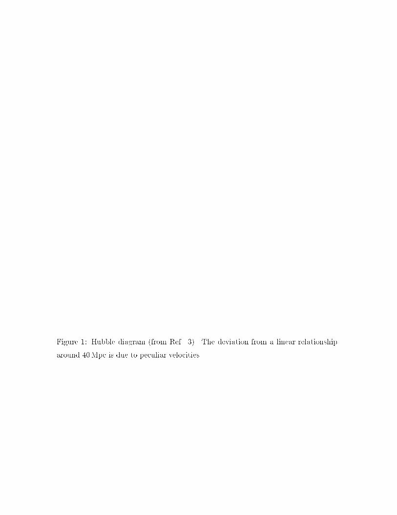
Figure 1: Hubble diagram (from Ref. 3). The deviation from a linear relationship
around 40Mpc is due to peculiar velocities.

seen out to redshifts of almost �ve (the current record holder is a quasar
with redshift 4.9). Thus, we can probe the universe with visible light to
within a few billion years of the Big Bang.
1.1.2 The Cosmic Background Radiation
The spectrum of the cosmic background radiation (CBR) is consistent
with that of a black body at temperature 2.73 K over more than three
decades in wavelength (� � 0:03 cm�100 cm); see Fig. 2. The most accu-
rate measurement of the temperature and spectrum is that by the FIRAS
instrument on the COBE satellite which determined its temperature to
be 2:726 � 0:005K (Ref. 7). It is di�cult to come up with a process
other than an early hot and dense phase in the history of the universe
that would lead to such a precise black body.8 According to the standard
cosmology, the surface of last scattering for the CBR is the universe at
a redshift of about 1100 and an age of about 180; 000 (0h2)�1=2 yrs. It
is possible that the universe became ionized again after this epoch, or
due to energy injection, never recombined; in this case, the last-scattering
surface is even \closer," zLSS ' 10[Bh=p0]
�2=3.
The temperature of the CBR is very uniform across the sky, to bet-
ter than a part in 104 on angular scales from arcminutes to 90 degrees;
see Fig. 3. Three forms of temperature anisotropy|two spatial and one
temporal|have now been detected: (1) a dipole anisotropy of about a
part in 103, generally believed to be due to the motion of a galaxy rela-
tive to the cosmic rest frame, at a speed of about 620 km sec�1 (Ref. 9);
(2) a yearly modulation in the temperature in a given direction on the
sky of about a part in 104, due to our orbital motion around the sun at
30 km sec�1, see Fig. 4 (Ref. 10); and (3) the temperature anisotropies
detected by the Di�erential Microwave Radiometer (DMR) on the Cos-
mic Background Explorer (COBE) satellite11 and more than ten other
experiments.12

Figure 2: (a) CBR spectrum as measured by the FIRAS on COBE. (b) Summary of
other CBR temperature measurements. (Figure courtesy of G. Smoot.)
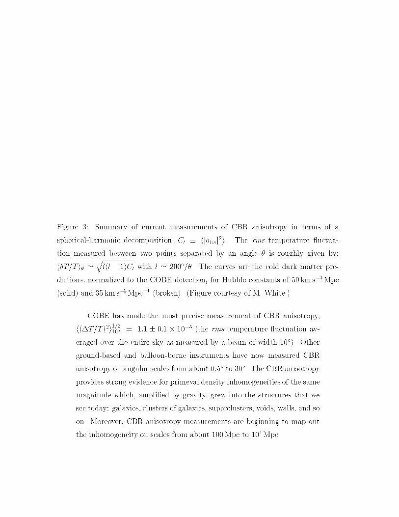
Figure 3: Summary of current measurements of CBR anisotropy in terms of a
spherical-harmonic decomposition, Cl � hjalmj2i. The rms temperature uctua-
tion measured between two points separated by an angle � is roughly given by:
(�T=T )� 'ql(l + 1)Cl with l ' 200�=�. The curves are the cold dark matter pre-
dictions, normalized to the COBE detection, for Hubble constants of 50 km s�1Mpc
(solid) and 35 km s�1Mpc�1 (broken). (Figure courtesy of M. White.)
COBE has made the most precise measurement of CBR anisotropy,
h(�T=T )2i1=210� = 1:1 � 0:1� 10�5 (the rms temperature uctuation av-
eraged over the entire sky as measured by a beam of width 10�). Other
ground-based and balloon-borne instruments have now measured CBR
anisotropy on angular scales from about 0:5� to 30�. The CBR anisotropy
provides strong evidence for primeval density inhomogeneities of the same
magnitude which, ampli�ed by gravity, grew into the structures that we
see today: galaxies, clusters of galaxies, superclusters, voids, walls, and so
on. Moreover, CBR anisotropy measurements are beginning to map out
the inhomogeneity on scales from about 100Mpc to 104Mpc.

Figure 4: Yearly modulation of the CBR temperature|the Earth really orbits the
Sun(!) (from Ref. 10).

1.1.3 Primordial Nucleosynthesis
Last, but certainly not least, there is the abundance of the light ele-
ments. According to the standard cosmology, when the age of the uni-
verse was measured in seconds, the temperatures were of order MeV, and
the conditions were right for nuclear reactions which ultimately led to
the synthesis of signi�cant amounts of D, 3He, 4He, and 7Li. The yields
of primordial nucleosynthesis depend upon the baryon density, quanti�ed
as the baryon-to-photon ratio �, and the number of very light (<� MeV)
particle species, often quanti�ed as the equivalent number of light neu-
trino species, N� . The predictions for the primordial abundances of all
four light elements agree with their measured abundances provided that
2:5� 10�10 <� � <� 6� 10�10 and N�<� 3:9; see Fig. 5 (Refs. 13-16).
Accepting the success of the standard model of nucleosynthesis, our
precise knowledge of the present temperature of the universe allows us
to convert � to a mass density and, by dividing by the critical density
�crit ' 1:88 h2�10�29 g cm�3, to the fraction of critical density contributed
by ordinary matter:
0:009 <� Bh2 <� 0:022; ) 0:01 <� B
<� 0:15; (1)
this is the most accurate determination of the baryon density. Note, the
uncertainty in the value of the Hubble constant leads to most of the un-
certainty in B .
The nucleosynthesis bound to N� , and more generally to the number
of light degrees of freedom in thermal equilibrium at the epoch of nu-
cleosynthesis, is consistent with precision measurements of the properties
of the Z0 boson, which give N� = 3:0 � 0:02; further, the cosmologi-
cal bound predates these accelerator measurements! The nucleosynthesis
bound provides a stringent limit to the existence of new, light particles
(even beyond neutrinos), and even provides a bound to the mass of the
tau neutrino, excluding a long-lived tau-neutrino of mass between 0:5MeV

Figure 5: Predicted light-element abundances including 2� theoretical uncertainties
(from Ref. 14). The inferred primordial abundances and concordance regions are
indicated.

and 30MeV.17,18 Primordial nucleosynthesis provides a beautiful illustra-
tion of the powers of the heavenly laboratory, though it is outside the focus
of these lectures.
The remarkable success of primordial nucleosynthesis gives us con�-
dence that the standard cosmology provides an accurate accounting of the
universe at least as early as 0:01 sec after the Bang, when the temperature
was about 10MeV.
1.1.4 Et Cetera|and the Age Crisis?
There are additional lines of reasoning and evidence that support the
standard cosmology.8 I mention two: the age of the universe and structure
formation. I will discuss the basics of structure formation a bit later;
for now, it su�ces to say that the standard cosmology provides a basic
framework for understanding the formation of structure|ampli�cation of
small primeval density inhomogeneities through gravitational instability.
Here, I focus on the age of the universe.
The expansion age of the universe|time back to zero size|depends
upon the present expansion rate, energy content, and equation of state:
texp = f(�; p)H�10 ' 9:8h�1f(�; p)Gyr. For a matter-dominated universe,
f is between 1 and 2/3 (for 0 between 0 and 1), so that the expansion
age is somewhere between 7Gyr and 20Gyr. There are other independent
measures of the age of the universe, e.g., based upon long-lived radioiso-
topes, the oldest stars, and the cooling of white dwarfs. These \ages,"
ranging from 13 to 18 Gyr, span the same interval(!).19 This wasn't al-
ways the case; as late as the early 1950s, it was believed that the Hubble
constant was 500 km sec�1Mpc�1, implying an expansion age of at most
2Gyr|less than the age of the Earth. This discrepancy was an important
motivation for the steady-state cosmology.
While there is general agreement between the expansion age and other
determinations of the age of the universe, some cosmologists are worried
that cosmology is on the verge of another age crisis.5 Let me explain.
While Sandage and a few others continue to obtain values for the Hubble
constant around 50 km s�1Mpc�1 (Ref. 2), a variety of di�erent techniques
seem to be converging on a value around 80� 10 km s�1Mpc�1 (Ref. 5).
If H0 = 80 km s�1Mpc�1, then texp = 12f(�; p)Gyr, and for 0 = 1,
texp = 8 Gyr, which is clearly inconsistent with other measures of the age.
If H0 = 80 km s�1 Mpc�1, one is almost forced to consider the radical
alternative of a cosmological constant. For example, even with 0 = 0:2,
f ' 0:85, corresponding to texp ' 10Gyr; on the other hand, for a at
universe with � = 0:7, f ' 1 and the expansion age texp ' 12 Gyr. As
I shall discuss later, structure formation provides another motivation for
a cosmological constant. As mentioned earlier, the detection of Cepheid
variables in Virgo6 is a giant step toward an accurate determination of
H0, and it seems likely that the issue may be settled soon.
1.2 Basics of the Big Bang Model
The standard cosmology is based upon the maximally, spatially symmetric
Robertson-Walker line element
ds2 = dt2 �R(t)2"
dr2
1� kr2+ r2(d�2 + sin2 � d�2)
#; (2)
where R(t) is the cosmic-scale factor, Rcurv � R(t)jkj�1=2 is the curvatureradius, and k=jkj = �1; 0; 1 is the curvature signature. All three models
are without boundary|the positively curved model is �nite and \curves"
back on itself; the negatively curved and at models are in�nite in extent
(though �nite versions of both can be constructed by imposing a periodic
structure|identifying all points in space with a fundamental cube). The
Robertson-Walker metric embodies the observed isotropy and homogene-
ity of the universe. It is interesting to note that this form of the line
element was originally introduced for the sake of mathematical simplicity;
we now know that it is well-justi�ed at early times or today on large scales
(� 10Mpc), at least within our Hubble volume.
The coordinates, r, �, and �, are referred to as comoving coordinates.
A particle at rest in these coordinates remains at rest, i.e., constant r, �,
and �. A freely moving particle eventually comes to rest at these coordi-
nates, as its momentum is redshifted by the expansion, p / R�1. Motion
with respect to the comoving coordinates (or cosmic rest frame) is re-
ferred to as peculiar velocity; unless \supported" by the inhomogeneous
distribution of matter, peculiar velocities decay away as R�1. Thus the
measurement of peculiar velocities, which is not easy as it requires inde-
pendent measures of both the distance and velocity of an object, can be
used to probe the distribution of mass in the universe.
Physical separations (i.e., measured by meter sticks) between freely
moving particles scale as R(t), or said another way, the physical separation
between two points, are simply R(t) times the coordinate separation. The
momenta of freely propagating particles decrease, or \redshift," as R(t)�1,
and thus the wavelength of a photon stretches as R(t), which is the origin
of the cosmological redshift. The redshift su�ered by a photon emitted
from a distant galaxy is 1 + z = R0=R(t); that is, a galaxy whose light
is redshifted by 1 + z emitted that light when the universe was a factor
of (1 + z)�1 smaller. Thus, when the light from the most distant quasar
yet seen (z = 4:9) was emitted, the universe was a factor of almost six
smaller; when CBR photons last scattered, the universe was about 1100
times smaller.
1.2.1 Friedmann Equation and the First Law
The evolution of the cosmic-scale factor is governed by the Friedmann
equation
H2 � _R
R
!2=
8�G�tot3
� k
R2; (3)

where �tot is the total energy density of the universe, matter, radiation,
vacuum energy, and so on. A cosmological constant is often written as an
additional term (= �=3) on the rhs; I will choose to treat it as a constant
energy density (\vacuum-energy density"), where �vac = �=8�G. (My
convention in this regard is not universal.) The evolution of the energy
density of the universe is governed by
d(�R3) = �pdR3; (4)
which is the First Law of Thermodynamics for a uid in the expanding
universe. (In the case that the stress energy of the universe is comprised
of several, noninteracting components, this relation applies to each sepa-
rately; e.g., to the matter and radiation separately today.) For p = �=3,
ultrarelativistic matter, � / R�4; for p = 0, very nonrelativistic matter,
� / R�3; and for p = ��, vacuum energy, � = const. If the rhs of the
Friedmann equation is dominated by a uid with equation of state p = �,
it follows that � / R�3(1+ ) and R / t2=3(1+ ).
We can use the Friedmann equation to relate the curvature of the
universe to the energy density and expansion rate:
k=R2
H2= � 1; =
�tot
�crit; (5)
and the critical density today �crit = 3H2=8�G = 1:88h2 g cm�3 ' 1:05�104 eV cm�3. There is a one-to-one correspondence between and the
spatial curvature of the universe: positively curved, 0 > 1; negatively
curved, 0 < 1; and at (0 = 1). Further, the \fate of the universe" is
determined by the curvature. Model universes with k � 0 expand forever,
while those with k > 0 necessarily recollapse. The curvature radius of the
universe is related to the Hubble radius and by
Rcurv =H�1
j� 1j1=2 : (6)
In physical terms, the curvature radius sets the scale for the size of spatial
separations where the e�ects of curved space become \pronounced." And

in the case of the positively curved model, it is just the radius of the
three-sphere.
The energy content of the universe consists of matter and radiation (to-
day, photons and neutrinos). Since the photon temperature is accurately
known, T0 = 2:73 � 0:01K, the fraction of critical density contributed
by radiation is also accurately known: radh2 = 4:18� 10�5. The matter
content is another matter.
1.2.2 A Short Diversion Concerning the Present Mass Density
The matter density today, i.e., the value of 0, is not nearly so well-
known.20 Stars contribute much less than 1% of critical density; based
upon nucleosynthesis, we can infer that baryons contribute between 1%
and 15% of critical density. The dynamics of various systems allow as-
tronomers to infer their gravitational mass. With their telescopes, they
measure the amount of light and form a mass-to-light ratio. Multiplying
this by the measured luminosity density of the universe gives a determina-
tion of the mass density. (The criticalmass-to-light ratio is 1200hM�=L�.)The motions of stars and gas clouds in spiral galaxies indicate that
most of the mass of spiral galaxies exists in the form of dark (i.e., no
detectable radiation), extended halos, whose full extent is still not known.
Many cite the at rotation curves of spiral galaxies, which indicate that
the halo density decreases as r�2, as the best evidence that most of the
matter in the universe is dark. Taking the mass-to-light ratio inferred for
spiral galaxies to be typical of the universe as a whole and remembering
that the full extent of the dark matter halos is not known, one infers
halo >� 0:03� 0:1 (Ref. 21).
The masses of clusters of galaxies have been determined by applying
the virial theorem to the motions of member galaxies or to the hot gas
that �lls the intracluster medium, and by analyzing (weak) gravitational
lensing of very distant galaxies by clusters. These mass estimates also
indicate the presence of large amounts of dark matter; when more than one
method is applied to the same cluster, the mass estimates are consistent.
Taking cluster mass-to-light ratios to be typical of the universe as a whole,
in spite of the fact that only about one in ten galaxies resides in a cluster,
one infers cluster � 0:2� 0:4.
Another interesting fact has been learned from x-ray observations of
clusters|the ratio of baryons in the hot intracluster gas to the total cluster
mass, Mgas=Mtot ' (0:04 � 0:08)h�3=2 (Ref. 22). Since the gas mass is
much greater than the mass in the visible galaxies, this ratio provides an
estimate of the cluster baryon fraction, provided that most of the baryons
reside in the hot gas or in galaxies, and suggests that the bulk of matter
in clusters is in a form other than baryons!
Not one of these methods is wholly satisfactory. Rotation curves of
spiral galaxies are still \ at" at the last measured points, indicating that
the mass is still increasing; likewise, cluster virial mass estimates are in-
sensitive to material that lies beyond the region occupied by the visible
galaxies|and moreover, only about one galaxy in ten resides in a cluster.
What one would like is a measurement of the mass of a very big sample
of the universe, say a cube of 100h�1Mpc on a side, which contains tens
of thousands of galaxies.
Over the past �ve years or so, progress has been made toward such
a measurement. It involves the peculiar motion of our own galaxy, at a
speed of about 620 km sec�1 in the general direction of Hydra-Centaurus.
This motion is due to the lumpy distribution of matter in our vicinity. By
using gravitational-perturbation theory (actually, not much more than
Newtonian physics) and the distribution of galaxies in our vicinity (as
determined by the IRAS catalogue of infrared selected galaxies), one can
infer the average mass density in a very large volume and thereby 0.
The basic physics behind the method is simple: the net gravitational
pull on our galaxy depends both upon how inhomogeneous the distribution
of galaxies is and how much mass is associated with each galaxy; by
measuring the distribution of galaxies and our peculiar velocity, one can
infer the \mass per galaxy" and 0.
The value that has been inferred is big(!)|close to unity|and provides
a very strong case that 0 is at least 0.3 (Ref. 23). Moreover, the measured
peculiar velocities of other galaxies in this volume, more than a thousand,
have been used in a similar manner and indicate a similarly large value
for 0 (Ref. 24). While this technique is very powerful, it does have its
drawbacks. One has to make simple assumptions about how accurately
mass is traced by light (the observed galaxies); one has to worry whether
or not a signi�cant portion of our galaxy's velocity is due to galaxies
outside the IRAS sample|if so, this would lead to an overestimate of 0;
and so on. This technique is not only very promising|but provides the
\correct" answer (in my opinion!).
The so-called classical kinematic tests|Hubble diagram, angle redshift
relation, galaxy count-redshift relation|can, in principle, provide a de-
termination of 0 by determining the deceleration parameter q0 (Ref. 25).
However, all these methods require standard candles, rulers, or galaxies,
and for this reason, have proved inconclusive. However, that has not dis-
couraged anyone. There are a number of e�orts to determine q0 using the
galaxy number-count test,26 and two groups are trying to measure q0 by
constructing a Hubble diagram based upon Type Ia supernovae (out to
redshifts of 0.5 or more).
To summarize this aside on the mass density of the universe:
1. Most of the matter is dark.
2. Baryons provide between about 1% and 15% of the mass density
(allowing 0:4 < h < 1; taking h > 0:6, the upper limit decreases to
6%).

3. There is a strong case that 0>� 0:3 (peculiar velocities), a convincing
case that 0>� 0:2 (cluster masses), and an airtight case that 0
>�0:1 ( at rotation curves of spirals).
4. Most of the baryons are dark (not in stars). In clusters, the bulk of
the baryons are in hot gas.
5. The evidence for nonbaryonic dark matter continues to mount; e.g.,
the gap between B and 0 and the cluster baryon fraction.
The current prejudice|and certainly that of this author|is a at uni-
verse (0 = 1) with nonbaryonic dark matter, X � 1� B. However,
I shall continue to display the 0 dependence of important quantities.
1.2.3 The Early, Radiation-Dominated Universe
In any case, at present, matter outweighs radiation by a wide margin.
However, since the energy density in matter decreases as R�3, and that
in radiation as R�4 (the extra factor due to the redshifting of the en-
ergy of relativistic particles), at early times the universe was radiation
dominated|indeed the calculations of primordial nucleosynthesis provide
excellent evidence for this. Denoting the epoch of matter-radiation equal-
ity by subscript \EQ" and using T0 = 2:73K, it follows that
REQ = 4:18� 10�5 (0h2)�1; TEQ = 5:62(0h
2) eV; (7)
tEQ = 4:17� 1010(0h2)�2 sec: (8)
At early times, the expansion rate and age of the universe were determined
by the temperature of the universe and the number of relativistic degrees
of freedom:
�rad = g�(T )�2T 4
30; H ' 1:67g1=2� T 2=mP l; (9)
) R / t1=2; t ' 2:42� 10�6g�1=2� (T=GeV)�2 sec; (10)

Figure 6: The total e�ective number of relativistic degrees of freedom g�(T ) in the
standard model of particle physics as a function of temperature.
where g�(T ) counts the number of ultrarelativistic degrees of freedom
(� the sum of the internal degrees of freedom of particle species much
less massive than the temperature) and mP l � G�1=2 = 1:22�1019GeV is
the Planck mass. For example, at the epoch of nucleosynthesis, g� = 10:75
assuming three, light (� MeV) neutrino species; taking into account all
the species in the Standard Model, g� = 106:75 at temperatures much
greater than 300GeV; see Fig. 6.
A quantity of importance related to g� is the entropy density in rela-
tivistic particles,
s =�+ p
T=
2�2
45g�T
3;
and the entropy per comoving volume,
S / R3s / g�R3T 3:

By a wide margin, most of the entropy in the universe exists in the radi-
ation bath. The entropy density is proportional to the number density of
relativistic particles. At present, the relativistic particle species are the
photons and neutrinos, and the entropy density is a factor of 7.04 times
the photon-number density: n = 413 cm�3 and s = 2905 cm�3.
In thermal equilibrium|which provides a good description of most of
the history of the universe|the entropy per comoving volume S remains
constant. This fact is very useful. First, it implies that the temperature
and scale factor are related by
T / g�1=3� R�1; (11)
which for g� =const leads to the familiar T / R�1.
Second, it provides a way of quantifying the net baryon number (or
any other particle number) per comoving volume:
NB � R3nB =nB
s' (4� 7)� 10�11: (12)
The baryon number of the universe tells us two things: (1) the entropy
per particle in the universe is extremely high, about 1010 or so compared
to about 10�2 in the sun and a few in the core of a newly formed neutron
star. (2) The asymmetry between matter and antimatter is very small,
about 10�10, since at early times quarks and antiquarks were roughly as
abundant as photons. One of the great successes of particle cosmology is
baryogenesis, the idea that B, C, and CP violating interactions occurring
out-of-equilibrium early on allow the universe to develop a net baryon
number of this magnitude.27
Finally, the constancy of the entropy per comoving volume allows us
to characterize the size of comoving volume corresponding to our present
Hubble volume in a very physical way. By the entropy it contains,
SU =4�
3H�30 s ' 1090: (13)

1.2.4 The Earliest History
The standard cosmology is tested back to times as early as about 0.01 sec;
it is only natural to ask how far back one can sensibly extrapolate. Since
the fundamental particles of nature are point-like quarks and leptons
whose interactions are perturbatively weak at energies much greater than
1GeV, one can imagine extrapolating as far back as the epoch where
general relativity becomes suspect, i.e., where quantum gravitational ef-
fects are likely to be important: the Planck epoch, t � 10�43 sec, and
T � 1019GeV. Of course, at present, our �rm understanding of the ele-
mentary particles and their interactions only extends to energies of the or-
der of 100GeV, which corresponds to a time of the order of 10�11 sec or so.
We can be relatively certain that at a temperature of 100MeV�200MeV
(t � 10�5 sec), there was a transition (likely a second-order phase tran-
sition) from quark/gluon plasma to very hot hadronic matter, and that
some kind of phase transition associated with the symmetry breakdown
of the electroweak theory took place at a temperature of the order of
300GeV (t � 10�11 sec).
It is interesting to look at the progress that has taken place since
Weinberg's classic text on cosmology was published in 1972 (Ref. 28);
at that time, many believed that the universe had a limiting tempera-
ture of the order of several hundred MeV, due to the exponentially rising
number of particle states, and that one could not speculate about earlier
times. Today, based upon our present knowledge of physics and powerful
mathematical tools (e.g., gauge theories, grand uni�ed theories, and su-
perstring theory), we are able to make quantitative speculations back to
the Planck epoch|and even earlier. Of course, these speculations could
be totally wrong, based upon a false sense of con�dence (arrogance?). As I
shall discuss, in ation is one of these well-de�ned|and well-motivated|
speculations about the history of the universe well after the Planck epoch,
but well before primordial nucleosynthesis.
1.2.5 The Matter and Curvature-Dominated Epochs
After the equivalence epoch, the matter density exceeds that of radiation.
During the matter-dominated epoch, the scale factor grows as t2=3 and
the age of the universe is related to redshift by
t = 2:06� 1017(0h2)�1=2(1 + z)�3=2 sec: (14)
If 0 < 1, the matter-dominated epoch is followed by a \curvature-
dominated" epoch where the rhs of the Friedmann equation is dominated
by the jkj=R2 term. When the universe is curvature dominated, it is said
to expand freely, no longer decelerating since the gravitational e�ect of
matter has become negligible: �R � 0 and R / t. The epoch of curvature
dominance begins when the matter and curvature terms are equal:
RCD =0
1�0
�! 0; zCD = �10 � 2 �! �1
0 ; (15)
where the limits shown are for 0 ! 0. By way of comparison, in a
at universe with a cosmological constant, the universe becomes \vacuum
dominated" when R = Rvac:
Rvac =�
0
1� 0
�1=3�!
1=30 ; zvac =
�1�0
0
�1=3� 1 �!
�1=30 :
(16)
For a given value of 0, the transition occurs much more recently, which
has important implications for structure formation since small density
perturbations only grow during the matter-dominated era.
1.2.6 One Last Thing: Horizons
In spite of the fact that the universe was vanishingly small at early
times, the rapid expansion precluded causal contact from being established
throughout. Photons travel on null paths characterized by dr = dt=R(t);
the physical distance that a photon could have traveled since the Bang

until time t, the distance to the horizon, is
dH(t) = R(t)Z t
0
dt0
R(t0)
= t=(1� n) = nH�1=(1� n) for R(t) / tn; n < 1: (17)
Note, in the standard cosmology the distance to the horizon is �nite, and
up to numerical factors, equal to the age of the universe or the Hubble
radius, H�1. For this reason, I will use \horizon" and \Hubble radius"
interchangeably.�An important quantity is the entropy within a horizon volume: SHOR �
H�3T 3 during the radiation-dominated epoch H � T 2=mP l, so that
SHOR ��mP l
T
�3; (18)
from this, we conclude that at early times the comoving volume that en-
compasses all that we can see today (characterized by an entropy of 1090)
was comprised of a very large number of causally disconnected regions.
1.3 Two Challenges: Dark Matter and Structure
Formation
These two challenges are not unrelated: a detailed understanding of the
formation of structure in the universe necessarily requires knowledge of
the quantity and composition of matter in the universe.
We have every indication that the universe at early times, say t �300; 000 yrs, was very homogeneous; however, today inhomogeneity (or
structure) is ubiquitous: stars (��=� � 1030), galaxies (��=� � 105), clus-
ters of galaxies (��=� � 10� 103), superclusters, or \clusters of clusters"
(��=� � 1), voids (��=� � �1), great walls, and so on.
�In in ationary models, the horizon and Hubble radius are not roughly equal as the horizon distance
grows exponentially relative to the Hubble radius; in fact, at the end of in ation they di�er by eN ,
where N is the number of e-folds of in ation. However, I will slip and use \horizon" and \Hubble
radius" interchangeably, though I will always mean Hubble radius.

For some 25 years, the standard cosmology has provided a general
framework for understanding this. Once the universe becomes matter
dominated (around 1000 yrs. after the Bang), primeval density inho-
mogeneities (��=� � 10�5) are ampli�ed by gravity and grow into the
structure we see today.29 The fact that a uid of self-gravitating particles
is unstable to the growth of small inhomogeneities was �rst pointed out
by Jeans and is known as the Jeans instability. The existence of these in-
homogeneities was con�rmed in spectacular fashion by the COBE DMR
discovery of CBR anisotropy.
At last, the basic picture has been put on �rm ground (whew!). Now
the challenge is to �ll in the details|origin of the density perturbations,
precise evolution of the structure, and so on. As I shall emphasize, such
an understanding may well be within reach and o�ers a window on the
early universe.
1.3.1 The General Picture: Gravitational Instability
Let us begin by expanding the perturbation to the matter density in plane
waves��M (x; t)
�M=
1
(2�)3
Zd3k �k(t)e
�ik�x; (19)
where � = 2�=k is the comoving wavelength of the perturbation and
�phys = R� is the physical wavelength. The comoving wavelengths of
perturbations corresponding to bright galaxies, clusters, and the present
horizon scale are respectively: about 1Mpc, 10Mpc, and 3000h�1Mpc,
where 1Mpc ' 3:09� 1024 cm ' 1:56� 1038GeV�1.
The growth of small matter inhomogeneities of wavelengths smaller
than the Hubble scale (�phys <� H�1) is governed by a Newtonian equation:
��k + 2H _�k + v2sk2�k=R
2 = 4�G�M�k; (20)
where v2s = dp=d�M is the square of the sound speed. Competition
between the pressure term and the gravity term on the rhs determine

whether or not pressure can counteract gravity. Perturbations with wave-
numbers larger than the Jeans wavenumbers, k2J = 4�GR2�M=v2s , are
Jeans stable and just oscillate; perturbations with smaller wavenumbers
are Jeans unstable and can grow. For cold dark matter, vs ' 0 and all
scales are Jeans unstable; even for baryonic matter, after decoupling, kJ
corresponds to a baryon mass of only about 105M�. All the scales of
interest here are Jeans unstable, and we will ignore the pressure term.
Let us discuss solutions to this equation under di�erent circumstances.
First, consider the Jeans problem, evolution of perturbations in a static
uid, i.e., H = 0. In this case, Jeans unstable perturbations grow ex-
ponentially, �k / exp(t=�) where � = 1=p4G��M . Next, consider the
growth of Jeans unstable perturbations in a matter-dominated universe,
i.e., H2 = 8�G�M=3 and R / t2=3. Because the expansion tends to \pull
particles away from one another," the growth is only power law, �k / t2=3;
i.e., at the same rate as the scale factor. Finally, consider a radiation-
or curvature-dominated universe, i.e., 8�G�rad=3 or jkj=R2 much greater
than 8�G�M=3. In this case, the expansion is so rapid that matter per-
turbations grow very slowly, as lnR in a radiation-dominated epoch, or
not at all; �k =const in the curvature-dominated epoch.
The growth of nonlinear perturbations is another matter; once a per-
turbation reaches an overdensity of order unity or larger, it \separates"
from the expansion|i.e., becomes its own self-gravitating system and
ceases to expand any further. In the process of virial relaxation, its size
decreases by a factor of two|density increases by a factor of eight; there-
after, its density contrast grows as R3 since the average matter density
is decreasing as R�3, though smaller scales could become Jeans unstable
and collapse further to form smaller objects of higher density, stars, etc.
From this, we learn that structure formation begins when the universe
becomes matter dominated and ends when it becomes curvature dom-
inated (at least the growth of linear perturbations). The total growth
available for linear perturbations is RCD=REQ ' 2:4�10420h
2; since non-
linear structures have evolved by the present epoch, we can infer that
primeval perturbations of the order (��M=�M)EQ � 4� 10�5 (0h)�2 are
required. Note that in a low-density universe, larger initial perturbations
are necessary as there is less time for growth (\the low 0 squeeze"). Fur-
ther, in a baryon-dominated universe, things are even more di�cult as
perturbations in the baryons cannot begin to grow until after decoupling
since matter is tightly coupled to the radiation. (In a at, low-0 model
with a cosmological constant, the growth of linear uctuations continues
almost until today since z� � �1=30 , and so the total growth factor is
about 2:4� 104(0h2). We will return to this model later.)
1.3.2 CBR Temperature Fluctuations
The existence of density inhomogeneities has another important conse-
quence: uctuations in the temperature of the CBR of a similar ampli-
tude.30 The temperature di�erence measured between two points sepa-
rated by a large angle (>� 1�) arises due to a very simple physical e�ect.yThe di�erence in the gravitational potential between the two points on
the last-scattering surface, which in turn is related to the density per-
turbation, determines the temperature anisotropy on the angular scale
subtended by that length scale,
�T
T
!�
= � ��
3
!�
� 1
2
��
�
!HOR;�
; (21)
where the scale � � 100h�1Mpc(�=deg) subtends an angle � on the last-
scattering surface. This is known as the Sachs-Wolfe e�ect.31
yLarge angles mean those larger than the angle subtended by the horizon-scale at decoupling,
� � H�1
DEC=H�1
0� z
�1=2
DEC� 1�.

The quantity (��=�)HOR;� is the amplitude with which a density per-
turbation crosses inside the horizon, i.e., when R� � H�1. Since the uc-
tuation in the gravitational potential �� � (R�=H�1)2(��=�), the horizon-
crossing amplitude is equal to the gravitational potential (or curvature)
uctuation. The horizon-crossing amplitude (��=�)HOR has several nice
features: (i) during the matter-dominated era, the potential uctuation
on a given scale remains constant, and thus the potential uctuations at
decoupling on scales that crossed inside the horizon after matter-radiation
equality, corresponding to angular scales <� 0:1�, are just given by their
horizon-crossing amplitude; (ii) because of its relationship to ��, it pro-
vides a dimensionless, geometrical measure of the size of the density per-
turbation on a given scale and its e�ect on the CBR; (iii) by specifying
perturbation amplitudes at horizon crossing, one can e�ectively avoid dis-
cussing the evolution of density perturbations on scales larger than the
horizon, where a Newtonian analysis does not su�ce and where gauge
subtleties (associated with general relativity) come into play; and �nally,
(iv) the density perturbations generated in in ationary models are char-
acterized by (��=�)HOR ' const.
On angular scales smaller than about 1�, two other physical e�ects lead
to CBR temperature uctuations: the motion of the last-scattering surface
(Doppler) and the intrinsic uctuations in the local photon temperature.
These uctuations are much more di�cult to compute and depend on
microphysics|the ionization history of the universe and the damping of
perturbations in the photon-baryon uid due to photon streaming. Not
only are the Sachs-Wolfe uctuations simpler to compute, but they accu-
rately mirror the primeval uctuations since at the epoch of decoupling,
microphysics is restricted to angular scales less than about a degree.
In sum, on large angular scales, the Sachs-Wolfe e�ect dominates; on
the scale of about 1�, the total CBR uctuation is about twice that due to
the Sachs-Wolfe e�ect; on smaller scales, the Doppler and intrinsic uc-

tuations dominate (see Fig. 3). CBR temperature uctuations on scales
smaller than about 0:1� are severely reduced by the smearing e�ect of the
�nite thickness of last-scattering surface. (For a beautiful exposition of
how CBR anisotropy arises, see Ref. 32).
Details aside, in the context of the gravitational instability scenario,
density perturbations of su�cient amplitude to explain the observed struc-
ture lead to temperature uctuations in the CBR of characteristic size,
�T
T� 10�5 (0h)
�2: (22)
To be sure, I have brushed over important details, but this equation con-
veys a great deal. First, the overall amplitude is set by the inverse of
the growth factor, which is just the ratio of the radiation energy den-
sity to matter density at present. Next, it explains why theoretical cos-
mologists were so relieved when the COBE DMR detected temperature
uctuations of this amplitude, and conversely, why one heard o�handed
remarks before the COBE DMR detection that the standard cosmology
was in trouble because the CBR temperature was too uniform to allow
for the observed structure to develop. Finally, it illustrates one of the
reasons why cosmologists who study structure formation have embraced
the at-universe model with such enthusiasm|if we accept the universe
that meets the eye, 0 � 0:1 and baryons only, then the simplest models
of structure formation predict temperature uctuations of the order of
10�3, far too large to be consistent with observation. Later, I will men-
tion Peebles' what-you-see-is-what-you-get model,33 also known as PIB
for primeval isocurvature baryon uctuation, which is still viable because
the spectrum of perturbations decreases rapidly with scale so that the
perturbations that give rise to CBR uctuations are small (which is no
mean feat). Historically, it was fortunate that one started with a low-
0, baryon-dominated universe. The theoretical predictions for the CBR
uctuations were su�ciently favorable that experimentalists were stirred
to try to measure them|and then, slowly, theorists lowered their predic-

tions. Had the theoretical expectations begun at 10�5, experimentalists
might have been too discouraged to even try!
1.3.3 An Initial Data Problem
With the COBE DMR detection in hand, we can praise the success of
the gravitational instability scenario; however, the details now remain to
be �lled in. The structure formation problem is now one of initial data,
namely:
1. The quantity and composition of matter in the universe, 0, B, and
other.
2. The spectrum of initial density perturbations: for the purist, (��=�)HOR,
or for the simulator, the Fourier amplitudes at the epoch of matter-
radiation equality.
In a statistical sense, these initial data provide the \blueprint" for the
formation of structure.
The initial data are the challenge and the opportunity. Although
the gravitational instability picture has been around since the discov-
ery of the CBR itself, the lack of speci�city in initial data has impeded
progress. With the advent of the study of the earliest history of the uni-
verse, a new door was opened. We now have several well motivated early-
universe blueprints: in ation-produced density perturbations and non-
baryonic dark matter; cosmic-string produced perturbations and nonbary-
onic dark matter;34 texture-produced density perturbations and nonbary-
onic dark matter;35 and one \conventional model," a baryon-dominated
universe with isocurvature uctuationsz.33 Structure formation provides
the opportunity to probe the earliest history of the universe. I will focus
zIsocurvature baryon-number uctuations correspond at early times to uctuations in the local
baryon number but not the energy density. At late times, when the universe is matter-dominated,
they become uctuations in the mass density of a comparable amplitude.

on the cold dark matter \family of models," which are motivated by in-
ation. Already, the ood of data has all but eliminated the conventional
model; the texture and cosmic-string models face severe problems with
CBR anisotropy|and who knows, even the cold dark matter models may
be eliminated.
2 In ationary Theory
2.1 Generalities
As successful as the Big Bang cosmology is, it su�ers from a dilemma
involving initial data. Extrapolating back, one �nds that the universe
apparently began from a very special state: a slightly inhomogeneous and
very at Robertson-Walker spacetime. Collins and Hawking showed that
the set of initial data that evolve to a spacetime that is as smooth and
at as ours is today of measure zero.36 (In the context of simple grand
uni�ed theories, the hot Big Bang su�ers from another serious problem:
the extreme overproduction of superheavy magnetic monopoles; in fact,
it was an attempt to solve the monopole problem which led Guth to
in ation.)
The cosmological appeal of in ation is its ability to lessen the depen-
dence of the present state of the universe upon the initial state. Two
elements are essential to doing this: (1) accelerated (\superluminal") ex-
pansion and the concomitant tremendous growth of the scale factor, and
(2) massive entropy production.38 Together, these two features allow a
small, smooth subhorizon-sized patch of the early universe to grow to a
large enough size and contain enough heat (entropy in excess of 1088) to
easily encompass our present Hubble volume. Provided that the region
was originally small compared to the curvature radius of the universe, it
would appear at then and today (just as any small portion of the surface
of a sphere appears at).

While there is presently no standard model of in ation|just as there
is no standard model for physics at these energies (typically 1015GeV or
so)|viable models have much in common. They are based upon well-
posed, albeit highly speculative, microphysics involving the classical evo-
lution of a scalar �eld. The superluminal expansion is driven by the
potential energy (\vacuum energy") that arises when the scalar �eld is
displaced from its potential-energy minimum, which results in nearly ex-
ponential expansion. Provided the potential is at, during the time it
takes for the �eld to roll to the minimum of its potential, the universe
undergoes many e-foldings of expansion (more than around 60 or so are
required to realize the bene�cial features of in ation). As the scalar �eld
nears the minimum, the vacuum energy has been converted to coherent
oscillations of the scalar �eld, which correspond to nonrelativistic scalar-
�eld particles. The eventual decay of these particles into lighter particles
and their thermalization results in the \reheating" of the universe and
accounts for all the heat in the universe today (the entropy production
event).
Superluminal expansion and the tremendous growth of the scale fac-
tor (by a factor greater than that since the end of in ation) allow quan-
tum uctuations on very small scales (<� 10�23 cm) to be stretched to
astrophysical scales (>� 1025 cm). Quantum uctuations in the scalar �eld
responsible for in ation ultimately lead to an almost scale-invariant spec-
trum of density perturbations,39 and quantum uctuations in the metric
itself lead to an almost scale-invariant spectrum of gravity-waves.40 Scale
invariance for density perturbations means scale-independent uctuations
in the gravitational potential (equivalently, density perturbations of di�er-
ent wavelengths cross the horizon with the same amplitude); scale invari-
ance for gravity waves means that gravity waves of all wavelengths cross
the horizon with the same amplitude. Because of subsequent evolution,
neither the scalar nor the tensor perturbations are scale invariant today.

2.2 Metaphysical Implications
In ation alleviates the \specialness" problem greatly, but does not elim-
inate all dependence upon the initial state.41 All open FRW models will
in ate and become at; however, many closed FRW models will recollapse
before they can in ate. If one imagines the most general initial spacetime
as being comprised of negatively and positively curved FRW (or Bianchi)
models that are stitched together, the failure of the positively curved re-
gions to in ate is of little consequence. Because of exponential expansion
during in ation, the negatively curved regions will occupy most of the
space today. Nor does in ation solve the smoothness problem forever; it
just postpones the problem into the exponentially distant future. We will
be able to see outside our smooth in ationary patch, and will start to
deviate signi�cantly from unity at a time t � t0 exp[3(N �Nmin)], where
N is the actual number of e-foldings of in ation and Nmin � 60 is the
minimum required to solve the horizon/ atness problems.
Linde has emphasized that in ation has changed our view of the uni-
verse in a very fundamental way.42 While cosmologists have long used the
Copernican principle to argue that the universe must be smooth because
of the smoothness of our Hubble volume, in the postin ation view, our
Hubble volume is smooth because it is a small part of a region that under-
went in ation. On the largest scales, the structure of the universe is likely
to be very rich. Di�erent regions may have undergone di�erent amounts
of in ation, may have di�erent laws of physics because they evolved into
di�erent vacuum states (of equivalent energy), and may even have dif-
ferent numbers of spatial dimensions. Since it is likely that most of the
volume of the universe is still undergoing in ation and that in ationary
patches are being constantly produced (eternal in ation), the age of the
universe is a meaningless concept and our expansion age merely measures
the time back to the end of our in ationary event!
2.3 Models
In Guth's seminal paper,43 he introduced the idea of in ation, sung its
praises, and showed that the model that he based the idea upon did not
work! Thanks to very important contributions by Linde44 and Albrecht
and Steinhardt,45 that was quickly remedied, and today there are many
viable models of in ation. That, of course, is both good news and bad
news; it means that there is no standard model of in ation. Again, the
absence of a standard model of in ation should be viewed in the light of
our general ignorance about fundamental physics at these energies.
Many di�erent approaches have been taken in constructing particle-
physics models for in ation. Some have focused on very simple scalar
potentials, e.g., V (�) = ��4 or = m2�2=2, without regard to connect-
ing the model to any underlying theory.46,47 Others have proposed more
complicatedmodels that attempt to make contact with speculations about
physics at very high energies, e.g., grand uni�cation,48 supersymmetry,49{51
preonic physics,52 or supergravity.53 Several authors have attempted to
link in ation with superstring theory54 or \generic predictions" of su-
perstring theory such as pseudo-Nambu-Goldstone boson �elds.55 While
the scale of the vacuum energy that drives in ation is typically of order
(1015GeV)4, a model of in ation at the electroweak scale, vacuum energy
� (1TeV)4, has been proposed.56 There are also models in which there
are multiple epochs of in ation.57
In all of the models above, gravity is described by general relativity.
A qualitatively di�erent approach is to consider in ation in the context
of alternative theories of gravity. (After all, in ation probably involves
physics at energy scales not too di�erent from the Planck scale, and the
e�ective theory of gravity at these energies could well be very di�erent
from general relativity; in fact, there are some indications from super-
string theory that gravity in these circumstances might be described by
a Brans-Dicke like theory.) Perhaps the most successful of these models

is �rst-order in ation.58,59 First-order in ation returns to Guth's original
idea of a strongly �rst-order phase transition; in the context of general
relativity, Guth's model failed because the phase transition, if in ation-
ary, never completed. In theories where the e�ective strength of gravity
evolves, like Brans-Dicke theory, the weakening of gravity during in ation
allows the transition to complete. In other models based upon nonstan-
dard gravitation theory, the scalar �eld responsible for in ation is itself
related to the size of additional spatial dimensions, and in ation then
also explains why our three spatial dimensions are so big, while the other
spatial dimensions are so small.
All models of in ation have one feature in common|the scalar �eld
responsible for in ation has a very at potential-energy curve and is very
weakly coupled. This typically leads to a very small dimensionless num-
ber, usually a dimensionless coupling of the order of 10�14. Such a small
number, like other small numbers in physics (e.g., the ratio of the weak
to Planck scales � 10�17 or the ratio of the mass of the electron to the
W=Z boson masses � 10�5), runs counter to one's belief that a truly
fundamental theory should have no tiny parameters, and cries out for
an explanation. At the very least, this small number must be stabilized
against quantum corrections|which it is in all of the previously men-
tioned models.x In some models, the small number in the in ationary
potential is related to other small numbers in particle physics|for exam-
ple, the ratio of the electron mass to the weak scale or the ratio of the
uni�cation scale to the Planck scale. Explaining the origin of the small
number that seems to be associated with in ation is both a challenge and
an opportunity.
xIt is sometimes stated that in ation is unnatural because of the small coupling of the scalar �eld
responsible for in ation; while the small coupling certainly begs explanation, these in ationary
models are not unnatural in the rigorous technical sense as the small number is stable against
quantum uctuations.

Because of the growing base of observations that bear on in ation,
another approach to model building is emerging|the use of observations
to constrain the underlying in ationary potential. I will return to \recon-
structing" the in ationary potential from data later. Before going on, I
want to emphasize that while there are many varieties of in ation, there
are robust predictions which are crucial to sharply testing in ation.
2.4 Three Robust Predictions
In ation makes three robust{ predictions:
1. Flat universe. Because solving the \horizon" problem (large-scale
smoothness in spite of small particle horizons at early times) and
solving the \ atness" problem (maintaining very close to unity
until the present epoch) are linked geometrically,37,38 this is the most
robust prediction of in ation. Said another way, it is the prediction
that most in ationists would be least willing to give up. (Even so,
models of in ation have been constructed where the amount of in-
ation is tuned just to give 0 less than one today.60) Through the
Friedmann equation for the scale factor, at implies that the total
energy density (matter, radiation, vacuum energy, etc.) is equal to
the critical density.
2. Nearly scale-invariant spectrum of Gaussian density pertur-
bations. Essentially all in ation models predict a nearly, but not ex-
actly, scale-invariant spectrum of Gaussian density perturbations.47
Described in terms of a power spectrum, P (k) � hj�kj2i = Akn, where
�k is the Fourier transform of the primeval density perturbations, and
the spectral index n � 1 (the scale-invariant limit is n = 1). The in-
ationary prediction is statistical; the �k are drawn from a Gaussian
{Because theorists are so clever, it is not possible nor prudent to use the word \immutable." Models
that violate any or all of these \robust predications" can and have been constructed.

distribution whose variance is j�kj2. The overall amplitude A is very
model dependent. Density perturbations give rise to CBR anisotropy
as well as seeding structure formation. Requiring that the density
perturbations are consistent with the observed level of anisotropy of
the CBR (and large enough to produce the observed structure forma-
tion) is the most severe constraint on in ationary models and leads
to the small, dimensionless number that all in ationary models have.
3. Nearly scale-invariant spectrum of gravitational waves. These
gravitational waves have wavelengths from O(1 km) to the size of the
present Hubble radius and beyond. Described in terms of a power
spectrum for the dimensionless gravity-wave amplitude at early times,
PT (k) � hjhkj2i = ATknT�3, where the spectral index nT � 0 (the
scale-invariant limit is nT = 0). As before, the power spectrum spec-
i�es the variance of the Fourier components. Once again, the overall
amplitude AT is model dependent (varying as the value of the in a-
tionary vacuum energy). Unlike density perturbations, which are re-
quired to initiate structure formation, there is no cosmological lower
bound to the amplitude of the gravity-wave perturbations. Tensor
perturbations also give rise to CBR anisotropy; requiring that they
do not lead to excessive anisotropy implies that the energy density
that drove in ation must be less than about (1016GeV)4. This indi-
cates that if in ation took place, it did so at an energy well below
the Planck scale.k
There are other interesting consequences of in ation that are less
generic. For example, in models of �rst-order in ation, in which reheat-
ing occurs through the nucleation and collision of vacuum bubbles, there
is an additional, larger-amplitude but narrow-band spectrum of gravita-
kTo be more precise, the part of in ation that led to perturbations on scales within the present
horizon involved sub-Planckian energy densities. In some models of in ation, the earliest stages,
which do not in uence scales that we are privy to, involve energies as large as the Planck scale.

tional waves (GWh2 � 10�6) (Ref. 61). In other models, large-scale
primeval magnetic �elds of interesting size are seeded during in ation.62
3 In ation: The Details
In this section, I discuss how to analyze an in ationary model, given the
scalar potential. In two sections hence, I will work through a number of
examples. The focus will be on the metric perturbations|density uc-
tuations39 and gravity waves40|that arise due to quantum uctuations,
and the CBR temperature anisotropies that result from them.�� Pertur-
bations on all astrophysically interesting scales, say 1Mpc to 104Mpc, are
produced during an interval of about eight e-folds around 50 e-folds before
the end of in ation, when these scales crossed outside the horizon during
in ation. I will show how the density perturbations and gravity waves
can be related to three features of the in ationary potential: its value
V50, its steepness x50 � (mP lV0=V )50, and the change in its steepness x050,
evaluated in the region of the potential where the scalar �eld was about
50 e-folds before the end of in ation. In principle, cosmological observa-
tions, most importantly CBR anisotropy, can be used to determine the
characteristics of the density perturbations and gravitational waves, and
thereby V50, x50, and x050.
All viable models of in ation are of the slow-rollover variety or can be
recast as such.65 In slow-rollover in ation, a scalar �eld that is initially
displaced from the minimum of its potential rolls slowly to that minimum,
and as it does, the cosmic-scale factor grows very rapidly. Once the scalar
�eld reaches the minimum of the potential, it oscillates about it, so that
the large potential energy has been converted into coherent scalar-�eld
oscillations, corresponding to a condensate of nonrelativistic scalar parti-
��Isocurvature perturbations can arise due to quantum uctuations in other massless �elds, e.g.,
the axion �eld, if it exists (Ref. 63).

cles. The eventual decay of these particles into lighter particle states and
their subsequent thermalization lead to the reheating of the universe to
a temperature TRH 'p�mP l, where � is the decay width of the scalar
particle.64,65 Here, I will focus on the classical evolution of the in ation
�eld during the slow-roll phase and the small quantum uctuations in the
in ation �eld which give rise to density perturbations, and those in the
metric which give rise to gravity waves.
To begin, let us assume that the scalar �eld driving in ation is mini-
mally coupled so that its stress-energy tensor takes the canonical form,
T�� = @��@��� Lg�� ; (23)
where the Lagrangian density of the scalar �eld L = 12@��@
��� V (�). If
we make the usual assumption that the scalar �eld � is spatially homoge-
neous, or at least so over a Hubble radius, the stress-energy tensor takes
the perfect- uid form with energy density, � = 12_�2 + V (�), and isotropic
pressure, p = 12_�2 � V (�). The classical equations of motion for � can be
obtained from the First Law of Thermodynamics, d(R3�) = �pdR3, or by
taking the four-divergence of T �� :
��+ 3H _�+ V 0(�) = 0; (24)
the � _� term responsible for reheating has been omitted since we shall
only be interested in the slow-rollover phase. In addition, there is the
Friedmann equation, which governs the expansion of the universe,
H2 =8�
3mP l2
�V (�) +
1
2_�2�' 8�V (�)
3mP l2; (25)
where we assume that the contribution of all other forms of energy density,
e.g., radiation and kinetic energy of the scalar �eld, and the curvature
term (k=R2) are negligible. The justi�cation for discussing in ation in
the context of a at FRW model with a homogeneous scalar �eld driving
in ation were discussed earlier (and at greater length in Ref. 66), including

the � kinetic term increases the right-hand side of Eq. (25) by a factor of
(1 + x2=48�), where x = mPlV0=V , a small correction for viable models.
In the next section, I will be more precise about the amplitude of den-
sity perturbations and gravitational waves; for now, let me brie y discuss
how these perturbations arise and give their characteristic amplitudes.
The metric perturbations produced in in ationary models are very nearly
\scale invariant," a particularly simple spectrum which was �rst discussed
by Harrison and Zel'dovich,67 and arise due to quantum uctuations. In
de Sitter space, all massless scalar �elds experience quantum uctuations
of amplitudeH=2�. The graviton is massless and can be described by two
massless scalar �elds, h+;� =p16�G�+;� (+ and � are the two polariza-
tion states). The in ation by virtue of its at potential is for all practical
purposes massless.
Fluctuations in the in ation �eld lead to density uctuations because
of its scalar potential, �� � HV 0; as a given mode crosses outside the
horizon, the density perturbation on that scale becomes a classical metric
perturbation. While outside the horizon, the description of the evolution
of a density perturbation is beset with subtleties associated with the gauge
freedom in general relativity; there is, however, a simple gauge-invariant
quantity, � ' ��=(�+ p), which remains constant outside the horizon. By
equating the value of � at postin ation horizon crossing with its value as
the scale crosses outside the horizon, it follows that (��=�)HOR � HV 0= _�2
(note: �+ p = _�2).
The evolution of a gravity-wave perturbation is even simpler; it obeys
the massless Klein-Gordon equation
�hik + 3H _hik + k2hik=R2 = 0; (26)
where k is the wavenumber of the mode and i = +;�. For superhorizon-sized modes, k <� RH, the solution is simple: hik =const. Like their den-
sity perturbation counterparts, gravity-wave perturbations become classi-
cal metric perturbations as they cross outside the horizon; they are charac-

terized by an amplitude hik 'p16�G(H=2�) � H=mP l. At postin ation
horizon crossing their amplitude is unchanged.
Finally, let me write the horizon-crossing amplitudes of the scalar and
tensor metric perturbations in terms of the in ationary potential,
(��=�)HOR;� = cS
V 3=2
mP l3V 0
!1
; (27)
hHOR;� = cT
V 1=2
mP l2
!1
; (28)
where (��=�)HOR;� is the amplitude of the density perturbation on the
scale � when it crosses the Hubble radius during the postin ation epoch,
hHOR;� is the dimensionless amplitude of the gravitational wave pertur-
bation on the scale � when it crosses the Hubble radius, and cS, cT are
numerical constants of order unity. Subscript 1 indicates that the quantity
involving the scalar potential is to be evaluated when the scale in ques-
tion crossed outside the horizon during the in ationary era. The metric
perturbations produced by in ation are characterized by almost scale-
invariant horizon-crossing amplitudes; the slight deviations from scale in-
variance result from the variation of V and V 0 during in ation which enter
through the dependence upon t1. [In Eq. (27), I got ahead of myself and
used the slow-roll approximation (see below) to rewrite the expression,
(��=�)HOR;� ' HV 0= _�, in terms of the potential only.]
Equations (24){(27) are the fundamental equations that govern in a-
tion and the production of metric perturbations. It proves very useful to
recast these equations using the scalar �eld as the independent variable;
we then express the scalar and tensor perturbations in terms of the value
of the potential, its steepness, and the rate of change of its steepness when
the interesting scales crossed outside the Hubble radius during in ation,
about 50 e-folds in scale factor before the end of in ation, de�ned by
V50 � V (�50); x50 � mP lV0(�50)
V (�50); x050 =
mP lV00(�50)
V (�50)�mP l[V
0(�50)]2
V 2(�50):
To evaluate these three quantities of 50 e-folds before the end of in-
ation, we must �nd the value of the scalar �eld at this time. During
the in ationary phase, the �� term is negligible (the motion of � is friction
dominated), and Eq. (24) becomes
_� ' �V 0(�)
3H; (29)
this is known as the slow-roll approximation.47 While the slow-roll ap-
proximation is almost universally applicable, there are models where the
slow-roll approximation cannot be used; e.g., a potential where during the
crucial eight e-folds, the scalar �eld rolls uphill, \powered" by the velocity
it had when it hit the incline.
The conditions that must be satis�ed in order that �� be negligible are:
jV 00j < 9H2 ' 24�V=mP l2; (30)
jxj � jV 0mP l=V j <p48�: (31)
The end of the slow roll occurs when either or both of these inequalities
are saturated, at a value of � denoted by �end. Since H � _R=R, or
Hdt = d lnR, it follows that
d lnR =8�
mP l2
V (�)d�
�V 0(�)= � 8�d�
mP l x: (32)
Now express the cosmic-scale factor in terms of its value at the end of
in ation, Rend, and the number of e-foldings before the end of in ation,
N(�),
R = exp[�N(�)]Rend:
The quantity N(�) is a time-like variable whose value at the end of in a-
tion is zero and whose evolution is governed by
dN
d�=
8�
mP l x: (33)
Using Eq. (33), we can compute the value of the scalar �eld 50 e-folds
before the end of in ation (� �50); the values of V50, x50, and x050 follow
directly.

As � rolls down its potential during in ation, its energy density de-
creases, and so the growth in the scale factor is not exponential. By using
the fact that the stress-energy of the scalar �eld takes the perfect- uid
form, which can be solved to give the evolution of the cosmic-scale factor.
Recall, for the equation of state p = �, the scale factor grows as R / tq,
where q = 2=3(1 + ). Here,
=12_�2 � V
12_�2 + V
=x2 � 48�
x2 + 48�; (34)
q =1
3+16�
x2: (35)
Since the steepness of the potential can change during in ation, is not in
general constant; the power-law index q is more precisely the logarithmic
rate of the change of the logarithm of the scale factor, q = d lnR=d ln t.
When the steepness parameter is small, corresponding to a very at
potential, is close to �1 and the scale factor grows as a very large powerof time. To solve the horizon problem, the expansion must be \superlu-
minal" ( �R > 0), corresponding to q > 1, which requires that x2 < 24�.
Since 12_�2=V = x2=48�, this implies that 1
2_�2=V (�) < 1
2, justifying neglect
of the scalar-�eld kinetic energy in computing the expansion rate for all
but the steepest potentials. (In fact, there are much stronger constraints;
the COBE DMR data imply that n >� 0:5, which restricts x250 <� 4�,
12_�2=V <� 1
12, and q >� 4.)
Next, let us relate the size of a given scale to when that scale crosses
outside the Hubble radius during in ation, speci�ed by N1(�), the number
of e-folds before the end of in ation. The physical size of a perturbation
is related to its comoving size, �phys = R�; with the usual convention,
Rtoday = 1, the comoving size is the physical size today. When the scale
� crosses outside the Hubble radius, R1� = H�11 . We then assume that:
(1) at the end of in ation, the energy density is M4 ' V (�end); (2) in-
ation is followed by a period where the energy density of the universe
is dominated by coherent scalar-�eld oscillations which decrease as R�3;
and (3) when the value of the scale factor is RRH, the universe reheats to
a temperature TRH 'pmP l� and expands adiabatically thereafter. The
\matching equation" that relates � and N1(�) is:
� =Rtoday
R1
H�11 =
Rtoday
RRH
RRH
Rend
Rend
R1
H�11 : (36)
Adiabatic expansion since reheating implies Rtoday=RRH ' TRH=2:73K;
and the decay of the coherent scalar-�eld oscillations implies (RRH=Rend)3 =
(M=TRH)4. If we de�ne �q = ln(Rend=R1)= ln(tend=t1), the mean power-law
index, it follows that (Rend=R1)H�11 = exp[N1(�q�1)=�q]H�1
end, and Eq. (36)
becomes
N1(�) =�q
�q � 1
�48 + ln�Mpc +
2
3ln(M=1014GeV) +
1
3ln(TRH=10
14GeV)�:
(37)
In the case of perfect reheating, which probably only applies to �rst-order
in ation, TRH 'M.
The scales of astrophysical interest today range roughly from that of
galaxy size, � � Mpc, to the present Hubble scale, H�10 � 104Mpc;
up to the logarithmic corrections these scales crossed outside the horizon
between about N1(�) � 48 and N1(�) ' 56 e-folds before the end of in-
ation. That is, the interval of in ation that determines all its observable
consequences covers only about eight e-folds.
Except in the case of strict power-law in ation, q varies during in-
ation; this means that the (Rend=R1)H�11 factor in Eq. (36) cannot be
written in closed form. Taking account of this, the matching equation
becomes a di�erential equation
d ln�Mpc
dN1
=q(N1)� 1
q(N1)(38)
subject to the \boundary condition":
ln�Mpc = �48� 4
3ln(M=1014GeV) +
1
3ln(TRH=10
14GeV)
for N1 = 0, the matching relation for the mode that crossed outside
the Hubble radius at the end of in ation. Equation (38) allows one to

obtain the precise expression for when a given scale crossed outside the
Hubble radius during in ation. To actually solve this equation, one would
need to supplement it with the expressions dN=d� = 8�=mP lx and
q = 16�=x2. For our purposes, we need only know: (1) The scales of
astrophysical interest correspond to N1 � \50� 4," where for de�niteness
we will throughout take this to be an equality sign. (2) The expansion of
Eq. (38) about N1 = 50,
�N1(�) =
q50 � 1
q50
!� ln�Mpc; (39)
which, with the aid of Eq. (33), implies that
�� =
q50 � 1
q50
!x50
8���Mpc: (40)
We are now ready to express the perturbations in terms of V50, x50,
and x050. First, we must solve for the value of �, 50 e-folds before the end
of in ation. To do so, we use Eq. (33),
N(�50) = 50 =8�
mP l2
Z �50
�end
V d�
V 0: (41)
Next, with the help of Eq. (40), we expand the potential V and its
steepness x about �50:
V ' V50 + V 050(�� �50) = V50
"1 +
x2508�
q50
q50 � 1
!� ln�Mpc
#; (42)
x ' x50 + x050(� � �50) = x50
"1 +
mP lx050
8�
q50
q50 � 1
!� ln�Mpc
#: (43)
Of course, these expansions only make sense for potentials that are smooth.
We note that additional terms in either expansion are O(�2i ) (where �T;Sare de�ned below) and beyond the accuracy we are seeking.
Now, recall the equations for the amplitude of the scalar and tensor
perturbations,
(��=�)HOR;� = cS
V 1=2
mP l2x
!1
; (44)
hHOR;� = cT
V 1=2
mP l2
!1
; (45)
where subscript 1 means that the quantities are to be evaluated where the
scale � crossed outside the Hubble radius, N1(�) e-folds before the end of
in ation. The origin of any deviation from scale invariance is clear. For
tensor perturbations, it arises due to the variation of the potential; and
for scalar perturbations, it arises due to the variation of both the potential
and its steepness.
Using Eqs. (39){(44), it is now simple to calculate the power-law
exponents �S and �T that quantify the deviations from scale invariance,
�T =x25016�
q50
q50 � 1' x250
16�; (46)
�S = �T � mP lx050
8�
q50
q50 � 1' x250
16�� mP lx
050
8�; (47)
where
q50 =1
3+16�
x250' 16�
x250; (48)
hHOR;� = cT
0@ V 1=2
50
mP l2
1A � �T
Mpc ; (49)
(��=�)HOR;� = cS
0@ V
1=250
x50mP l2
1A � �S
Mpc : (50)
The spectral indices �i are de�ned as �S = [d ln(��=�)HOR;�=d ln�Mpc]50
and �T = [d lnhHOR;�=d ln�Mpc]50, and in general, vary slowly with scale.
Note too that the deviations from scale invariance, quanti�ed by �S and
�T , are of the order of x250, mP lx
050. In the expressions above, we retained
only lowest-order terms in O(�i). The next-order contributions to the
spectral indices are O(�2i ); those to the amplitudes are O(�i) and are
given two sections hence. The justi�cation for truncating the expansion
at lowest order is that the deviations from scale invariance are expected
to be small|and are required by astrophysical data to be small.
As I discuss in more detail two sections hence, the more intuitive
power-law indices �S, �T are related to the indices that are usually used
to describe the power spectra of scalar and tensor perturbations, PS(k) �hj�kj2i = Akn and PT (k) � hjhkj2i = ATk
nT�3,

n = 1� 2�S =1 � x2508�
+mP lx
050
4�; (51)
nT = �2�T = �x250
8�: (52)
CBR temperature uctuations on large-angular scales (� >� 1�) due to
metric perturbations arise through the Sachs-Wolfe e�ect; very roughly,
the temperature uctuation on a given angular scale � is related to the
metric uctuation on the length scale that subtends that angle at last
scattering, � � 100h�1Mpc(�=deg),
�T
T
!�
� ��
�
!HOR;�
; (53)
�T
T
!�
� hHOR;�; (54)
where the scalar and tensor contributions to the CBR temperature anisotropy
on a given scale add in quadrature. Let me be more speci�c about the
amplitude of the quadrupole CBR anisotropy. For small �S, �T , the con-
tributions of each to the quadrupole CBR temperature anisotropy are:
��T
T0
�2Q�S
� 32�
45
V50
mP l4x250
; (55)
��T
T0
�2Q�T
� 0:61V50
mP l4; (56)
T
S� (�T=T0)
2Q�T
(�T=T0)2Q�S� 0:28x250; (57)
where expressions have been evaluated to lowest order in x250 and mP lx050.
In terms of the spherical-harmonic expansion of the CBR temperature
anisotropy, the square of the quadrupole anisotropy is de�ned to bePm=2m=�2 ja2mj2=4�.

So what are these quantities precisely? In ation makes statistical pre-
dictions. The underlying density perturbations are Gaussian and the ex-
pression for j�kj2 is simply the variance of the Gaussian distribution for
�k. Because the predicted multipole amplitudes alm depend linearly upon
�k and hk, the distribution of multipole amplitudes is Gaussian, with vari-
ance� hjalmj2i. This underlying variance is comprised of scalar and tensor
contributions.
How accurately can one hope to estimate the actual variance of the
underlying distribution? If one had an ensemble of observers distributed
throughout the universe who each measured the CBR anisotropy at their
position, then one could determine the underlying variance to arbitrary
precision by averaging their jalmj2's (hence, the notation hjalmj2i for theunderlying variance). However, we are privy to but one CBR sky and
for multipole l, only 2l + 1 multipole amplitudes. Thus, we can only
estimate the actual variance with �nite precision. This is nothing other
than ordinary sampling variance, but it is often called \cosmic variance."
The sampling variance of hjalmj2i|which is the irreducible uncertainty in
measuring hjalmj2i|is simply given by 2hjalmj2i2=(2l+1). The distributionof the measured value of hjalmj2iMEAS is just the �
2 distribution for 2l+1
degrees of freedom.
Before going on, some general remarks.68 The steepness parameter
x250 must be less than about 24� to ensure superluminal expansion. For
\steep" potentials, the expansion rate is \slow," i.e., q50 closer to unity; the
gravity-wave contribution to the quadrupole CBR temperature anisotropy
becomes comparable to, or greater than, that of density perturbations, and
both scalar and tensor perturbations exhibit signi�cant deviations from
scale invariance. For \ at" potentials, i.e., small x50, the expansion rate
is \fast," i.e., q50 � 1; the gravity-wave contribution to the quadrupole
CBR temperature anisotropy is much smaller than that of density per-
turbations, and the tensor perturbations are scale invariant. Unless the
steepness of the potential changes rapidly, i.e., large x050, the scalar per-
turbations are also scale invariant.
3.1 Metric Perturbations and CBR Anisotropy
I was purposefully vague when discussing the amplitudes of the scalar and
tensor modes, except when specifying their contributions to the quadrupole
CBR temperature anisotropy; in fact, the spectral indices �S and �T , to-
gether with the scalar and tensor contributions to the CBR quadrupole,
serve to provide all the information necessary. Here, I will �ll in more
details about the metric perturbations.
The scalar and tensor metric perturbations are expanded in harmonic
functions, in the at universe predicted by in ation, plane waves,
h��(x; t) =1
(2�)3
Zd3k hik(t) "
i�� e
�ik�x; (58)
��(x; t)
�=
1
(2�)3
Zd3k �k(t) e
�ik�x; (59)
where h�� = R�2g�� � ��� , "i�� is the polarization tensor for the gravity-
wave modes, and i = +, � are the two polarization states. Everything
of interest can be computed in terms of hik and �k. For example, the rms
mass uctuation in a sphere of radius r is obtained in terms of the window
function for a sphere and the power spectrum PS(k) � hj�kj2i (see below),
h(�M=M)2ir = 9
2�2r2
Z 1
0[j1(kr)]
2 PS(k)dk; (60)
where j1(x) is the spherical Bessel function of �rst order. If PS(k) is
a power law, it follows roughly that (�M=M)2 � k3j�kj2, evaluated on
the scale k = r�1. This is what I meant by (��=�)HOR;�: the rms mass
uctuation on the scale � when it crossed inside the horizon. Likewise,
by hHOR;� I meant the rms strain on the scale � as it crossed inside the
Hubble radius, (hHOR;�)2 � k3jhikj2.
In the previous discussions, I have chosen to specify the metric per-
turbations for the di�erent Fourier modes when they crossed inside the

horizon, rather than at a common time. I did so because scale invariance
is made manifest, as the scale independence of the metric perturbations at
postin ation horizon crossing. Recall, in the case of scalar perturbations,
(��=�)HOR is, up to a numerical factor, the uctuation in the Newtonian
potential, and, by specifying the scalar perturbations at horizon crossing,
we avoid the discussion of scalar perturbations on superhorizon scales,
which is beset by the subtleties associated with the gauge noninvariance
of �k.
It is, however, necessary to specify the perturbations at a common time
to carry out most calculations, e.g., an N -body simulation of structure for-
mation or the calculation of CBR anisotropy. To do so, one has to take
account of the evolution of the perturbations after they enter the horizon.
After entering the horizon tensor, perturbations behave like gravitons,
with hk decreasing as R�1 and the energy density associated with a given
mode, �k � mP l2k5jhk j2=R2, decreasing as R�4. The evolution of scalar
perturbations is slightly more complicated; modes that enter the horizon
while the universe is still radiation dominated remain essentially constant
until the universe becomes matter dominated (growing only logarithmi-
cally); modes that enter the horizon after the universe becomes matter
dominated grow as the scale factor. (The gauge noninvariance of �k is
not an important issue for subhorizon size modes. A Newtonian analysis
su�ces, and there is only one growing mode, corresponding to a density
perturbation.)
The method for characterizing the scalar perturbations is by now stan-
dard. The spectrum of perturbations is speci�ed at the present epoch
(assuming linear growth for all scales); the spectrum at earlier epochs can
be obtained by multiplying �k by R(t)=Rtoday. The in ationary metric
perturbations are Gaussian; thus �k is a Gaussian, random variable. Its
statistical expectation value is

h�k �qi = PS(k)(2�)3�(3)(k � q); (61)
where the power spectrum today is written as
PS(k) � AknT (k)2; (62)
n = 1 � 2�S (= 1 for scale-invariant perturbations), and T (k) is the
\transfer function" which encodes the information about the posthorizon
crossing evolution of each mode and depends upon the matter content
of the universe, e.g., baryons plus cold dark matter, baryons plus hot
dark matter, baryons plus hot and cold dark matter, and so on. The
transfer function is de�ned so that T (k) ! 1 for k ! 0 (long-wavelength
perturbations); an analytic approximation to the cold dark matter transfer
function is given by69
T (k) =ln(1 + 2:34q)=2:34q
[1 + (3:89q) + (16:1q)2 + (5:46q)3 + (6:71q)4]1=4; (63)
where q = k=(0h2Mpc�1). In ationary power spectra for di�erent dark
matter possibilities are shown in Fig. 7.
The overall normalization factor is
A =1024�3
75H40
V50
mP l4x250
[1 + 76nT � 1
3(n� 1)]
n�[3
2� 1
2(n� 1)]
o22n�1[�(3
2)]2
k1�n50 ;
(64)
where the O(�i) correction to A has been included.70 The quantity
nT = �2�T = �x250=8�, n�1 = �2�S = nT+x050=4�, k50 is the comoving
wavenumber of the scale that crossed outside the horizon 50 e-folds before
the end of in ation. All the formulas below simplify if this scale corre-
sponds to the present horizon scale, speci�cally, k50 = H0=2. [Eq. (64)
can be simpli�ed by expanding �(32+ x) = �(3=2)[1 + x(2� 2 ln 2� )],
valid for jxj � 1; ' 0:577 is Euler's constant.]
From this expression, it is simple to compute the Sachs-Wolfe con-
tribution of scalar perturbations to the CBR temperature anisotropy; on
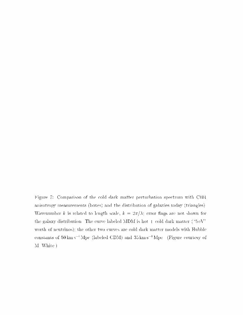
Figure 7: Comparison of the cold dark matter perturbation spectrum with CBR
anisotropy measurements (boxes) and the distribution of galaxies today (triangles).
Wavenumber k is related to length scale, k = 2�=�; error ags are not shown for
the galaxy distribution. The curve labeled MDM is hot + cold dark matter (\5 eV"
worth of neutrinos); the other two curves are cold dark matter models with Hubble
constants of 50 km s�1Mpc (labeled CDM) and 35 km s�1Mpc. (Figure courtesy of
M. White.)

angular scales much greater than about 1� (corresponding to multipoles
l � 100), it is the dominant contribution. It is useful to expand the CBR
temperature on the sky in spherical harmonics,
�T (�; �)
T0=
l=1;m=lXl�2;m=�l
almYlm(�; �); (65)
where T0 = 2:73K is the CBR temperature today, and the dipole term is
subtracted out because it cannot be separated from that arising due to
our motion with respect to the cosmic rest frame. The predicted variance
due to scalar perturbations is given by
hjalmj2i =H40
2�
Z 1
0k�2 PS(k) jjl(kr0)j2 dk; (66)
' A2n�1H40 r
1�n0
16
�(l + 12n� 1
2)�(3� n)
�(l � 12n+ 5
2)[�(2� 1
2n)]2
; (67)
where r0 � 2H�10 is the comoving distance to the last scattering surface,
and this expression is for the Sachs-Wolfe contribution from scalar pertur-
bations only. For n � 1, the expectation for the square of the quadrupole
anisotropy is
��T
T0
�2Q�S
� 5ja2mj24�
� 32�
45
V50
mP l4 x250
(k50r0)1�n: (68)
(By choosing k50 = r�10 = 12H0, the last factor becomes unity.)
The ensemble expectation for the multipole amplitudes is often re-
ferred to as the angular power spectrum because they encode the full
information about predicted CBR anisotropy. For example, the rms tem-
perature uctuation on a given angular scale is related to the multipole
amplitudes ��T
T
�2�
� l2hjalmj2i for l ' 200�=�: (69)
The procedure for specifying the tensor modes is similar, cf. Refs. 71
and 72. For the modes that enter the horizon after the universe becomes
matter dominated, k <� 0:1h2Mpc, which are the only modes that con-

tribute signi�cantly to CBR anisotropy on angular scales greater than a de-
gree,
hik(�) = ai(k)
3j1(k�)
k�
!; (70)
where � = r0(t=t0)1=3 is conformal time. [For the modes that enter the
horizon during the radiation-dominated era, k >� 0:1h2Mpc�1, the factor
3j1(k�)=k� is replaced by j0(k�) for the remainder of the radiation era. In
either case, the factor involving the spherical Bessel function quanti�es the
fact that tensor perturbations remain constant while outside the horizon,
and after horizon crossing, decrease as R�1.]
The tensor perturbations too are characterized by a Gaussian, random
variable, here written as ai(k); the statistical expectation is
hhikhjqi = PT (k)(2�)6�(3)(k � q)�ij ; (71)
where the power spectrum
PT (k) = ATknT�3
"3j1(k�)
k�
#2; (72)
AT =8
3�
V50
mP l4
(1 + 56nT )[�(
32� 1
2nT )]
2
2nT [�(32)]2
k�nT50 ; (73)
where the O(�i) correction to AT has been included. Note that nT =
�2�T is zero for scale-invariant perturbations.
Finally, the contribution of tensor perturbations to the multipole am-
plitudes, which arise solely due to the Sachs-Wolfe e�ect,31,71,72 is given
by
hjalmj2i ' 36�2�(l + 3)
�(l � 1)
Z 1
0knT+1AT jFl(k)j2 dk; (74)
where
Fl(k) = �Z r0
rD
drj2(kr)
kr
"jl(kr0 � kr)
(kr0 � kr)2
#; (75)
and rD = r0=(1 + zD)1=2 � r0=35 is the comoving distance to the horizon
at decoupling (= conformal time at decoupling). Equation (74) is approx-
imate in that very short wavelength modes, kr0 � 100, that crossed inside

the horizon before matter-radiation equality have not been properly taken
into account; to take them into account, the integrand must be multiplied
by a transfer function,
T (k) ' 1:0 + 1:44(k=kEQ) + 2:54(k=kEQ)2; (76)
where kEQ � H0=(2p2 � 2)R
1=2EQ is the scale that entered the horizon at
matter-radiation equality.68 In addition, for l >� 1000, the �nite thickness
of the last-scattering surface must be taken into account.
The tensor contribution to the quadrupole CBR temperature anisotropy
for nT not too di�erent from zero is
��T
T0
�2Q�T
� 5ja2mj24�
' 0:61V50
mP l4(k50r0)
�nT ; (77)
where the integrals in the previous expressions have been evaluated nu-
merically.
Both the scalar and tensor contributions to a given multipole are
dominated by wavenumbers kr0 � l. For scale-invariant perturbations
and small l, both the scalar and tensor contributions to (l + 12)2hjalmj2i
are approximately constant. The contribution of scalar perturbations to
(l + 12)2hjalmj2i begins to decrease for l � 150 because the scalar contri-
bution to these multipoles is dominated by modes that entered the hori-
zon before matter domination (and hence are suppressed by the transfer
function). The contribution of tensor modes to (l + 12)2hjalmj2i begins to
decrease for l � 30 because the tensor contribution to these multipoles
is dominated by modes that entered the horizon before decoupling (and
hence decayed as R�1 until decoupling). Figure 8 shows the contribution
of scalar and tensor perturbations to the CBR anisotropy multipole am-
plitudes (and includes both the tensor and scalar transfer functions); the
expected variance in the CBR multipoles is given by the sum of the scalar
and tensor contributions.

Figure 8: Scalar and tensor contributions to the CBR multipole moments: l (l +
1) hjalmj2i=6hja2mj2i for the scalar and l(l + 12)hjalmj2i=5hja2mj2i for the tensor with
n � 1 = nT = 0, zDEC = 1100, and h = 0:5 (from Ref. 73). (The tensor angular
power spectrum falls o� for l � 30.) Scale invariance manifests itself in the constancy
of the angular power spectra for l <� 100. Note, only the Sachs-Wolfe contribution is
shown; for scalar perturbations, other e�ects become dominant for l >� 100 and the
spectrum rises to a \Doppler peak" at around l � 200, cf. Fig. 3.

3.2 Worked Examples
In this section, I apply the formalism developed in the two previous sec-
tions to four speci�c models. So that I can, where appropriate, solve
numerically for model parameters, I will: (1) assume that the astrophys-
ically interesting scales crossed outside the horizon 50 e-folds before the
end of in ation, and (2) use the COBE DMR quadrupole measurement,
h(�T )2Qi1=2 � 20� 2�K,11,74 to normalize the scalar perturbations; using
Eq. (55), this implies
V50 � 2:3� 10�11m4P l x
250: (78)
Of course, it is entirely possible that a signi�cant portion of the quadrupole
anisotropy is due to tensor-mode perturbations, in which case, this nor-
malizationmust be reduced by a factor of (1+T=S)�1. And, it is straight-
forward to change \50" to the number appropriate to a speci�c model or
to normalize the perturbations another way.
Before going on, let us use the COBE DMR quadrupole anisotropy to
bound the tensor contribution to the quadrupole anisotropy, and thereby,
the energy density that drives in ation:
V50 <� 7� 10�11mP l4: (79)
Thus, the upper limit to the tensor contribution to the CBR quadrupole
implies that the vacuum energy that drives in ation must be much less
than the Planck energy density, indicating that the �nal 50 or so e-foldings
of in ation, which is the relevant part of in ation for us, is not a quantum-
gravitational phenomenon. Of course, in ation could last far longer than
50 e-foldings, and during the earliest part of in ation, the energy density
could be Planckian (this is the point of view advocated by Linde in his
chaotic in ation model46).
3.2.1 Exponential Potentials
There is a class of models that can be described in terms of an exponential
potential,
V (�) = V0 exp(���=mP l): (80)
This type of potential was �rst invoked in the context of power-law in a-
tion75 and has recently received renewed interest in the context of extended
in ation.76 In the simplest model of extended or �rst-order in ation, that
is based upon the Brans-Dicke-Jordan theory of gravity,76 � is related to
the Brans-Dicke parameter: �2 = 64�=(2! + 3).
For such a potential, the slow-roll conditions are satis�ed provided that
�2 <� 24�; thus in ation does not end until the potential changes shape,
or in the case of extended in ation, until the phase transition takes place.
In either case, we can relate �50 to �end,
N(�50) = 50 =8�
mP l2
Z �end
�50
V d�
�V 0; ) �50 = �end � 50�=8�: (81)
Since �end is in e�ect arbitrary, the overall normalization of the potential
is irrelevant. The two other parameters, x50 and x050, are easy to compute:
x50 = ��; x050 = 0: (82)
Using the COBE DMR normalization, we can relate V50 and �:
V50 = 2:3� 10�11mP l4�2: (83)
Further, we can compute q, �S, �T , and T=S:
q = 16�=�2; T=S = 0:28�2; �T = �S = 1=(q � 1) ' �2=16�:
(84)
Note, for the exponential potential, q, �T = �S are independent of epoch.
In the case of extended in ation, �S = �T = 4=(2! + 3); since ! must be
less than about 20 (Ref. 78), this implies signi�cant tilt: �S = �T >� 0:1.

3.2.2 Chaotic In ation
The simplest chaotic in ation models are based upon potentials of the
form:
V (�) = a�b; (85)
b = 4 corresponds to Linde's original model of chaotic in ation, and a is
dimensionless,46 and b = 2 is a model based upon a massive scalar �eld
and m2 = 2a (Ref. 79). In these models, � is initially displaced from
� = 0, and in ation occurs as � slowly rolls to the origin. The value of
�end is easily found: �2end = b(b� 1)mP l
2=24�, and
N(�50) = 50 =8�
mP l2
Z �50
�end
V d�
V 0; (86)
) �250=mP l2 = 50b=4�+ b2=48� ' 50b=4�; (87)
the value of �50 is a few times the Planck mass.
For purposes of illustration, consider b = 4; �end = mP l=p2� '
0:4mP l, �50 ' 4mP l, �46 ' 3:84mP l, and �54 ' 4:16mP l. In order to
have su�cient in ation, the initial value of � must exceed about 4:2mP l;
in ation ends when � � 0:4mP l; and the scales of astrophysical interest
cross outside the horizon over an interval �� ' 0:3mP l.
The values of the potential, its steepness, and the change in steepness
are easily found,
V50 = amP lb
50b
4�
!b=2; x50 =
s4�b
50; mP lx
050 =
�4�50
; (88)
q50 = 200=b; T=S = 0:07b; �T ' b=200; �S = �T + 0:01:
(89)
Unless b is very large, scalar perturbations dominate tensor perturba-
tions,80 �T , �S are very small, and q is very large. Further, when �T , �S
become signi�cant, they are equal. Using the COBE DMR normalization,
we �nd:
a = 2:3� 10�11b1�b=2(4�=50)b=2+1mP l4�b: (90)

For the two special cases of interest: b = 4, a = 9 � 10�14; and b = 2,
m2 � 2a = 3� 10�12mP l2.
3.2.3 New In ation
These models entail a very at potential where the scalar �eld rolls from
� � 0 to the minimum of the potential at � = �. The original models
of slow-rollover in ation81 were based upon potentials of the Coleman-
Weinberg form
V (�) = B�4=2 + B�4�ln(�2=�2)� 1
2
�; (91)
where B is a very small dimensionless coupling constant. Other very at
potentials also work (e.g., V = V0 � ��4 + ��6 [Ref. 47]). As before, we
�rst solve for �50:
N(�50) = 50 =8�
mP l2
Z �50
�end
V d�
V 0; ) �250 =
��4
100j ln(�250=�2)jmP l2;
(92)
where the precise value of �end is not relevant, only the fact that it is much
larger than �50. Provided that � <� mP l, both �50 and �end are much less
than �; we then �nd
V50 ' B�4=2; x50 ' � (�=25)3=2qj ln(�250=�2j)
��
mP l
�2� 1; (93)
mP lx050 ' �24�=100; q50 ' 2:5� 105j ln(�250=�2)j
�2
�mP l
�
�4� 1;
(94)
�T ' 1
q50� 1; �S = �T + 0:03;
T
S' 6� 10�4
j ln(�250=�2)j��
mP l
�4:
(95)
Provided that � <� mP l, x50 is very small; this means that q is very large,
gravity-waves and density perturbations are very nearly scale invariant,
and T=S is small. Finally, using the COBE DMR normalization, we can
determine the dimensionless coupling constant B:
B ' 9� 10�14=j ln(�250=�2)j � 4� 10�15: (96)
3.2.4 Natural In ation
This model is based upon a potential of the form55
V (�) = �4 [1 + cos(�=f)] : (97)
The atness of the potential (and requisite small couplings) arise because
the � particle is a pseudo-Nambu-Goldstone boson (f is the scale of spon-
taneous symmetry breaking and � is the scale of explicit symmetry break-
ing; in the limit that �! 0, the � particle is a massless Nambu-Goldstone
boson). It is a simple matter to show that �end is of the order of �f .
This potential is di�cult to analyze in general; however, there are two
limiting regimes: (i) f � mP l; and (ii) f <� mP l (Ref. 47). In the �rst
regime, the 50 or so relevant e-folds take place close to the minimum of
the potential, � = �f , and in ation can be analyzed by expanding the
potential about � = �,
V ( ) ' m2 2=2; (98)
m2 = �4=f2; = �� �: (99)
In this regime, natural in ation is equivalent to chaotic in ation with
m2 = �4=f2 ' 3� 10�12mP l2.
In the second regime, f <� mP l, in ation takes place when � <� �f ,
so that we can make the following approximations: V ' 2�4 and V 0 =
��4�=f2. Taking �end � �f , we can solve for N(�):
N(�) =8�
mP l2
Z �f
�
V d�
�V 0' 16�mP l
2
f2ln(�f=�); (100)
from which it is clear that achieving 50 e-folds of in ation places a lower
bound to f , very roughly f >� mP l=3 (Refs. 47 and 55).

Now, we can solve for �50, V50, x50, and x050:
�50=�f ' exp(�50mP l2=16�f2) <� O(0:1); V50 ' 2�4; (101)
x50 ' 1
2
mP l
f
�50
f<� O(0:1); x050 ' �
1
2
mP l
f
!2: (102)
Using the COBE DMR normalization, we can relate � to f=mP l:
�=mP l = 7� 10�4smP l
fexp(�25mP l
2=16�f2): (103)
Further, we can solve for T=S, �T , and �S:
T
S' 0:07
mP l
f
!2 �50
f
!2<� O(0:1); (104)
�T =1
16�
q50
q50 � 1
1
4
mP l2
f2�250f2
!� 1
64�
mP l
f
!2 �50
f
!2� 0:1; (105)
�S =1
16�
q50
q50 � 1
1
4
mP l2
f2�250f2
+mP l
2
f2
!� 1
16�
mP l
f
!2; (106)
q50 = 64�
f
mP l
!2 f
�50
!2� 1: (107)
Regime (ii) provides the exception to the rule that �S � �T and large
�S implies large T=S. For example, taking f = mP l=2, we �nd:
�50=f � 0:06; x50 � 0:06; x050 = �2; q50 � 104; (108)
�T � 10�4; �S � 0:08; T=S � 10�3: (109)
The gravitational-wave perturbations are very nearly scale invariant, while
the density perturbations deviate signi�cantly from scale invariance. I
note that regime (ii), i.e., f <� mP l, occupies only a tiny fraction of pa-
rameter space because f must be greater than about mP l=3 to achieve
su�cient in ation; further, regime (ii) is \�ne tuned" and \unnatural"
in the sense that the required value of � is exponentially sensitive to the
value of f=mP l.
Finally, I note that the results for regime (ii) apply to any in ationary
model whose Taylor expansion in the in ationary region is similar; e.g.,
V (�) = �m2�2 + ��4, which was originally analyzed in Ref. 47.

3.2.5 Lessons
To summarize the general features of our results: In all examples, the
deviations from scale invariance enhance perturbations on large scales.
The only potentials that have signi�cant deviations from scale invariance
are either very steep or have rapidly changing steepness. In the former
case, both the scalar and tensor perturbations are tilted by a similar
amount; in the latter case, only the scalar perturbations are tilted.
For \steep" potentials, the expansion rate is \slow," i.e., q50 close to
unity, the gravity-wave contribution to the CBR quadrupole anisotropy
becomes comparable to, or greater than, that of density perturbations,
and both scalar and tensor perturbations are tilted signi�cantly. For at
potentials, i.e., small x50, the expansion rate is \fast," i.e., q50 � 1, the
gravity-wave contribution to the CBR quadrupole is much smaller than
that of density perturbations, and unless the steepness of the potential
changes signi�cantly, large x050, both spectra are very nearly scale invari-
ant; if the steepness of the potential changes rapidly, the spectrum of
scalar perturbations can be tilted signi�cantly. The models that permit
signi�cant deviations from scale invariance involve exponential or low-
order polynomial potentials; the former by virtue of their steepness, the
latter by virtue of the rapid variation of their steepness. Exponential po-
tentials are of interest because they arise in extended in ation models;
potentials with rapidly varying steepness include V (�) = �m2�2+��4 or
�4[1 + cos(�=f)].
Finally, to illustrate how observational data could be used to determine
the properties of the in ationary potential and test the consistency of the
in ationary hypothesis, suppose observations determined the following:
(�T )Q ' 16�K; T=S = 0:24; n = 0:9: (110)
That is, suppose the COBE DMR quadrupole anisotropy holds up, a value
of four-to-one is found for the ratio scalar to tensor contributions to the

CBR quadrupole, and a spectral index of 0.9 for the scalar perturbations.
From T=S, we determine the steepness of the potential: x50 ' 0:94. From
the steepness and the quadrupole anisotropy, the value of the potential:
V1=450 ' 2:4� 1016GeV. From the spectral index, the change in steepness
is: x050 ' �0:81=mP l. These data can also be expressed in terms of the
value of the potential and its �rst two derivatives:
V50 = 1:4� 10�11mP l4; V 0
50 = 1:5� 10�11mP l3; V 00
50 = 1:0� 10�12mP l2:
(111)
Further, they then lead to the prediction: nT = �0:035, which, when\measured," can be used as a consistency check for in ation.
4 Structure Formation: Crucial Test
of In ation
The key to testing in ation is to focus on its robust predictions and their
implications. Earlier, I discussed the prediction of a at universe and its
bold implication that most of the matter in universe exists in the form
of particle dark matter. Much e�ort is being directed at determining the
mean density of the universe and detecting particle dark matter.
The scale-invariant scalarmetric perturbations lead to CBR anisotropy
on angular scales from less than 1� to 90� and seed the formation of struc-
ture in the universe. Together with the nucleosynthesis determination of
B and the in ationary prediction of a at universe, scale-invariant den-
sity perturbations lead to a very speci�c scenario for structure formation;
it is known as cold dark matter because the bulk of the particle dark mat-
ter is comprised of slowly moving particles (e.g., axions or neutralinos).yy82A large and rapidly growing number of observations are being brought to
yyThe simpler possibility, that the particle dark matter exists in the form of 30 eV or so neutrinos,
which is known as hot dark matter, was falsi�ed almost a decade ago. Because neutrinos move
rapidly, they can di�use from high density to low density regions damping perturbations on small

bear in the testing of cold dark matter, making it the centerpiece of e�orts
to test in ation.
Finally, there are the scale-invariant tensor perturbations. They lead
to CBR anisotropy on angular scales from a few degrees to 90� and a spec-
trum of gravitational waves. The CBR anisotropy arising from the tensor
perturbations can in principle be separated from that arising from scalar
perturbations. However, because the sky is �nite, sampling variance sets a
fundamental limit. The tensor contribution to CBR anisotropy can only
be separated from that of the scalar if T=S is greater than about 0:14
(Ref. 83). It is also possible that the stochastic background of gravita-
tional waves itself can be directly detected, though it appears that the
LIGO facilities being built will lack the sensitivity, and even space-based
interferometery (e.g., LISA) is not a sure bet.84
Before going on to discuss how cold dark matter models are testing
in ation, I want to emphasize the importance of the tensor perturbations.
The attractiveness of a at universe with scale-invariant density pertur-
bations was appreciated long before in ation. Verifying these two predic-
tions of in ation, while important, will not provide a \smoking gun." The
tensor perturbations are a unique feature of in ation. Further, they are
crucial to obtaining information about the scalar potential responsible for
in ation.
4.1 Vanilla Cold Dark Matter: Almost, but Not
Quite?
Cold dark matter has often been characterized as a \no parameter model"
for structure formation; that is only true in the broad brush. Cold dark
matter is characterized by scale-invariant density perturbations and a mat-
scales. In hot dark matter, large, supercluster-size objects must form before galaxies, and thus hot
dark matter cannot account for the abundance of galaxies, damped Lyman-� clouds, etc., that is
observed at high redshift.

ter content that is almost entirely slowly moving particles. To make pre-
dictions of the precision needed to match current observations, a more
speci�c characterization is essential|precise power-law index of the spec-
trum of density perturbations, amplitude of tensor perturbations, Hubble
constant, baryon density, radiation content of the universe, possible cos-
mological constant, and so on.
Historically, the \standard" version of cold dark matter, \vanilla cold
dark matter" if you will, is: (1) B ' 0:05 and CDM � 0:95, (2) Hubble
constant of 50 km s�1Mpc�1, (3) precisely scale-invariant density pertur-
bations (n = 1), and (4) no contribution of tensor perturbations to CBR
anisotropy. Standard cold dark matter has no other signi�cance than as a
default starting point. Because it became an \industry standard," vanilla
cold dark matter provides an interesting point of comparison|but that is
all!
In cold dark matter models, structure forms hierarchically, with small
objects forming �rst which then merge to form larger objects. Galaxies
form at redshifts of the order of few, and rarer objects like QSOs form from
higher than average density peaks earlier. In general, cold dark matter
predicts a universe that is still evolving at recent epochs. N -body sim-
ulations are crucial to bridging the gap between theory and observation,
and several groups have carried out large numerical studies of vanilla cold
dark matter.85
There are a diversity of observations that test cold dark matter; they
include CBR anisotropy and spectral distortions, redshift surveys, pair-
wise velocities of galaxies, peculiar velocities, redshift space distortions, x-
ray background, QSO absorption line systems, cluster studies of all kinds,
studies of evolution (clusters, galaxies, and so on), measurements of the
Hubble constant, and on and on. I will focus on how these measurements
probe the power spectrum of density perturbations, emphasizing the role
of CBR-anisotropy measurements and redshift surveys.

Density perturbations on a (comoving) length scale � give rise to CBR
anisotropy on an angular scale � � �=H�10 � 1�(�=100h�1Mpc).zz CBR
anisotropy has now been detected by more than ten experiments on an-
gular scales from about 0:5� to 90�, thereby probing length scales from
30h�1Mpc to 104h�1Mpc. The very accurate measurements made by the
COBE DMR can be used to normalize the cold dark matter spectrum
(the normalization scale corresponds to about 20�). When this is done,
the other ten or so measurements are in agreement with the predictions
of cold dark matter (see Fig. 1).
The COBE-normalized cold dark matter spectrum can be extrapo-
lated to the much smaller scales probed by redshift surveys, from about
1h�1Mpc to 100h�1Mpc. When this is done, there is general agreement.
However, on closer inspection, the COBE-normalized spectrum seems to
predict excess power on these scales (about a factor of four in the power
spectrum; see Fig. 7). This conclusion is supported by other observations,
e.g., the abundance of rich clusters and the pairwise velocities of galaxies.
It suggests that cold dark matter has much of the truth, but perhaps not
all of it,86 and has led to the suggestion that something needs to be added
to the simplest cold dark matter theory.
There is another important challenge facing cold dark matter. X-
ray observations of rich clusters are able to determine the ratio of hot gas
(baryons) to total cluster mass (baryons + CDM) (by a wide margin, most
of the baryons \seen" in clusters are in the hot gas). To be sure, there
are assumptions and uncertainties; the data at the moment indicate that
this ratio is (0:04� 0:08)h�3=2 (Ref. 22). If clusters provide a fair sample
of the universal mix of matter, then this ratio should equal B=(B +
CDM) ' (0:009 � 0:022)h�2=(B + CDM). Since clusters are large
objects, they should provide a pretty fair sample. Taking the numbers
zzFor reference, perturbations on a length scale of about 1Mpc give rise to galaxies, on about 10Mpc
to clusters, on about 30Mpc to large voids, and on about 100Mpc to the great walls.
at face value, cold dark matter is consistent with the cluster gas fraction
provided either: B + CDM = 1 and h � 0:3 or B + CDM � 0:3 and
h � 0:7. The cluster baryon problem has yet to be settled and is clearly
an important test of cold dark matter.
Finally, before going on to discuss the variants of cold dark matter
now under consideration, let me add a note of caution. The comparison
of predictions for structure formation with present-day observations of the
distribution of galaxies is fraught with di�culties. Theory most accurately
predicts \where the mass is" (in a statistical sense) and the observations
determine where the light is. Redshift surveys probe present-day inho-
mogeneity on scales from around one Mpc to a few hundred Mpc, scales
where the universe is nonlinear (�nGAL=nGAL >� 1 on scales <� 8h�1Mpc)
and where astrophysical processes undoubtedly play an important role
(e.g., star formation determines where and when \mass lights up;" the
explosive release of energy in supernovae can move matter around and
in uence subsequent star formation, and so on). The distance to a galaxy
is determined through Hubble's law (d = H�10 z) by measuring a redshift;
peculiar velocities induced by the lumpy distribution of matter are sig-
ni�cant and prevent a direct determination of the actual distance. There
are the intrinsic limitations of the surveys themselves|they are ux, not
volume, limited (brighter objects are seen to greater distances and vice
versa) and relatively small (e.g., the CfA slices of the universe survey con-
tains only about 104 galaxies and extends to a redshift of about z � 0:03).
Last but not least are the numerical simulations which link theory and
observation; they are limited in dynamical range (about a factor of 100 in
length scale) and in microphysics (in the largest simulations, only gravity,
and in others, only a gross approximation to the e�ects of hydrodynam-
ics/thermodynamics). Perhaps it would be prudent to withhold judgment
on vanilla cold dark matter for the moment and resist the urge to modify
it|but that wouldn't be as much fun!

4.2 The Many Flavors of Cold Dark Matter
The spectrum of density perturbations today depends not only upon the
primeval spectrum (and the normalization on large scales provided by
COBE), but also upon the energy content of the universe. While the
uctuations in the gravitational potential were initially (approximately)
scale invariant, the universe evolved from an early radiation-dominated
phase to a matter-dominated phase which imposes a characteristic scale on
the spectrum of density perturbations seen today; that scale is determined
by the energy content of the universe, kEQ � 10�1hMpc�1 (matterh=pg�)
(g� counts the relativistic degrees of freedom, matter = B + CDM). In
addition, if some of the nonbaryonic dark matter is neutrinos, they reduce
power on small scales somewhat through free-streaming (see Fig. 7). With
this in mind, let me discuss the variants of cold dark matter that have
been proposed to improve its agreement with observations.
1. Low Hubble constant + cold dark matter (LHC CDM).87 Re-
markably, simply lowering the Hubble constant to around 30 km s�1
Mpc�1 solves all the problems of cold dark matter. Recall, the crit-
ical density �crit / H20 ; lowering H0 lowers the matter density and
has precisely the desired e�ect. It has two other added bene�ts: the
expansion age of the universe is comfortably consistent with the ages
of the oldest stars, and the baryon fraction is raised to a value that
is consistent with that measured in x-ray clusters. Needless to say,
such a small value for the Hubble constant ies in the face of current
observations;5,6 further, it illustrates that the problems of cold dark
matter get even worse for the larger values of H0 that are favored by
recent observations.
2. Hot + cold dark matter (�CDM).88 Adding a small amount of
hot dark matter can suppress density perturbations on small scales;
adding too much leads back to the longstanding problems of hot dark
matter. Retaining enough power on very small scales to produce
damped Lyman-� systems at high redshift limits � to less than
about 20%, corresponding to about 5 eV worth of neutrinos (i.e., one
species of mass 5 eV, or two species of mass 2:5 eV, and so on). This
admixture of hot dark matter rejuvenates cold dark matter provided
the Hubble constant is not too large, H0<� 55 km s�1Mpc�1; in fact,
a Hubble constant of closer to 45 km s�1Mpc�1 is preferred.
3. Cosmological constant + cold dark matter (�CDM).89 (A
cosmological constant corresponds to a uniform energy density or
vacuum energy.) Shifting 50% to 70% of the critical density to a
cosmological constant lowers the matter density and has the same
bene�cial e�ect as a low Hubble constant. In fact, a Hubble constant
as large as 80 km s�1Mpc�1 can be accommodated. In addition, the
cosmological constant allows the age problem to be solved even if
the Hubble constant is large, addresses the fact that few measure-
ments of the mean mass density give a value as large as the critical
density (most measurements of the mass density are insensitive to a
uniform component), and allows the baryon fraction of matter to be
larger, which alleviates the cluster baryon problem. Not everything
is rosy; cosmologists have invoked a cosmological constant twice be-
fore to solve their problems (Einstein to obtain a static universe and
Bondi, Gold, and Hoyle to solve the earlier age crisis when H0 was
thought to be 250 km s�1Mpc�1). Further, particle physicists can
still not explain why the energy of the vacuum is not at least 50 (if
not 120) orders of magnitude larger than the present critical density
and expect that when the problem is solved, the answer will be zero.
4. Extra relativistic particles + cold dark matter (�CDM).90
Raising the level of radiation has the same bene�cial e�ect as low-
ering the matter density. In the standard cosmology, the radiation
content consists of photons + three (undetected) cosmic seas of neu-

trinos (corresponding to g� ' 3:36). While we have no direct deter-
mination of the radiation beyond that in the CBR, there are at least
two problems: What are the additional relativistic particles? Can
additional radiation be added without upsetting the successful pre-
dictions of primordial nucleosynthesis which depend critically upon
the energy density of relativistic particles? The simplest way around
these problems is an unstable tau neutrino (mass anywhere between
a few keV and a few MeV) whose decays produce the radiation. This
�x can tolerate a larger Hubble constant, though at the expense of
more radiation.
5. Tilted cold dark matter (TCDM).91 While the spectrum of den-
sity perturbations in most models of in ation is very nearly scale
invariant, there are models where the deviations are signi�cant (n �0:8) which leads to smaller uctuations on small scales. Further, if
gravity waves account for a signi�cant part of the CBR anisotropy,
the level of density perturbations can be lowered even more. A com-
bination of tilt and gravity waves can solve the problem of too much
power on small scales but seems to lead to too little power on inter-
mediate and very small scales.
These possibilities represent di�erent approaches to improving the con-
cordance of CDM. They also represent well-motivatedmodi�cations to the
standard cosmology in their own right. It has always been appreciated
that the in ationary spectrum of density perturbations was not exactly
scale invariant47 and that the Hubble constant was unlikely to be exactly
50 km s�1Mpc. Neutrinos exist; they are expected to have mass; there is
even some experimental data that indicates they do have mass.92 If the
Hubble constant is as large as 70 km s�1Mpc�1 to 80 km s�1Mpc�1, a cos-
mological constant seems inescapable based upon the age of the universe
alone. There is no data that precludes more radiation than in the standard
cosmology. In fact, these modi�cations to vanilla cold dark matter are so

well-motivated that one should probably also consider combinations; e.g.,
lesser tilt and h = 0:45 and so on.93
In evaluating these better �t models, one should keep the words of
Francis Crick in mind (loosely paraphrased): A model that �ts all the
data at a given time is necessarily wrong, because at any given time,
not all the data are correct(!). �CDM provides an interesting/confusing
example. When I discussed it in 1990, I called it the best-�t universe, and
quoting Crick, I said that �CDM was certain to fall by the wayside.94 In
1995, it is still the best-�t model.95
4.3 Reconstruction
If in ation and the cold dark matter theory is shown to be correct, then a
window to the very early universe (t � 10�34 sec) will have been opened.
While it is certainly premature to jump to this conclusion, I would like
to illustrate one example of what one could hope to learn. As mentioned
earlier, the spectra and amplitudes of the the tensor and scalar metric
perturbations predicted by in ation depend upon the underlying model,
to be speci�c, the shape of the in ationary scalar-�eld potential. If one
can measure the power-law index of the scalar spectrum and the ampli-
tudes of the scalar and tensor spectra, one can recover the value of the
potential and its �rst two derivatives around the point on the potential
where in ation took place:96
V = 1:65T mPl4; (112)
V 0 = �s8�r
7V=mPl; (113)
V 00 = 4��(n� 1) +
3
7r
�V=mPl
2; (114)
where r � T=S, a prime indicates derivative with respect to �, mP l =
1:22� 1019GeV is the Planck energy, and the sign of V 0 is indeterminate.
In addition, if the tensor spectral index can be measured, a consistency
relation, nT = �r=7, can be used to further test in ation. Reconstruction
of the in ationary scalar potential would shed light both on in ation as
well as physics at energies of the order of 1015GeV. (If � 6= 0, these
expressions are modi�ed.97)
5 The Future
The stakes for cosmology are high: if correct, in ation/cold dark matter
represents a major extension of the Big Bang and our understanding of
the universe. Further, it will shed light on the fundamental physics at
energies of order 1015GeV.
What are the crucial tests and when will they be carried out? Be-
cause of the many measurements/observations that can have signi�cant
impact, I believe the answer to when is sooner rather than later. The
list of pivotal observations is long: CBR anisotropy, large redshift sur-
veys (e.g., the Sloan Digital Sky Survey will have 106 redshifts), direct
searches for nonbaryonic dark matter in our neighborhood (both for axions
and neutralinos) and baryonic dark matter (microlensing), x-ray studies
of galaxy clusters, the use of back-lit gas clouds (quasar absorption line
systems) to study the universe at high redshift, evolution (as revealed
by deep images of the sky taken by the Hubble Space Telescope and the
Keck 10-m telescope), measurements of both H0 and q0, mapping of the
peculiar velocity �eld at large redshifts through the Sunyaev-Zel'dovich
e�ect, dynamical estimates of the mass density (using weak gravitational
lensing, large-scale velocity �elds, and so on), age determinations, gravita-
tional lensing, searches for supersymmetric particles (at accelerators) and
neutrino oscillations (at accelerators, solar-neutrino detectors, and other
large underground detectors), searches for high-energy neutrinos from neu-
tralino annihilations in the sun using large underground detectors, and on

and on. Let me end by illustrating the interesting consequences of sev-
eral possible measurements.
A de�nitive determination that H0 is greater than 55 km s�1Mpc�1
would falsify all CDM models except that with a cosmological constant
and would certainly give particle theorists something to think about. (A
de�nitive determination that H0 is 75 km s�1Mpc�1 or larger would neces-
sitate a cosmological constant based upon the age of the universe alone,
though it should be noted that none of the CDM models consistent with
large-scale structure have an age problem.) A at universe with a cosmo-
logical constant has a very di�erent deceleration parameter than one dom-
inated by matter, q0 = �1:5�+0:5 � �(0:4�0:7) compared to q0 = 0:5,
and this could be settled by galaxy-number counts, quasar-lensing statis-
tics, or a Hubble diagram based upon Type Ia supernovae. The predicted
CBR anisotropy on the 0:5� scale in �CDM and LHC CDM is about 50%
larger than vanilla CDM and about 50% smaller in TCDM, which should
be easily discernible. If neutrino-oscillation experiments were to provide
evidence for a neutrino of mass 5 eV (or two of mass 2:5 eV), �CDM would
seem almost inescapable.92
More CBR measurements are in progress, and there should be many
interesting results in the next few years. In the wake of the success of
COBE, there are proposals, both in the U.S. and Europe, for a satellite-
borne instrument to map the CBR sky with a factor of 30 or more better
resolution. A map of the CBR with 0:3� resolution could separate the
gravity-wave contribution to CBR anisotropy and provide evidence for the
third robust prediction of in ation, as well as determining other important
parameters,98 e.g., the scalar and tensor indices, �, and even 0 (the
position of the \Doppler" peak scales asp0 degrees
99).
The future in cosmology is very bright. We have a highly successful
standard model|the hot Big Bang; bold ideas for extending it|in ation
and cold dark matter; and a ood of data to test these ideas.

References
[1] For a textbook treatment of the standard cosmology, see e.g.,S. Weinberg, Gravitation and Cosmology (Wiley, New York,1972); E. W. Kolb and M. S. Turner, The Early Universe(Addison-Wesley, Redwood City, CA, 1990).
[2] A. Sandage, Physica Scripta T 43, 22 (1992).
[3] J. Mould et al., Astrophys. J. 383, 467 (1991).
[4] See e.g., M. Rowan-Robinson, The Cosmological Distance Lad-der (Freeman, San Francisco, 1985).
[5] M. Fukugita, C. J. Hogan, and P. J. E. Peebles, Nature 366,309 (1993); G. Jacoby et al., Proc. Astron. Soc. Pac. 104, 599(1992); A. Reiss, R. P. Krishner, and W. Press, Astrophys. J.438, L17 (1995); M. Hamuy et al., Astron. J. 109, 1 (1995).
[6] W. Freedman et al., Nature 371, 757 (1994).
[7] J. Mather et al., Astrophys. J. 420, 439 (1993).
[8] P. J. E. Peebles, D. N. Schramm, E. Turner, and R. Kron,Nature 352, 769 (1991).
[9] G. F. Smoot et al., Astrophys. J. 396, L1 (1992); A. Kogutet al., ibid. 419, 1 (1993).
[10] G. F. Smoot, in First Course in Current Topics in Astrofunda-mental Physics, edited by N. Sanchez and A. Zichichi (WorldScienti�c, Singapore, 1992), p. 192.
[11] G. F. Smoot et al., Astrophys. J. 396, L1 (1992); E. L. Wright,ibid. 396, L3 (1992).
[12] M. White, D. Scott, and J. Silk, Ann. Rev. Astron. Astrophys.32, 319 (1994); Science 268, 829 (1995).
[13] T. P. Walker et al., Astrophys. J. 376, 51 (1991).
[14] C. Copi, D. N. Schramm, and M. S. Turner, Science 267, 192(1995).
[15] L. M. Krauss and P. Kernan, Phys. Lett. B 347, 347 (1995).
[16] C. Copi, D. N. Schramm, and M. S. Turner, Phys. Rev. Lett.75, 3981 (1995).
[17] E. W. Kolb et al., Phys. Rev. Lett. 67, 533 (1991).
[18] S. Dodelson, G. Gyuk, and M. S. Turner, Phys. Rev. D 49,5068 (1994).
[19] See e.g., M. Bolte and C. J. Hogan, Nature 376, 399 (1995);J. Cowan, F. Thieleman, and J. Truran, Ann. Rev. Astron.Astrophys. 29, 447 (1991).

[20] For recent reviews of dark matter, see e.g., M. S. Turner, Phys-ica Scripta T 36, 167 (1991); P. J. E. Peebles, Nature 321,27 (1986); V. Trimble, Ann. Rev. Astron. Astrophys. 25, 425(1987); J. Kormendy and G. Knapp, Dark Matter in the Uni-verse (Reidel, Dordrecht, 1989); K. Ashman, Proc. Astron. Soc.Pac. 104, 1109 (1992); S. Faber and J. Gallagher, Ann. Rev.Astron. Astrophys. 17, 135 (1979).
[21] See e.g., N. Kaiser, astro-ph/9509019 (1995).
[22] S. D. M. White et al., Nature 366, 429 (1993); U. G. Brielet al., Astron. Astrophys. 259, L31 (1992); D. A. White andA. C. Fabian, Mon. Not. R. Astron. Soc. 273, 72 (1995).
[23] M. Rowan-Robinson et al., Mon. Not. R. Astr. Soc. 247, 1(1990); N. Kaiser et al., ibid. 252, 1 (1991); M. Strauss et al.,Astrophys. J. 385, 444 (1992).
[24] A. Dekel, Ann. Rev. Astron. Astrophys. 32, 319 (1994).
[25] A. Sandage, Astrophys. J. 133, 355 (1961); Physica ScriptaT43, 7 (1992); Ref. 1.
[26] E. Loh and E. Spillar, Astrophys. J. 307, L1 (1986);M. Fukugita et al., ibid. 361, L1 (1990).
[27] See e.g., E. W. Kolb and M. S. Turner, Ann. Rev. Nucl. Part.Sci. 33, 645 (1983); A. Dolgov, Phys. Repts., in press (1993);A. Cohen, D. Kaplan, and A. Nelson, Ann. Rev. Nucl. Part.Sci. 43, 27 (1992).
[28] S. Weinberg, Gravitation and Cosmology (Wiley, New York,1972).
[29] For a more complete pedagogical discussion of structure forma-tion, see e.g., Ref. 1; P. J. E. Peebles, The Large-Scale Struc-ture of the Universe (Princeton Univ. Press, Princeton, 1980);G. Efstathiou, in The Physics of the Early Universe, edited byJ. A. Peacock, A. F. Heavens, and A. T. Davies (Adam-Higler,Bristol, 1990).
[30] For a pedagogical discussion of CBR anisotropy, see e.g., G. Ef-stathiou, in The Physics of the Early Universe, edited byJ. A. Peacock, A. F. Heavens, and A. T. Davies (Adam-Higler,Bristol, 1990). Also see, J. R. Bond and G. Efstathiou, Mon.Not. R. Astr. Soc. 226, 655 (1987); J. R. Bond et al., Phys.Rev. Lett. 66, 2179 (1991).
[31] R. K. Sachs and A. M. Wolfe, Astrophys. J. 147, 73 (1967).
[32] W. Hu and N. Sugiyama, Phys. Rev. D 51, 2599 (1995).
[33] P. J. E. Peebles, Nature 327, 210 (1987); Astrophys. J. 315,L73 (1987); R. Cen, J. P. Ostriker, and P. J. E. Peebles, ibid.415, 423 (1993).
[34] See e.g., A. Vilenkin, Phys. Repts. 121, 263 (1985); A. Al-brecht and A. Stebbins, Phys. Rev. Lett. 69, 2615 (1992);D. Bennett, A. Stebbins, and F. Bouchet, Astrophys. J. 399,L5 (1992).
[35] See e.g., N. Turok, Phys. Rev. Lett. 63, 2652 (1989); A. Good-ing, D. Spergel, and N. Turok, Astrophys. J. 372, L5 (1991).
[36] C. B. Collins and S. W. Hawking, Astrophys. J. 180, 317(1973).
[37] E. W. Kolb and M. S. Turner, The Early Universe (Addison-Wesley, Redwood City, CA, 1990).
[38] Y. Hu, M. S. Turner, and E. J. Weinberg, Phys. Rev. D 49,3830 (1994).
[39] A. H. Guth and S.-Y. Pi, Phys. Rev. Lett. 49, 1110 (1982);S. W. Hawking, Phys. Lett. B 115, 295 (1982); A. A. Starobin-skii, ibid. 117, 175 (1982); J. M. Bardeen, P. J. Steinhardt, andM. S. Turner, Phys. Rev. D 28, 697 (1983).
[40] V. A. Rubakov, M. Sazhin, and A. Veryaskin, Phys. Lett. B115, 189 (1982); R. Fabbri and M. Pollock, ibid. 125, 445(1983); A. A. Starobinskii, Sov. Astron. Lett. 9, 302 (1983);L. Abbott and M. Wise, Nucl. Phys. B 244, 541 (1984).
[41] M. S. Turner and L. M. Widrow, Phys. Rev. Lett. 57, 2237(1986); L. Jensen and J. Stein-Schabes, Phys. Rev. D 35, 1146(1987); A. A. Starobinskii, JETP Lett. 37, 66 (1983).
[42] A. D. Linde, In ation and Quantum Cosmology (AcademicPress, San Diego, 1990).
[43] A. H. Guth, Phys. Rev. D 23, 347 (1981).
[44] A. D. Linde, Phys. Lett. B 108, 389 (1982).
[45] A. Albrecht and P. J. Steinhardt, Phys. Rev. Lett. 48, 1220(1982).
[46] A. D. Linde, Phys. Lett. B 129, 177 (1983).
[47] P. J. Steinhardt and M. S. Turner, Phys. Rev. D 29, 2162(1984).
[48] Q. Sha� and A. Vilenkin, Phys. Rev. Lett. 52, 691 (1984);S.-Y. Pi, ibid. 52, 1725 (1984).
[49] R. Holman, P. Ramond, and G. G. Ross, Phys. Lett. B 137,343 (1984).
[50] K. Olive, Phys. Repts. 190, 309 (1990).
[51] H. Murayama et al., Phys. Rev. D(RC) 50, R2356 (1994).
[52] M. Cvetic, T. Hubsch, J. Pati, and H. Stremnitzer,Phys. Rev. D 40, 1311 (1990).
[53] E. J. Copeland et al., Phys. Rev. D 49, 6410 (1994).
[54] See e.g., M. Gasperini and G. Veneziano, Phys. Rev. D 50, 2519(1994); R. Brustein and G. Veneziano, Phys. Lett. B 329, 429(1994); T. Banks et al., hep-th/9503114 (1995).
[55] K. Freese, J. A. Frieman, and A. Olinto, Phys. Rev. Lett. 65,3233 (1990).
[56] L. Knox and M. S. Turner, Phys. Rev. Lett. 70, 371 (1993).
[57] J. Silk and M. S. Turner, Phys. Rev. D 35, 419 (1986);L. A. Kofman, A. D. Linde, and J. Einsato, Nature 326, 48(1987).
[58] D. La and P. J. Steinhardt, Phys. Rev. Lett. 62, 376 (1991).
[59] E. W. Kolb, Physica Scripta T36, 199 (1991).
[60] M. Bucher, A. S. Goldhaber, and N. Turok, hep-ph/9411206(1994).
[61] M. S. Turner and F. Wilczek, Phys. Rev. Lett. 65, 3080 (1990);A. Kosowsky, M. S. Turner, and R. Watkins, ibid. 69, 2026(1992).
[62] M. S. Turner and L. M. Widrow, Phys. Rev. D 37, 2743 (1988);B. Ratra, Astrophys. J. 391, L1 (1992).
[63] See e.g., A. D. Linde, Phys. Lett. B 158, 375 (1985); D. Seckeland M. S. Turner, Phys. Rev. D 32, 3178 (1985); M. S. Turner,A. Cohen, and D. Kaplan, Phys. Lett. B 216, 20 (1989).
[64] A. Albrecht et al., Phys. Rev. Lett. 48, 1437 (1982); L. Abbottand M. Wise, Phys. Lett. B 117, 29 (1992); A. D. Linde andA. D. Dolgov, ibid. 116, 329 (1982).
[65] At �rst sight, �rst-order in ation might seem very di�erentfrom slow-rollover in ation, as reheating occurs through the nu-cleation of percolation of true-vacuum bubbles. However, suchmodels can be recast as slow-rollover in ation by means of aconformal transformation, and the analysis of metric perturba-tions proceeds as in slow rollover in ation. See e.g., E. W. Kolb,D. Salopek, and M. S. Turner, Phys. Rev. D 42, 3925 (1990).
[66] E. W. Kolb and M. S. Turner, The Early Universe (Addison-Wesley, Redwood City, CA, 1990), Ch. 8.
[67] E. R. Harrison, Phys. Rev. D 1, 2726 (1970); Y. B. Zel'dovich,Mon. Not. R. Astr. Soc. 160, 1 (1972).
[68] The material presented in this section is a summary ofM. S. Turner, Phys. Rev. D 48, 3502 (1993); ibid., 5539 (1993).
[69] J. M. Bardeen et al., Astrophys. J. 304, 15 (1986).
[70] D. H. Lyth and E. D. Stewart, Phys. Lett. B 274, 168 (1992);E. D. Stewart and D. H. Lyth, ibid. 302, 171 (1993).

[71] L. Abbott and M. Wise, Nucl. Phys. B 244, 541 (1984).
[72] M. White, Phys. Rev. D 46, 4198 (1992).
[73] M. S. Turner, J. E. Lidsey, and M. White, Phys. Rev. D 48,4613 (1993).
[74] E. F. Bunn, D. Scott, and M. White, Astrophys. J. 441, L9(1995).
[75] L. Abbott and M. Wise, Nucl. Phys. B 244, 541 (1984);F. Lucchin and S. Mattarese, Phys. Rev. D 32, 1316 (1985);R. Fabbri, F. Lucchin, and S. Mattarese, Phys. Lett. B 166,49 (1986).
[76] D. La and P. J. Steinhardt, Phys. Rev. Lett. 62, 376 (1989).
[77] E. W. Kolb, D. Salopek, and M. S. Turner, Phys. Rev. D 42,3925 (1990).
[78] E. J. Weinberg, Phys. Rev. D 40, 3950 (1989); M. S. Turner,E. J. Weinberg, and L. Widrow, ibid. 46, 2384 (1992).
[79] V. Belinsky, L. Grishchuk, I. Khalatanikov, andY. B. Zel'dovich, Phys. Lett. B 155, 232 (1985); L. Jensen,1985 (unpublished).
[80] A. A. Starobinskii, Sov. Astron. 11, 133 (1985).
[81] A. D. Linde, Phys. Lett. B 108, 389 (1982); A. Albrecht andP. J. Steinhardt, Phys. Rev. Lett. 48, 1220 (1982).
[82] For an overview of the cold dark matter scenario of structureformation, see e.g., G. Blumenthal et al., Nature 311, 517(1984).
[83] L. Knox and M. S. Turner, Phys. Rev. Lett. 73, 3347 (1994).
[84] M. S. Turner, J. Lidsey, and M. White, Phys. Rev. D 48, 4613(1993).
[85] See e.g., C. Frenk, Physica Scripta T 36, 70 (1991).
[86] See e.g., J. P. Ostriker, Ann. Rev. Astron. Astrophys. 31, 689(1993); A. Liddle and D. Lyth, Phys. Rep. 231, 1 (1993).
[87] J. Bartlett et al., Science 267, 980 (1995).
[88] Q. Sha� and F. Stecker, Phys. Rev. Lett. 53, 1292 (1984);S. Achilli, F. Occhionero, and R. Scaramella, Astrophys. J. 299,577 (1985); S. Ikeuchi, C. Norman, and Y. Zahn, Astrophys. J.324, 33 (1988); A. van Dalen and R. K. Schaefer, Astrophys. J.398, 33 (1992); M. Davis, F. Summers, and D. Schlegel, Nature359, 393 (1992); J. Primack et al., Phys. Rev. Lett. 74, 2160(1995); D. Pogosyan and A. A. Starobinskii, astro-ph/9502019(1995).
[89] M. S. Turner, G. Steigman, and L. Krauss, Phys. Rev. Lett. 52,2090 (1984); M. S. Turner, Physica Scripta T 36, 167 (1991);P. J. E. Peebles, Astrophys. J. 284, 439 (1984); G. Efstathiouet al., Nature 348, 705 (1990); L. Kofman and A. A. Starobin-skii, Sov. Astron. Lett. 11, 271 (1985).
[90] S. Dodelson, G. Gyuk, and M. S. Turner, Phys. Rev. Lett 72,3578 (1994); J. R. Bond and G. Efstathiou, Phys. Lett. B 265,245 (1991).
[91] R. Cen, N. Gnedin, L. Kofman, and J. P. Ostriker, ibid. 399,L11 (1992); R. Davis et al., Phys. Rev. Lett. 69, 1856 (1992);F. Lucchin, S. Mattarese, and S. Mollerach, Astrophys. J. 401,L49 (1992); D. Salopek, Phys. Rev. Lett. 69, 3602 (1992);A. Liddle and D. Lyth, Phys. Lett. B 291, 391 (1992);J. E. Lidsey and P. Coles, Mon. Not. R. Astron. Soc. 258,57 (1992); T. Souradeep and V. Sahni, Mod. Phys. Lett. A 7,3541 (1992).
[92] See e.g., S. Parke, Phys. Rev. Lett. 74, 839 (1995); C. Athanas-sopoulos et al., ibid. 75, 2650 (1995); J. E. Hill, ibid., 2654(1995); K. S. Hirata et al., Phys. Lett. B 280, 146 (1992);Y. Fukuda et al., ibid. 335, 237 (1994); R. Becker-Szendy et al.,Phys. Rev. D 46, 3720 (1992).
[93] M. White, D. Scott, J. Silk, and M. Davis, astro-ph/9508009(to appear in Mon. Not. R. Astron. Soc.) (1995).
[94] M. S. Turner, Physica Scripta T 36, 167 (1991).
[95] L. Krauss and M. S. Turner, astro-ph/9504003 (to appear inGen. Rel. Grav. [1995]).
[96] E. J. Copeland, E. W. Kolb, A. R. Liddle, and J. E. Lid-sey, Phys. Rev. Lett. 71, 219 (1993); Phys. Rev. D 48, 2529(1993); M. S. Turner, ibid., 3502 (1993); ibid. 48, 5539 (1993);A. R. Liddle and M. S. Turner, Phys. Rev. D 50, 758 (1994).
[97] A. R. Liddle, M. S. Turner, and M. White, to be submitted toPhys. Rev. D (1995).
[98] L. Knox, Phys. Rev. D 52, 4307 (1995).
[99] M. Kamionkowski et al., Astrophys. J. 426, L57 (1994);G. Jungman, M. Kamionkowski, A. Kosowsky, andD. N. Spergel, astro-ph/9507080 (1995).