1

High Performance Multiscale Simulation for Crack Propagation

HPSEC 2006 - 18th August

Guillaume Anciaux, Olivier Coulaud and Jean Roman

ScAlApplix Project

2

Outline

1. Introduction

• Motivations

• State of the art

2. Our Approach

• Presentation of the method

• Coupling Algorithm

• Parallel algorithms and implementation

3. Results

• 1D & 2D case : wave propagations

• 2D case : crack

4.Conclusion

3

Introduction

4

Introduction : context

Collaboration with the CEA DIF-DPTA - G. Zerah

Goals : produce a tool for

• CEA1. Better understanding of miscroscale phenomena2. Reduce computing time of molecular dynamics simulations

• ScAlApplix1. Analysis of coupling algorithms2. HPC parallel scaling processes3. Development of a framework for multiscale computation4. Generics : use of legacy codes

Impact on laser optics

5

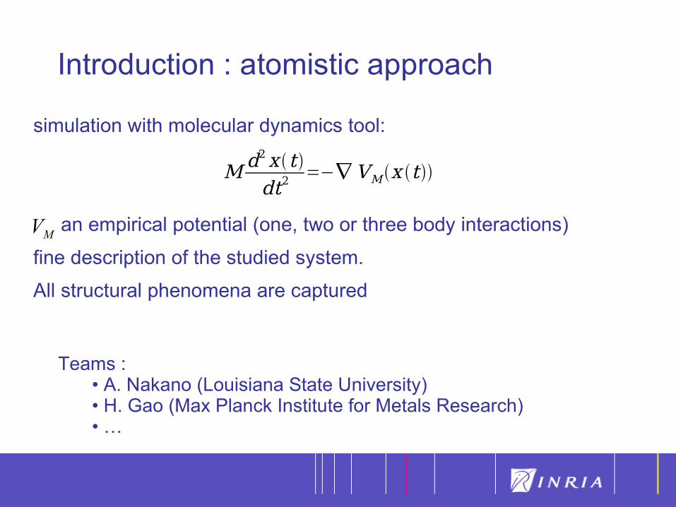
Introduction : atomistic approach

simulation with molecular dynamics tool:

an empirical potential (one, two or three body interactions)

fine description of the studied system.

All structural phenomena are captured

MV

Teams :• A. Nakano (Louisiana State University)• H. Gao (Max Planck Institute for Metals Research)• …

Md2x tdt2

=− VM x t

6

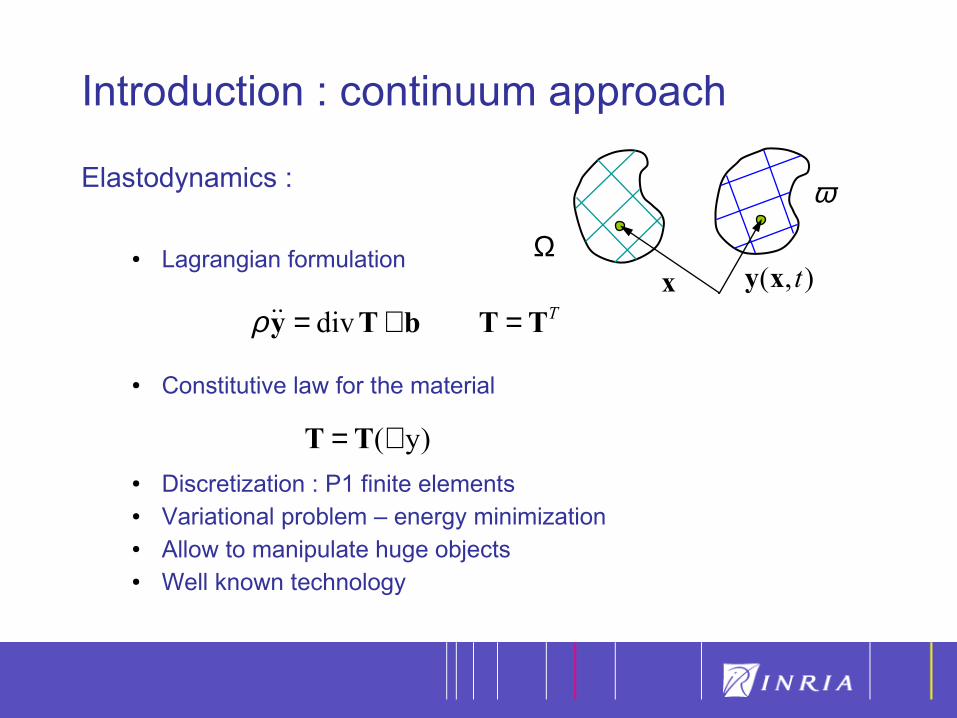
Introduction : continuum approach

Elastodynamics :

Lagrangian formulation

Constitutive law for the material

Discretization : P1 finite elements Variational problem – energy minimization Allow to manipulate huge objects Well known technology

TTTbTy =+= divρ

)y(∇= TT

xΩ

),( txy

ω

7

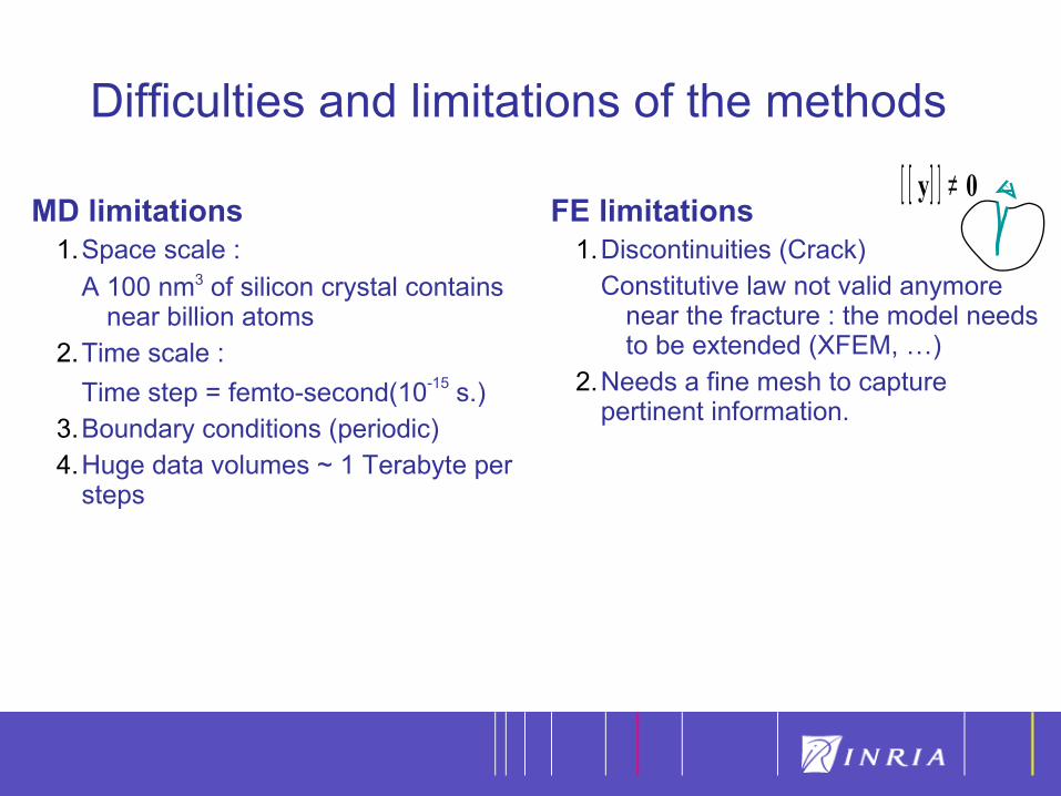
Difficulties and limitations of the methods

MD limitations1.Space scale :

A 100 nm3 of silicon crystal contains near billion atoms

2.Time scale :

Time step = femto-second(10-15 s.)3.Boundary conditions (periodic)4.Huge data volumes ~ 1 Terabyte per

steps

FE limitations1.Discontinuities (Crack)

Constitutive law not valid anymore near the fracture : the model needs to be extended (XFEM, …)

2.Needs a fine mesh to capture pertinent information.

[ [ ] ] 0y ≠

8

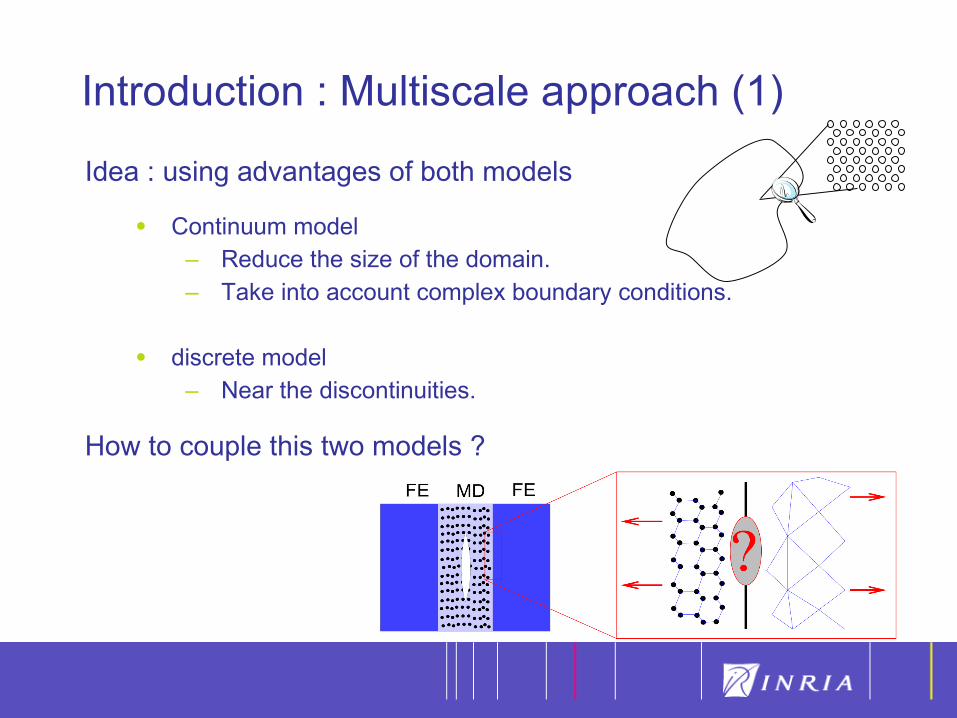
Introduction : Multiscale approach (1)

Idea : using advantages of both models

• Continuum model– Reduce the size of the domain.– Take into account complex boundary conditions.

• discrete model– Near the discontinuities.

How to couple this two models ?

9

Introduction : Multiscale approach (2)

Multi-scale approaches :

• Junction– QC-method (Tadmor and al. 1996)

Static simulations and T= 0 – Macroscopic, Atomistic and Ab initio Dynamics (MAAD) (Abraham

and al. 1998)

• Bridging : duplication of the data– T. Belytschko (Bridging Method)– Bridging Scale Method (Liu)

10

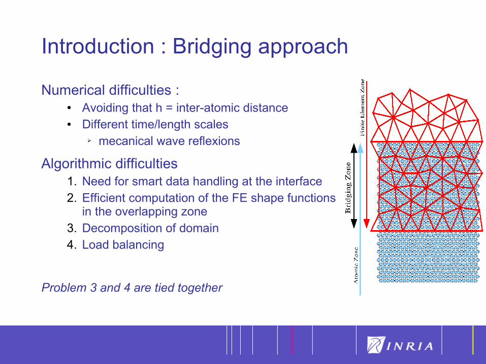
Introduction : Bridging approach

Numerical difficulties : Avoiding that h = inter-atomic distance Different time/length scales

mecanical wave reflexions

Algorithmic difficulties1. Need for smart data handling at the interface2. Efficient computation of the FE shape functions

in the overlapping zone3. Decomposition of domain4. Load balancing

Problem 3 and 4 are tied together

11

Our approach

12

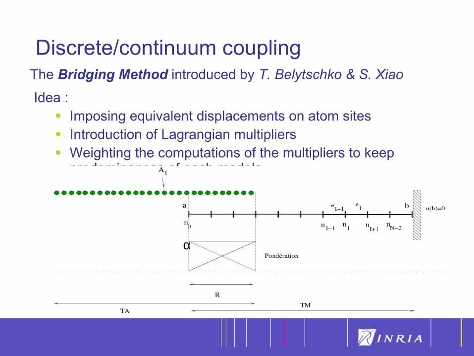
Discrete/continuum couplingThe Bridging Method introduced by T. Belytschko & S. Xiao

Idea :

• Imposing equivalent displacements on atom sites

• Introduction of Lagrangian multipliers

• Weighting the computations of the multipliers to keep predominances of each models

α

13

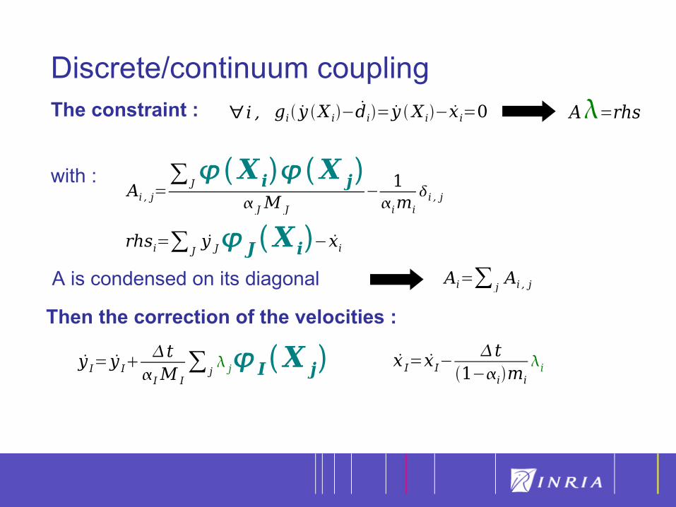
Discrete/continuum couplingThe constraint :

with :

Then the correction of the velocities :

gi y X i−di= y X i− x i=0 A=rhs∀ i ,

rhsi=∑ Jy J J X i− xi

Ai , j=∑ J

X iX j JM J

−1

imi

i , j

Ai=∑ jAi , jA is condensed on its diagonal

y I= y It

IM I∑ j

j I X j x I= xI−t

1−imi

i

14

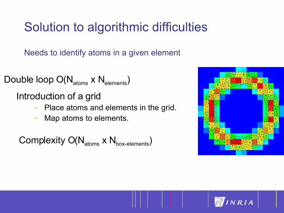
Needs to identify atoms in a given element

Solution to algorithmic difficulties

Double loop O(Natoms x Nelements)

Introduction of a grid– Place atoms and elements in the grid.– Map atoms to elements.

Complexity O(Natoms x Nbox-elements)

15

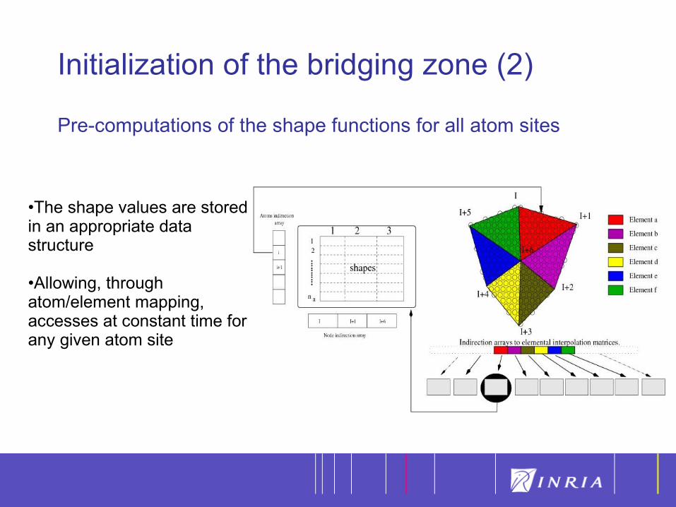
Pre-computations of the shape functions for all atom sites

Initialization of the bridging zone (2)

•The shape values are stored in an appropriate data structure

•Allowing, through atom/element mapping, accesses at constant time for any given atom site

16

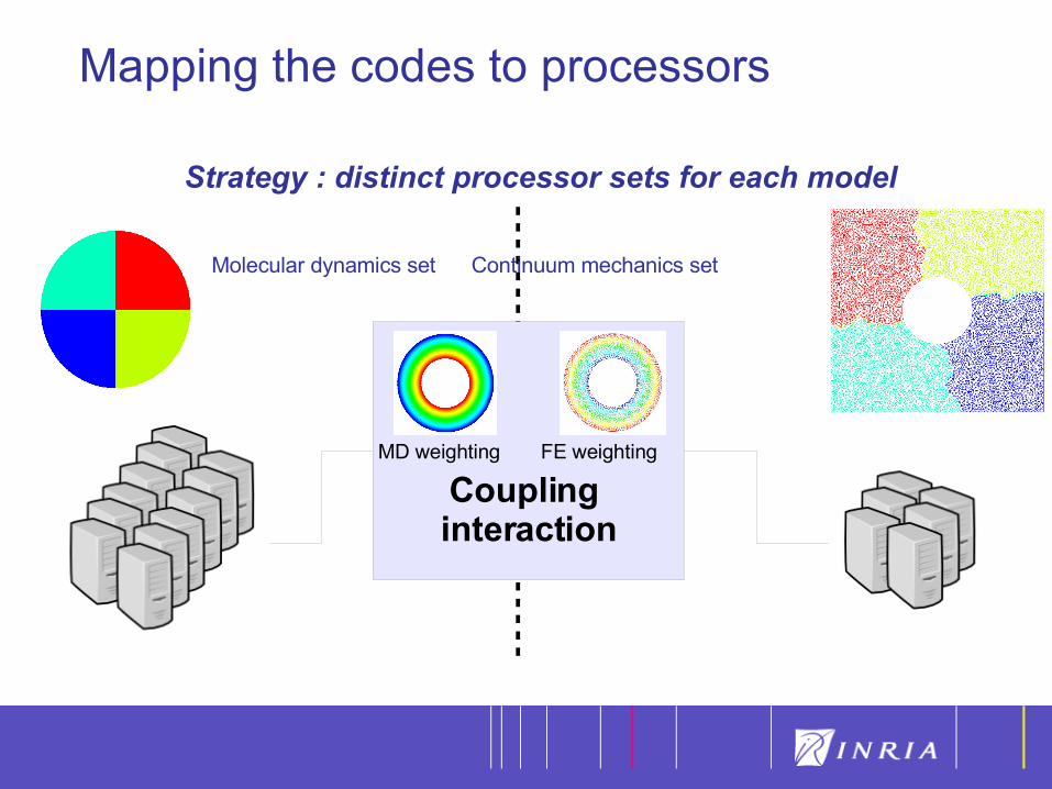
Mapping the codes to processors

Strategy : distinct processor sets for each model

Molecular dynamics set Continuum mechanics set

Coupling interaction

MD weighting FE weighting

17

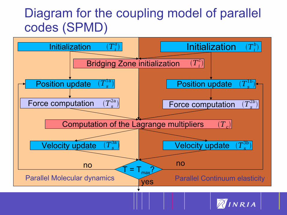
Diagram for the coupling model of parallel codes (SPMD)

Initialization

Bridging Zone initialization

Force computation

Computation of the Lagrange multipliers

Force computation

Position update Position update

T = Tmax?

Velocity update Velocity update

Initialization

no no

yesParallel Molecular dynamics Parallel Continuum elasticity

T ia T i

b

T ic

T s1bT s

1a

T s2a T s

2b

T c

T s3bT s

3a

18Details on the computation of the Lagrange Multipliers

Computation of RHS contribution

Summing the contributions

Solving the constraint system Solving the constraint system

Correcting the velocities Correcting the velocities

Computation of RHS contribution

Parallel Molecular dynamics Parallel Continuum elasticity

− xi ∑ Jy JX i

∑ J y JX i− xi=rhsi

Tc1a Tc

1b

Tc2

Tc3 Tc

3 i=rhsi/ Aii=rhsi/ Ai

Tc4a Tc

4b∑=

∆+=m

jjIj

IIM

t

1I

newI )x(yy ϕλ

α

iii m

t λα )1(

dd inewi −

∆−=

19

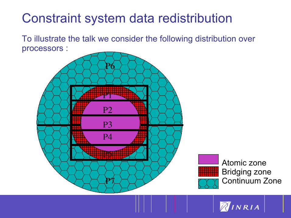
Constraint system data redistribution

To illustrate the talk we consider the following distribution over processors :

Atomic zoneBridging zoneContinuum Zone

20

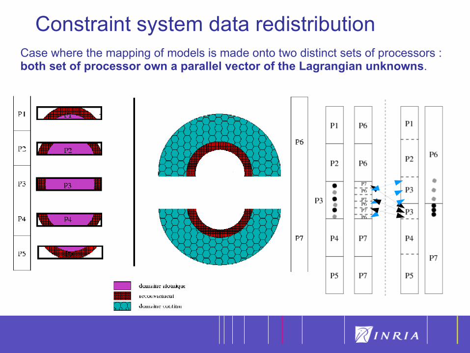
Constraint system data redistributionCase where the mapping of models is made onto two distinct sets of processors : both set of processor own a parallel vector of the Lagrangian unknowns.

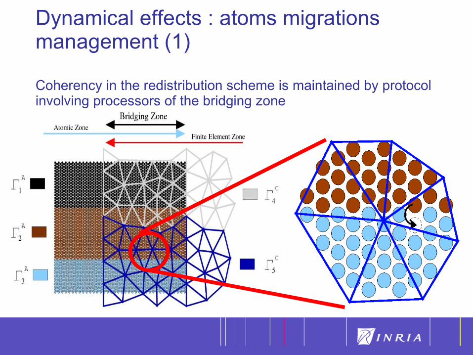
21Dynamical effects : atoms migrations management (1)

Coherency in the redistribution scheme is maintained by protocol involving processors of the bridging zone

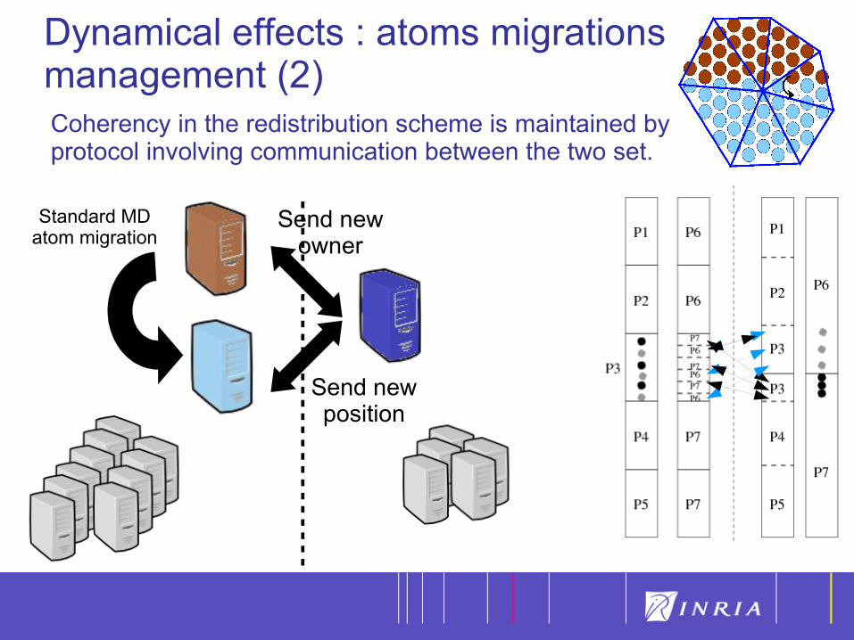
22Dynamical effects : atoms migrations management (2)Coherency in the redistribution scheme is maintained by protocol involving communication between the two set.

Send new owner

Send new position

Standard MD atom migration

23

Results

24

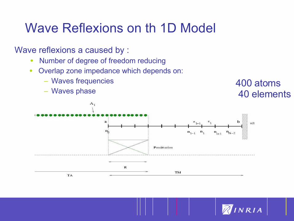
Wave Reflexions on th 1D Model

Wave reflexions a caused by :• Number of degree of freedom reducing

• Overlap zone impedance which depends on:– Waves frequencies– Waves phase

400 atoms 40 elements

25

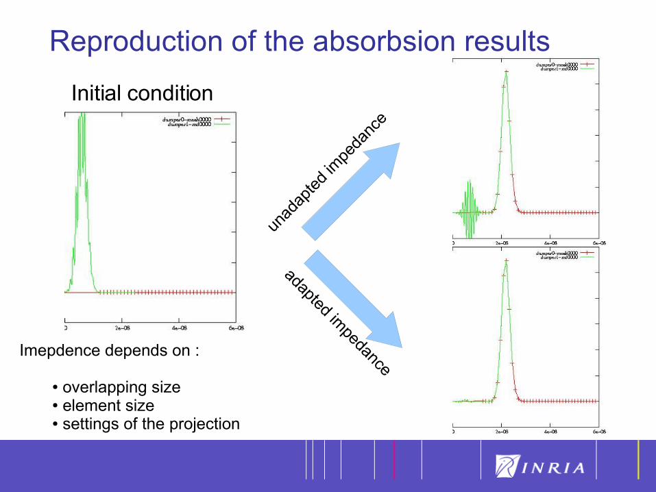
Reproduction of the absorbsion results

unad

apte

d im

peda

nce

adapted impedance

Initial condition

Imepdence depends on :

overlapping size element size settings of the projection

26

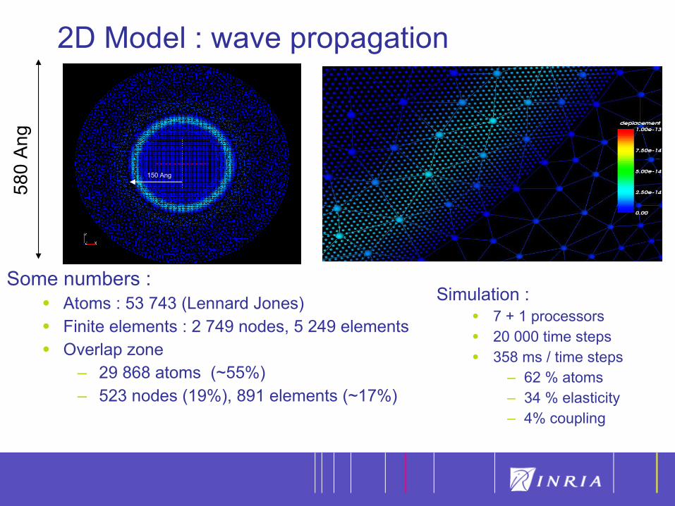
2D Model : wave propagation

Some numbers :• Atoms : 53 743 (Lennard Jones)

• Finite elements : 2 749 nodes, 5 249 elements

• Overlap zone– 29 868 atoms (~55%)– 523 nodes (19%), 891 elements (~17%)

Simulation :• 7 + 1 processors

• 20 000 time steps

• 358 ms / time steps– 62 % atoms– 34 % elasticity– 4% coupling

580

An

g

150 Ang

27

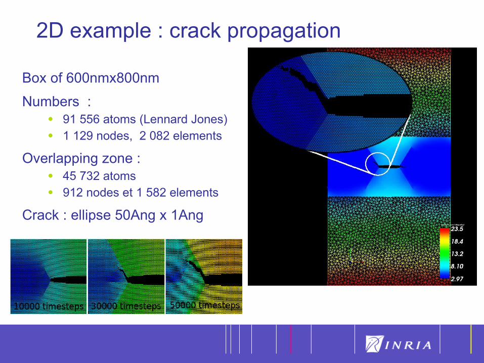
2D example : crack propagation

Box of 600nmx800nm

Numbers :• 91 556 atoms (Lennard Jones)

• 1 129 nodes, 2 082 elements

Overlapping zone : • 45 732 atoms

• 912 nodes et 1 582 elements

Crack : ellipse 50Ang x 1Ang

28

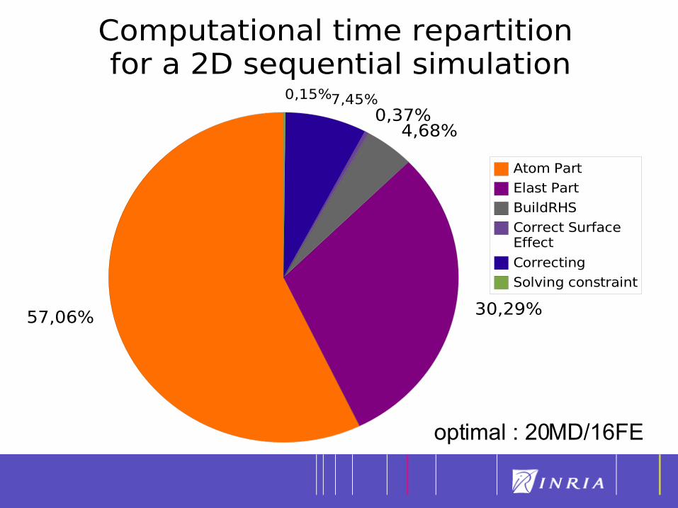
57,06% 30,29%

4,68%0,37%

7,45%0,15%

Computational time repartition for a 2D sequential simulation

Atom Part

Elast Part

BuildRHS

Correct Surface Effect

Correcting

Solving constraint

optimal : 20MD/16FE

29

4 8 16 20 24 320

0,5

1

1,5

2

2,5

3

3,5

4

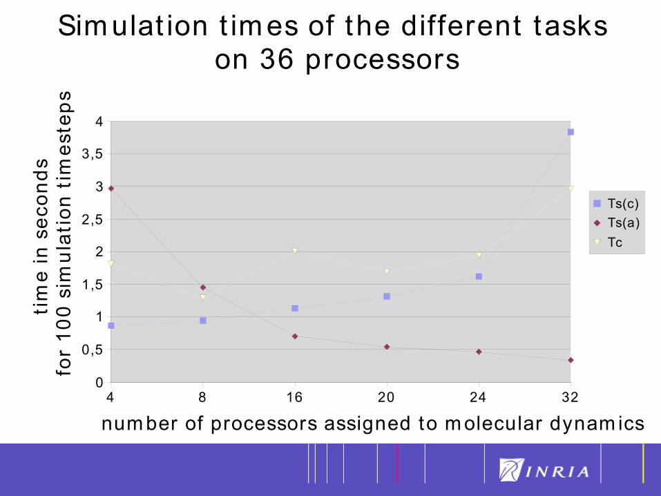
Sim ulat ion t im es of the different tasks on 36 processors

Ts(c)

Ts(a)

Tc

num ber of processors assigned to m olecular dynam ics

tim

e i

n s

eco

nd

s fo

r 1

00

sim

ula

tio

n t

ime

ste

ps

30

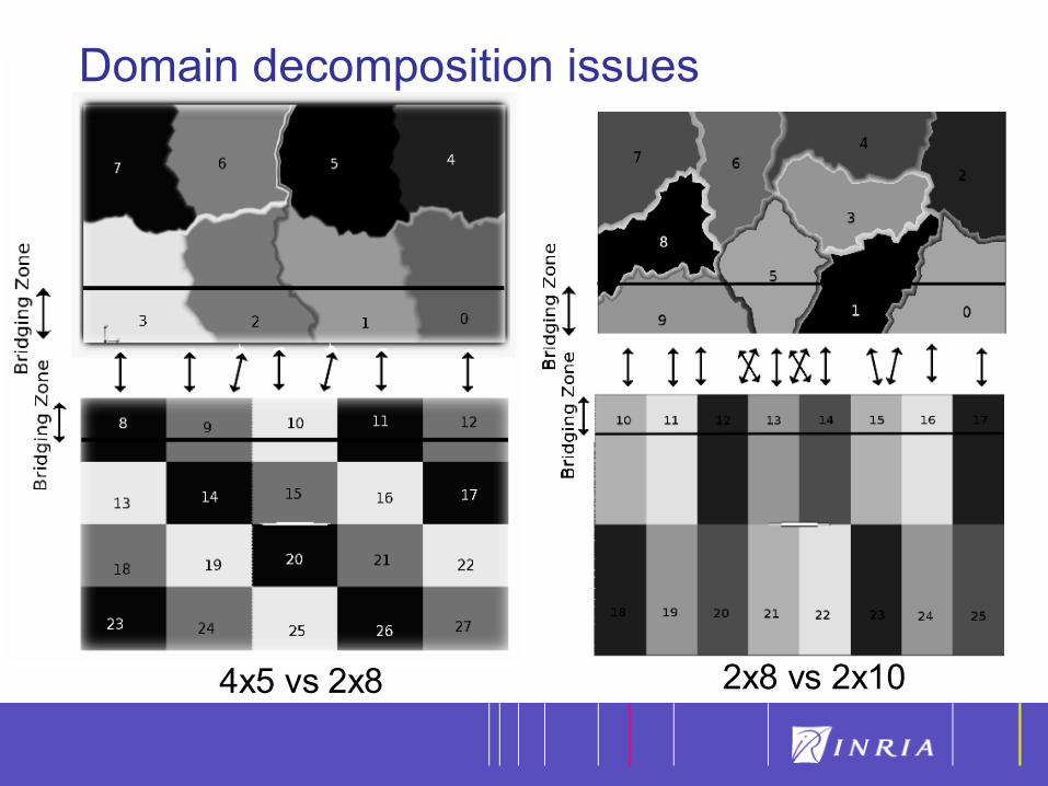
Domain decomposition issues

4x5 vs 2x8 2x8 vs 2x10

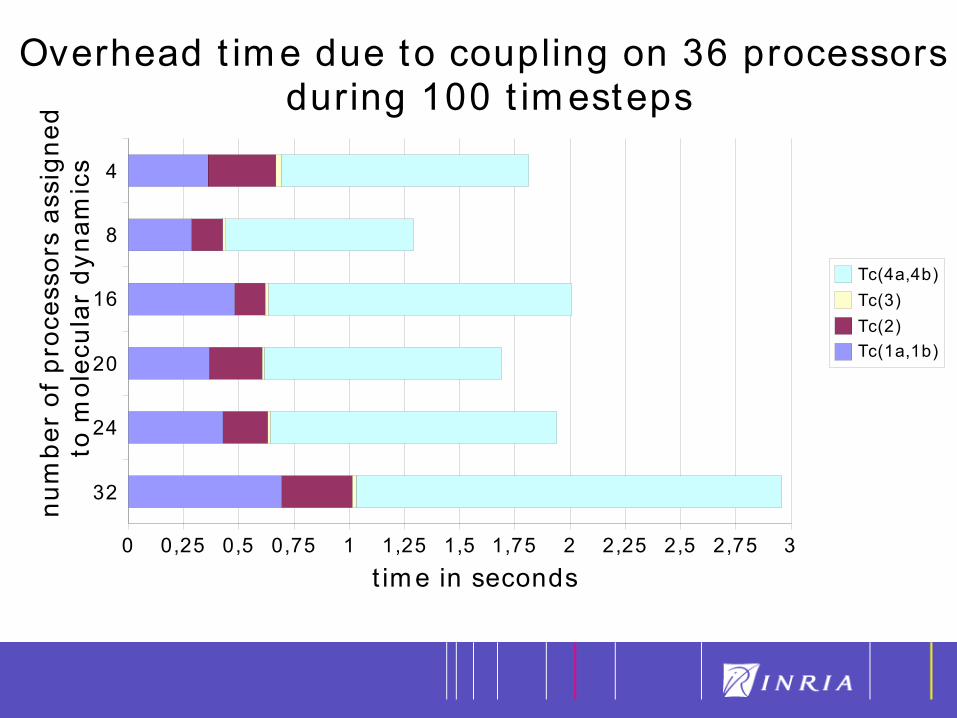
31

32

24

20

16

8

4

0 0,25 0,5 0,75 1 1,25 1,5 1,75 2 2,25 2,5 2,75 3

Overhead t im e due to coupling on 36 processors during 100 t im esteps

Tc(4a,4b)

Tc(3)

Tc(2)

Tc(1a,1b)

nu

mb

er

of

pro

cess

ors

ass

ign

ed

to

mo

lecu

lar

dy

na

mic

s

t im e in seconds

32

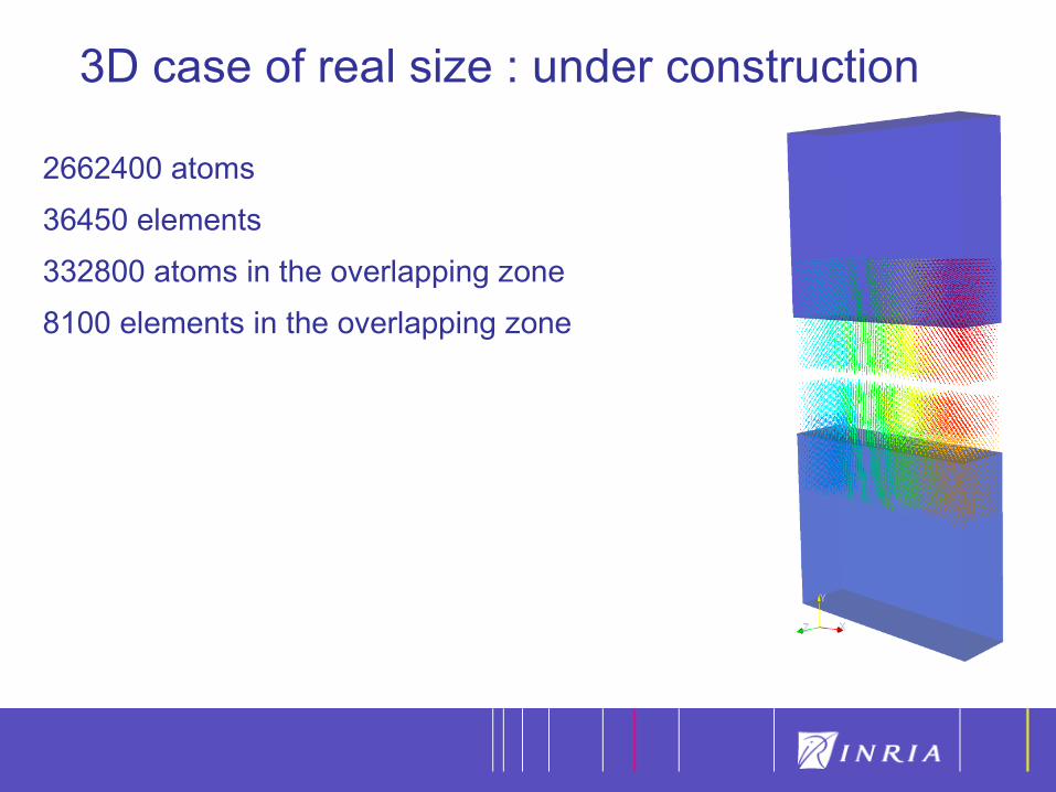
3D case of real size : under construction

2662400 atoms

36450 elements

332800 atoms in the overlapping zone

8100 elements in the overlapping zone

33

Conclusion

34

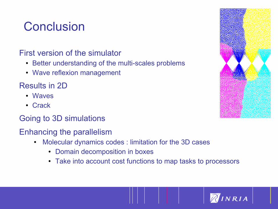
Conclusion

First version of the simulator Better understanding of the multi-scales problems Wave reflexion management

Results in 2D Waves Crack

Going to 3D simulations

Enhancing the parallelism Molecular dynamics codes : limitation for the 3D cases

Domain decomposition in boxes Take into account cost functions to map tasks to processors

35

Our simulator

T. Belytschko Model

1D, 2D and 3D tests

parallel version based on MPI communication paradigm

C++ code

Interfaced with :

finite elements : libMesh

molecular dynamics : Stamp (CEA), Lamps (Sandia)

vizualisation and steering : EPSN (ScalApplix – INRIA)