1 FINANCIAL RISK CHE 5480 Miguel Bagajewicz University of Oklahoma School of Chemical Engineering...

1

FINANCIAL RISKFINANCIAL RISK FINANCIAL RISKFINANCIAL RISK

CHE 5480CHE 5480Miguel BagajewiczMiguel Bagajewicz

University of OklahomaUniversity of OklahomaSchool of Chemical Engineering and Materials ScienceSchool of Chemical Engineering and Materials Science

CHE 5480CHE 5480Miguel BagajewiczMiguel Bagajewicz

University of OklahomaUniversity of OklahomaSchool of Chemical Engineering and Materials ScienceSchool of Chemical Engineering and Materials Science

2

Scope of DiscussionScope of DiscussionScope of DiscussionScope of Discussion

We will discuss the definition and management of financial risk in We will discuss the definition and management of financial risk in

in any design process or decision making paradigm, like…in any design process or decision making paradigm, like…

Extensions that are emerging are the treatment of other risksExtensions that are emerging are the treatment of other risks

in a multiobjective (?) framework, including for examplein a multiobjective (?) framework, including for example

• Investment PlanningInvestment Planning• Scheduling and more in general, operations planningScheduling and more in general, operations planning• Supply Chain modeling, scheduling and controlSupply Chain modeling, scheduling and control• Short term scheduling (including cash flow management)Short term scheduling (including cash flow management)• Design of process systems Design of process systems • Product DesignProduct Design

• Environmental RisksEnvironmental Risks• Accident Risks (other than those than can be expressed Accident Risks (other than those than can be expressed

as financial risk)as financial risk)

3

Introduction – Understanding RiskIntroduction – Understanding RiskIntroduction – Understanding RiskIntroduction – Understanding Risk

Profit Histogram

0.00

0.05

0.10

0.15

0.20

0.25

0.30

0.35

0.40

0.45

-300 -200 -100 0 100 200 300 400 500 600 700 800

Profit (M$)

Probability

Investment Plan I - E[Profit ] = 338

Investment Plan II - E[Profit ] = 335

Probability of Loss

for Plan I = 12%

Consider two investment plans, designs, or operational decisionsConsider two investment plans, designs, or operational decisions

4

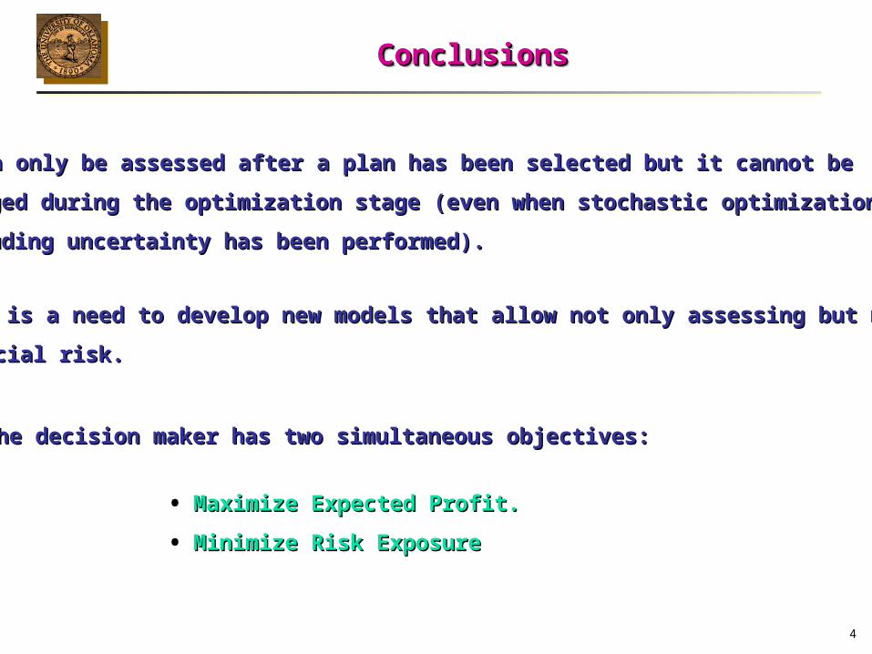
ConclusionsConclusionsConclusionsConclusions

Risk can only be assessed after a plan has been selected but it cannot be Risk can only be assessed after a plan has been selected but it cannot be

managed during the optimization stage (even when stochastic optimization managed during the optimization stage (even when stochastic optimization

including uncertainty has been performed). including uncertainty has been performed).

The decision maker has two simultaneous objectives:The decision maker has two simultaneous objectives:

There is a need to develop new models that allow not only assessing but managingThere is a need to develop new models that allow not only assessing but managing

financial risk. financial risk.

• Maximize Expected Profit. Maximize Expected Profit.

• Minimize Risk ExposureMinimize Risk Exposure

5

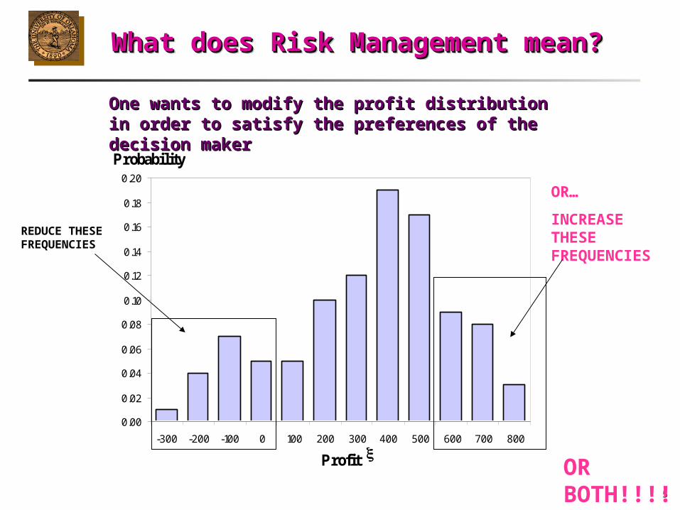
What does Risk Management mean?What does Risk Management mean?What does Risk Management mean?What does Risk Management mean?

0.00

0.02

0.04

0.06

0.08

0.10

0.12

0.14

0.16

0.18

0.20

-300 -200 -100 0 100 200 300 400 500 600 700 800

Profit x

Probability

REDUCE THESE FREQUENCIES

OR…

INCREASE THESE FREQUENCIES

One wants to modify the profit distribution in order to satisfy One wants to modify the profit distribution in order to satisfy the preferences of the decision makerthe preferences of the decision maker

OR BOTH!!!!

6

Characteristics of Two-StageCharacteristics of Two-StageStochastic Optimization Models Stochastic Optimization Models


PhilosophyPhilosophy• Maximize the Maximize the Expected ValueExpected Value of the objective over all possible realizations of of the objective over all possible realizations of

uncertain parameters.uncertain parameters.• Typically, the objective is Typically, the objective is Expected ProfitExpected Profit , usually , usually Net Present ValueNet Present Value..• Sometimes the minimization of Sometimes the minimization of CostCost is an alternative objective. is an alternative objective.

UncertaintyUncertainty• Typically, the uncertain parameters are: Typically, the uncertain parameters are: market demands, availabilities,market demands, availabilities,

prices, process yields, rate of interest, inflation, etc.prices, process yields, rate of interest, inflation, etc.• In Two-Stage Programming, uncertainty is modeled through a finite numberIn Two-Stage Programming, uncertainty is modeled through a finite number

of independent of independent ScenariosScenarios..• Scenarios are typically formed by Scenarios are typically formed by random samplesrandom samples taken from the probability taken from the probability

distributions of the uncertain parameters.distributions of the uncertain parameters.

7

First-Stage DecisionsFirst-Stage Decisions• Taken before the uncertainty is revealed. They usually correspond to structural Taken before the uncertainty is revealed. They usually correspond to structural

decisions (not operational). decisions (not operational). • Also called “Here and Now” decisions.Also called “Here and Now” decisions.• Represented by “Design” Variables.Represented by “Design” Variables.• Examples:Examples:



−To build a plant or not. How much capacity should be added, etc. To build a plant or not. How much capacity should be added, etc. −To place an order now. To place an order now. −To sign contracts or buy options. To sign contracts or buy options. −To pick a reactor volume, to pick a certain number of trays and size To pick a reactor volume, to pick a certain number of trays and size

the condenser and the reboiler of a column, etc the condenser and the reboiler of a column, etc

8

Second-Stage DecisionsSecond-Stage Decisions• Taken in order to adapt the plan or design to the uncertain parameters Taken in order to adapt the plan or design to the uncertain parameters

realization.realization.• Also called “Recourse” decisions.Also called “Recourse” decisions.• Represented by “Control” Variables.Represented by “Control” Variables.• Example: the operating level; the production slate of a plant.Example: the operating level; the production slate of a plant.

• Sometimes first stage decisions can be treated as second stage decisions. Sometimes first stage decisions can be treated as second stage decisions.

In such case the problem is called a multiple stage problem. In such case the problem is called a multiple stage problem.

ShortcomingsShortcomings• The model is unable to perform risk management decisions.The model is unable to perform risk management decisions.



9

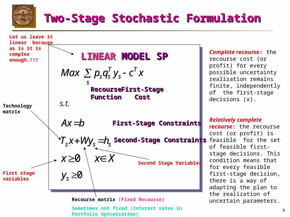
Two-Stage Stochastic FormulationTwo-Stage Stochastic FormulationTwo-Stage Stochastic FormulationTwo-Stage Stochastic Formulation

LINEAR LINEAR MODEL SPMODEL SPLINEAR LINEAR MODEL SPMODEL SP

xcyqpMax T

ss

Tss xcyqpMax T

ss

Tss

bAxbAx

Xxx 0 Xxx 0

sss hWyxT sss hWyxT

0sy 0sy

s.t.s.t.

First-Stage ConstraintsFirst-Stage Constraints

Second-Stage ConstraintsSecond-Stage Constraints

RecourseRecourseFunctionFunction

First-StageFirst-StageCostCost

First stage variables

Second Stage Variables

Technology matrix

Recourse matrix (Fixed Recourse)

Sometimes not fixed (Interest rates in Portfolio Optimization)

Complete recourse: the recourse cost (or profit) for every possible uncertainty realization remains finite, independently of the first-stage decisions (x).

Relatively complete recourse: the recourse cost (or profit) is feasible for the set of feasible first-stage decisions. This condition means that for every feasible first-stage decision, there is a way of adapting the plan to the realization of uncertain parameters.

We also have found that one can sacrifice efficiency for certain scenarios to improve risk management. We do not know how to call this yet.

Let us leave it linear because as is it is complex enough.!!!

10

Robust Optimization Using Variance (Robust Optimization Using Variance (Mulvey et al., 1995)Mulvey et al., 1995)

Previous Approaches to Risk ManagementPrevious Approaches to Risk ManagementPrevious Approaches to Risk ManagementPrevious Approaches to Risk Management

0.0

0.1

0.2

0.3

0.4

0.5

0.6

0.7

0.8

0.9

-2.5 -2.0 -1.5 -1.0 -0.5 0.0 0.5 1.0 1.5 2.0 2.5 3.0 3.5 4.0 4.5 5.0 5.5

Profit

Profit PDF Expected Profit

Variance is a measurefor the dispersionof the distribution

Desirable Penalty

Maximize E[Profit] - Maximize E[Profit] - ·V[Profit]·V[Profit]

Underlying Assumption: Underlying Assumption: Risk is monotonic with variabilityRisk is monotonic with variability

Undesirable Penalty

11

Robust Optimization Using VarianceRobust Optimization Using VarianceRobust Optimization Using VarianceRobust Optimization Using Variance

DrawbacksDrawbacks

• Variance is a symmetric risk measure: profits both above and below the targetVariance is a symmetric risk measure: profits both above and below the target

level are penalized equally. We only want to penalize profits below the target.level are penalized equally. We only want to penalize profits below the target.

• Introduces non-linearities in the model, which results in serious computationalIntroduces non-linearities in the model, which results in serious computational

difficulties, specially difficulties, specially in large-scale problems.in large-scale problems.

• The model may render solutions that are stochastically dominated by others.The model may render solutions that are stochastically dominated by others.

This is known in the literature as not showing Pareto-Optimality. In other wordsThis is known in the literature as not showing Pareto-Optimality. In other words

there is a better solution (ythere is a better solution (yss,x,x**) than the one obtained ) than the one obtained (y(yss**,x*). ,x*).

12

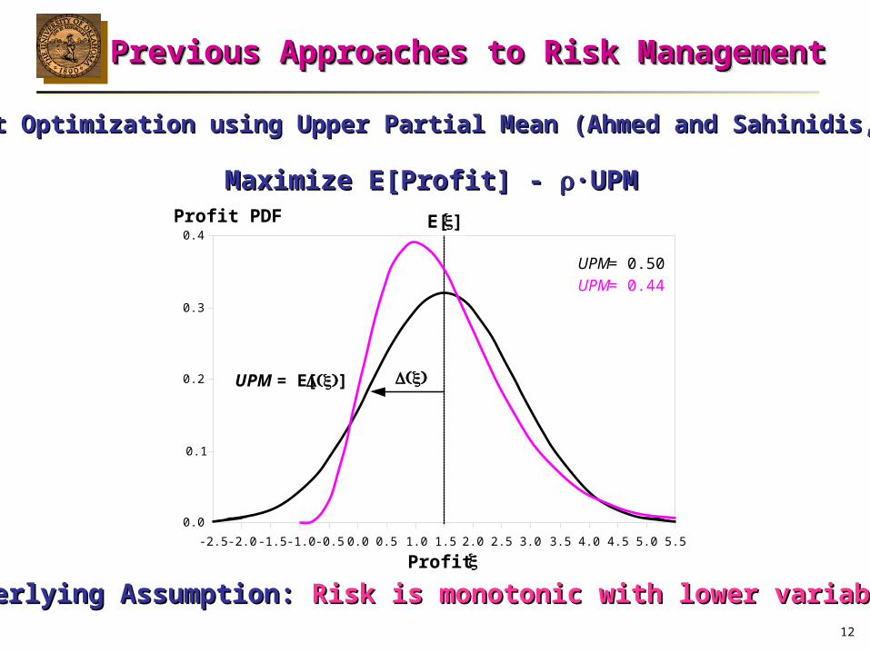
Robust Optimization using Upper Partial Mean (Ahmed and Sahinidis, 1998)Robust Optimization using Upper Partial Mean (Ahmed and Sahinidis, 1998)


x

0.0

0.1

0.2

0.3

0.4

-2.5 -2.0 -1.5 -1.0 -0.5 0.0 0.5 1.0 1.5 2.0 2.5 3.0 3.5 4.0 4.5 5.0 5.5

Profit x

Profit PDF

UPM = E[x ]

E[x ]

UPM = 0.50

UPM = 0.44

Maximize E[Profit] - Maximize E[Profit] - ·UPM·UPM

Underlying Assumption: Underlying Assumption: Risk is monotonic with lower variabilityRisk is monotonic with lower variability

13

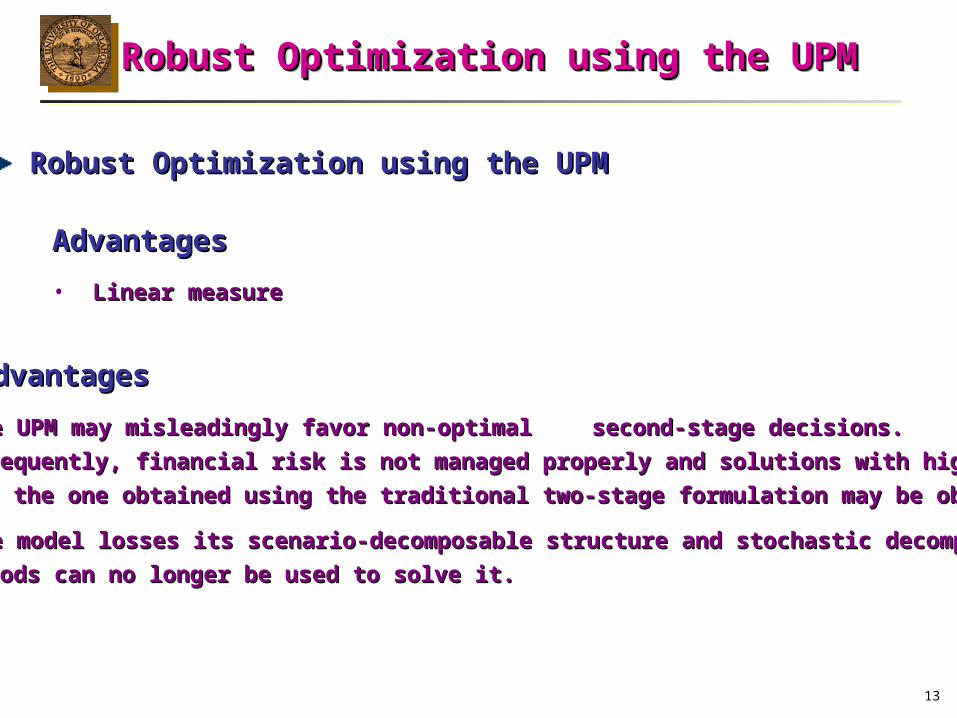
Robust Optimization using the UPMRobust Optimization using the UPMRobust Optimization using the UPMRobust Optimization using the UPM

AdvantagesAdvantages

• Linear measureLinear measure

Robust Optimization using the UPMRobust Optimization using the UPM

DisadvantagesDisadvantages

• The UPM may misleadingly favor non-optimalThe UPM may misleadingly favor non-optimal second-stage decisions.second-stage decisions.

• Consequently, financial risk is not managed properly and solutions with higher riskConsequently, financial risk is not managed properly and solutions with higher risk

than the one obtained using the traditional two-stage formulation may be obtained.than the one obtained using the traditional two-stage formulation may be obtained.

• The model losses its scenario-decomposable structure and stochastic decompositionThe model losses its scenario-decomposable structure and stochastic decomposition

methods can no longer be used to solve it.methods can no longer be used to solve it.

14


s

Skkks ProfitProfitpMax ; 0

= 3= 3Profits s

Case I Case II Case I Case II

S1 150 100 0 0

S2 125 100 0 0

S3 75 75 25 6.25

S4 50 50 50 31.25

E[Profit] 100.00 81.25

UPM 18.75 9.38

Objective 43.75 53.13

Ss

sspUPM

Objective Function: Maximize E[Profit] - Objective Function: Maximize E[Profit] - ·UPM·UPM

Downside scenarios are the same, but the UPM is affected by Downside scenarios are the same, but the UPM is affected by the change in expected profit due to a different upside distribution. the change in expected profit due to a different upside distribution. As a result a wrong choice is made. As a result a wrong choice is made.

15

Effect of Non-Optimal Second-Stage DecisionsEffect of Non-Optimal Second-Stage Decisions


P1 A

P2 B

P1 A

P2 B

P1 A

P2 B

-380

-360

-340

-320

-300

-280

-260

-240

-220

-200

0 20 40 60 80 100 120 140 160 180 200 220

E[Profit ]

Robustness Solution

Robustness Solution with Optimal Second-Stage Decisions

0

2

4

6

8

10

12

14

16

18

0 20 40 60 80 100 120 140 160 180 200 220

UPM

Robustness Solution


Both technologies are able to produce two products with different production cost and at different yield per unit of installed capacity

-380

-360

-340

-320

-300

-280

-260

-240

-220

-200

0 1 2 3 4 5 6 7 8 9 10 11 12 13 14 15 16 17

UPM

E[Profit ]

Robustness Solution


16

OTHER APPROACHESOTHER APPROACHESOTHER APPROACHESOTHER APPROACHES

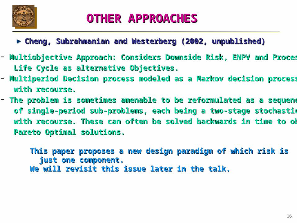
Cheng, Subrahmanian and Westerberg (2002, unpublished)Cheng, Subrahmanian and Westerberg (2002, unpublished)Cheng, Subrahmanian and Westerberg (2002, unpublished)Cheng, Subrahmanian and Westerberg (2002, unpublished)

This paper proposes a new design paradigm of which risk is just one component. This paper proposes a new design paradigm of which risk is just one component. We will revisit this issue later in the talk.We will revisit this issue later in the talk.

− Multiobjective Approach: Considers Downside Risk, ENPV and Process Multiobjective Approach: Considers Downside Risk, ENPV and Process

Life Cycle as alternative Objectives.Life Cycle as alternative Objectives.− Multiperiod Decision process modeled as a Markov decision process Multiperiod Decision process modeled as a Markov decision process

with recourse.with recourse.− The problem is sometimes amenable to be reformulated as a sequence The problem is sometimes amenable to be reformulated as a sequence

of single-period sub-problems, each being a two-stage stochastic program of single-period sub-problems, each being a two-stage stochastic program

with recourse. These can often be solved backwards in time to obtain with recourse. These can often be solved backwards in time to obtain

Pareto Optimal solutions. Pareto Optimal solutions.

17

OTHER APPROACHESOTHER APPROACHESOTHER APPROACHESOTHER APPROACHES

Risk Premium (Applequist, Pekny and Reklaitis, 2000)Risk Premium (Applequist, Pekny and Reklaitis, 2000)

− Observation: Rate of return varies linearly with variability. The Observation: Rate of return varies linearly with variability. The

of such dependance is called Risk Premium. of such dependance is called Risk Premium. − They suggest to benchmark new investments against the historical They suggest to benchmark new investments against the historical − risk premium by using a two objective (risk premium and profit) risk premium by using a two objective (risk premium and profit) − problem. problem. −The technique relies on using variance as a measure of variability.The technique relies on using variance as a measure of variability.

18

ConclusionsConclusions

• The minimization of Variance penalizes both sides of the mean. The minimization of Variance penalizes both sides of the mean.

• The Robust Optimization Approach using Variance or UPM is not suitable The Robust Optimization Approach using Variance or UPM is not suitable

for risk management.for risk management.

• The Risk Premium Approach (Applequist et al.) has the same problems The Risk Premium Approach (Applequist et al.) has the same problems

as the penalization of variance.as the penalization of variance.

THUS, THUS,

• Risk should be properly defined and Risk should be properly defined and directly directly incorporated in the models to incorporated in the models to

manage it. manage it.

• The multiobjective Markov decision process (Applequist et al, 2000) The multiobjective Markov decision process (Applequist et al, 2000)

is very closely related to ours and can be considered complementary. In is very closely related to ours and can be considered complementary. In

fact (Westerberg dixit) it can be extended to match ours in the definition fact (Westerberg dixit) it can be extended to match ours in the definition

of risk and its multilevel parametrization. of risk and its multilevel parametrization.


19

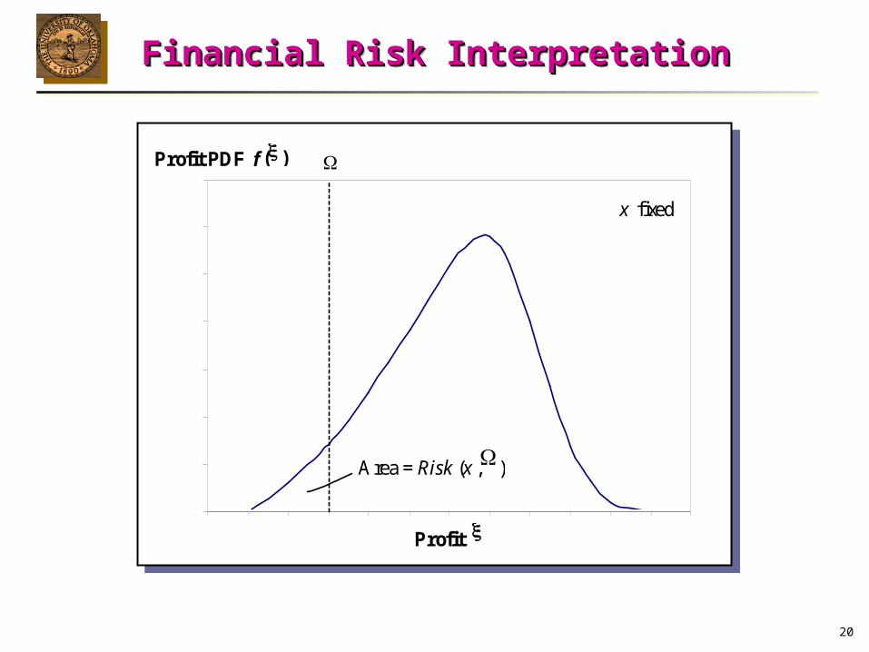
Financial Risk = Probability that a plan or Financial Risk = Probability that a plan or design does not meet a certain profit targetdesign does not meet a certain profit targetFinancial Risk = Probability that a plan or Financial Risk = Probability that a plan or design does not meet a certain profit targetdesign does not meet a certain profit target

Probabilistic Definition of RiskProbabilistic Definition of Risk Probabilistic Definition of RiskProbabilistic Definition of Risk

zzss is a new is a new binarybinary variable variablezzss is a new is a new binarybinary variable variable

Formal Definition of Financial RiskFormal Definition of Financial RiskFormal Definition of Financial RiskFormal Definition of Financial Risk

ProfitPxRisk ),( ProfitPxRisk ),(

Scenarios are independent eventsScenarios are independent eventsScenarios are independent eventsScenarios are independent events s

ss ProfitPpxRisk ),( s

ss ProfitPpxRisk ),(

else0

If1 ss

ProfitProfitP

else0

If1 ss

ProfitProfitP

ss zProfitP ss zProfitP

s

ss zpxRisk ),( s

ss zpxRisk ),(

For each scenario the profit is eitherFor each scenario the profit is eithergreater/equal or smaller than the targetgreater/equal or smaller than the targetFor each scenario the profit is eitherFor each scenario the profit is eithergreater/equal or smaller than the targetgreater/equal or smaller than the target

20

Financial Risk InterpretationFinancial Risk InterpretationFinancial Risk InterpretationFinancial Risk Interpretation

0.00

0.02

0.04

0.06

0.08

0.10

0.12

0.14

0.16

0.18

0.20

Profit x

Probability

Cumulative Probability = Risk (x ,)

0.00

0.02

0.04

0.06

0.08

0.10

0.12

0.14

Profit x

Area = Risk (x ,)

x fixed

Profit PDF f (x )

21

Cumulative Risk CurveCumulative Risk CurveCumulative Risk CurveCumulative Risk Curve

Our intention is to modify the shape and location of thiscurve according to the attitude towards risk of the decision makerOur intention is to modify the shape and location of thiscurve according to the attitude towards risk of the decision maker

0.0

0.1

0.2

0.3

0.4

0.5

0.6

0.7

0.8

0.9

1.0

250 500 750 1000 1250 1500 1750 2000 2250 2500 2750 3000 3250

Profit (M$)

Risk

22

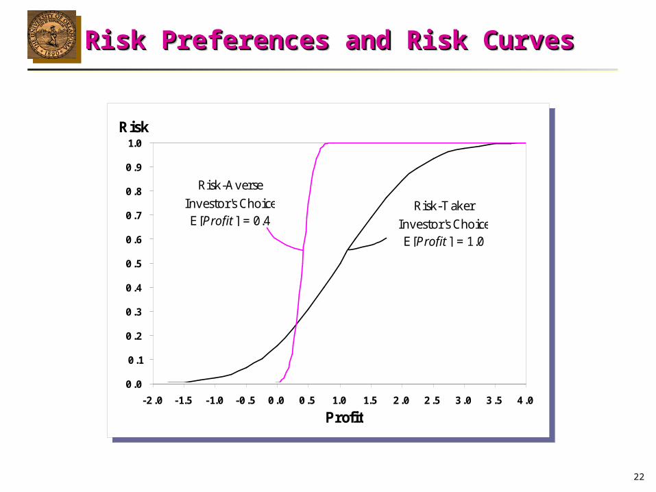
Risk Preferences and Risk CurvesRisk Preferences and Risk CurvesRisk Preferences and Risk CurvesRisk Preferences and Risk Curves

0.0

0.1

0.2

0.3

0.4

0.5

0.6

0.7

0.8

0.9

1.0

-2.0 -1.5 -1.0 -0.5 0.0 0.5 1.0 1.5 2.0 2.5 3.0 3.5 4.0

Profit

Risk

Risk-Averse

Investor's ChoiceE[Profit ] = 0.4

Risk-T aker

Investor's ChoiceE[Profit ] = 1.0

23

Risk Curve PropertiesRisk Curve PropertiesRisk Curve PropertiesRisk Curve Properties

A plan or design with Maximum E[A plan or design with Maximum E[ProfitProfit] (i.e. optimal in Model SP) sets a ] (i.e. optimal in Model SP) sets a

theoretical limit for financial risk: it is impossible to find a feasible plan/design theoretical limit for financial risk: it is impossible to find a feasible plan/design

having a risk curve entirely beneath this curve.having a risk curve entirely beneath this curve.

A plan or design with Maximum E[A plan or design with Maximum E[ProfitProfit] (i.e. optimal in Model SP) sets a ] (i.e. optimal in Model SP) sets a

theoretical limit for financial risk: it is impossible to find a feasible plan/design theoretical limit for financial risk: it is impossible to find a feasible plan/design

having a risk curve entirely beneath this curve.having a risk curve entirely beneath this curve.

0.0

0.1

0.2

0.3

0.4

0.5

0.6

0.7

0.8

0.9

1.0

Profit

Risk

Maximum

E[Profit ]

Impossible

curve

Possible

curve

24

Minimizing Risk: a Multi-Objective ProblemMinimizing Risk: a Multi-Objective ProblemMinimizing Risk: a Multi-Objective ProblemMinimizing Risk: a Multi-Objective Problem

)1,0(

)1(

s

ssT

sTs

ssT

sTs

z

zUxcyq

zUxcyq

Xxx 0

0sy

s.t.

xcyqp ProfitMax E T

ssss

s

ss zp Min Risk 11

s

sisi zp Min Risk

...

bAx

sss hWyxT

Multiple Objectives:Multiple Objectives:• At each profit we want minimize the associated riskAt each profit we want minimize the associated risk• We also want to maximize the expected profitWe also want to maximize the expected profit

0.0

0.1

0.2

0.3

0.4

0.5

0.6

0.7

0.8

0.9

1.0

Target Profit

Risk

x fixed

1 2 3 4

Min Risk (x ,1)

Min Risk (x ,2)

Min Risk (x ,3)

Min Risk (x ,4)

Max E[Profit (x )]

25

Restricted RiskRestricted Risk MODELMODELRestricted RiskRestricted Risk MODELMODEL

Risk ManagementRisk ManagementConstraintsConstraints


xcyqpMax T

ssss

s.t.

is

sis εzp

)1,0(

)1(

s

sisiT

sTs

sisiT

sTs

z

zUxcyq

zUxcyq

Xxx 0

0sy

bAx

sss hWyxT

Forces Risk to be lowerForces Risk to be lowerthan a specified levelthan a specified level

Parametric Representations of theParametric Representations of the Multi-Objective Model – Restricted RiskMulti-Objective Model – Restricted Risk

Parametric Representations of theParametric Representations of the Multi-Objective Model – Restricted RiskMulti-Objective Model – Restricted Risk

26

Parametric Representations of theParametric Representations of the Multi-Objective Model – Penalty for RiskMulti-Objective Model – Penalty for Risk

Parametric Representations of theParametric Representations of the Multi-Objective Model – Penalty for RiskMulti-Objective Model – Penalty for Risk

s.t.

i s

sisiT

ss

Tss zpxc yqpMax

Penalty TermPenalty TermPenalty TermPenalty Term

Risk PenaltyRisk Penalty MODELMODELRisk PenaltyRisk Penalty MODELMODEL



)1,0(

)1(

s

sisiT

sTs

sisiT

sTs

z

zUxcyq

zUxcyq

Xxx 0

0sy

bAx

sss hWyxT

Define several profit Define several profit

Targets and penaltyTargets and penalty

weights to solve theweights to solve the

model using a multi-model using a multi-

parametric approachparametric approach

STRATEGYSTRATEGYSTRATEGYSTRATEGY

27


• Risk can be effectively managed according to the decision maker’s criteria.Risk can be effectively managed according to the decision maker’s criteria.

• The models can adapt to risk-averse or risk-taker decision makers, and theirThe models can adapt to risk-averse or risk-taker decision makers, and their

risk preferences are easily matched using the risk curves.risk preferences are easily matched using the risk curves.

• A full spectrum of solutions is obtained. These solutions always haveA full spectrum of solutions is obtained. These solutions always have

optimal second-stage decisions.optimal second-stage decisions.

• Model Risk Penalty conserves all the properties of the standard two-stageModel Risk Penalty conserves all the properties of the standard two-stage

stochastic formulation.stochastic formulation.

Risk Management using the New ModelsRisk Management using the New ModelsRisk Management using the New ModelsRisk Management using the New Models

DisadvantagesDisadvantages

• The use of binary variables is required, which increases the computational The use of binary variables is required, which increases the computational

time to get a solution. This is a major limitation for large-scale problems.time to get a solution. This is a major limitation for large-scale problems.

28

Computational IssuesComputational Issues

Risk Management using the New ModelsRisk Management using the New ModelsRisk Management using the New ModelsRisk Management using the New Models

• The most efficient methods to solve stochastic optimization problems reportedThe most efficient methods to solve stochastic optimization problems reported

in the literature exploit the decomposable structure of the model. in the literature exploit the decomposable structure of the model.

• This property means that each scenario defines an independent second-stageThis property means that each scenario defines an independent second-stage

problem that can be solved separately from the other scenarios once the first-problem that can be solved separately from the other scenarios once the first-

stage variables are fixed.stage variables are fixed.

• The Risk Penalty Model is decomposable whereas Model Restricted Risk is not.The Risk Penalty Model is decomposable whereas Model Restricted Risk is not.

Thus, the first one is model is preferable.Thus, the first one is model is preferable.

• Even using decomposition methods, the presence of binary variables in bothEven using decomposition methods, the presence of binary variables in both

models constitutes a major computational limitation to solve large-scale problems.models constitutes a major computational limitation to solve large-scale problems.

• It would be more convenient to measure risk indirectly such that binary variablesIt would be more convenient to measure risk indirectly such that binary variables

in the second stage are avoided.in the second stage are avoided.

29

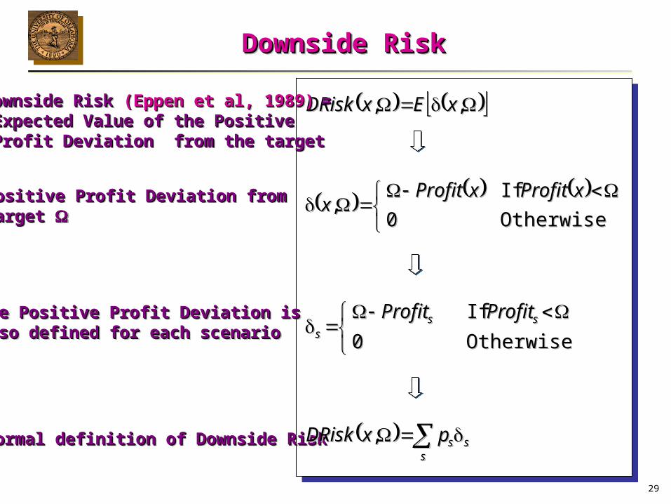
,, xExDRisk ,, xExDRiskDownside Risk Downside Risk (Eppen et al, 1989)(Eppen et al, 1989) == Expected Value of the PositiveExpected Value of the Positive Profit Deviation from the targetProfit Deviation from the target

Downside Risk Downside Risk (Eppen et al, 1989)(Eppen et al, 1989) == Expected Value of the PositiveExpected Value of the Positive Profit Deviation from the targetProfit Deviation from the target

Downside RiskDownside Risk Downside RiskDownside Risk

Positive Profit Deviation fromPositive Profit Deviation fromTarget Target Positive Profit Deviation fromPositive Profit Deviation fromTarget Target

Formal definition of Downside RiskFormal definition of Downside RiskFormal definition of Downside RiskFormal definition of Downside Risk

Otherwise0

If,

xProfitxProfitx

Otherwise0

If,

xProfitxProfitx

s

sspxDRisk , s

sspxDRisk ,

The Positive Profit Deviation isThe Positive Profit Deviation isalso defined for each scenarioalso defined for each scenarioThe Positive Profit Deviation isThe Positive Profit Deviation isalso defined for each scenarioalso defined for each scenario

Otherwise0

If sss

ProfitProfit

Otherwise0

If sss

ProfitProfit

30

Downside Risk InterpretationDownside Risk InterpretationDownside Risk InterpretationDownside Risk Interpretation

0.00

0.02

0.04

0.06

0.08

0.10

0.12

0.14

Profit x

x fixed

DRisk (x ,) = E[(x ,)]

Profit PDF f (x )

ò

¥xxx dfxDRisk )(),(

31

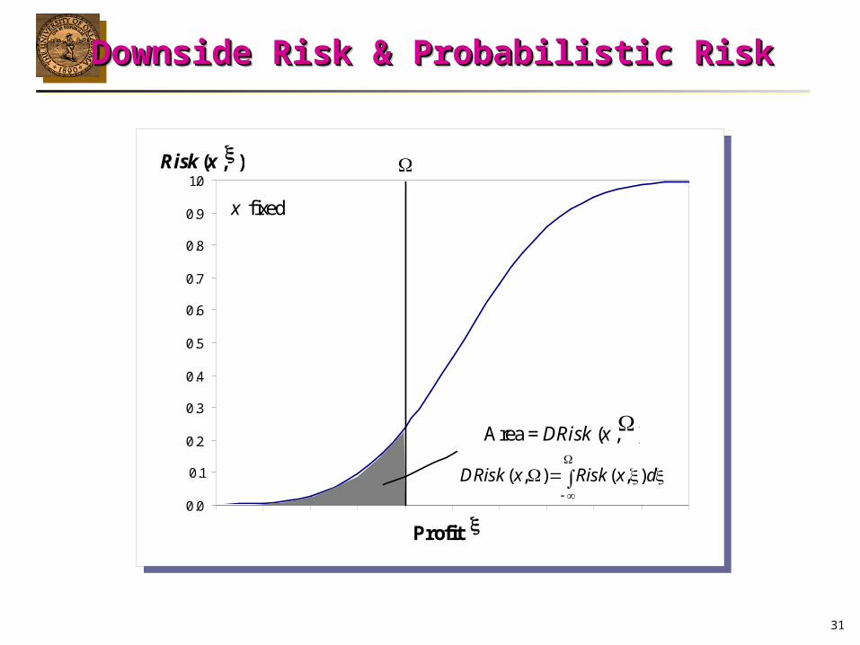
Downside Risk & Probabilistic RiskDownside Risk & Probabilistic RiskDownside Risk & Probabilistic RiskDownside Risk & Probabilistic Risk

0.0

0.1

0.2

0.3

0.4

0.5

0.6

0.7

0.8

0.9

1.0

Profit x

Risk (x ,x )

x fixed

Area = DRisk (x ,)

ò

¥xx dxRiskxDRisk ),(),(

32

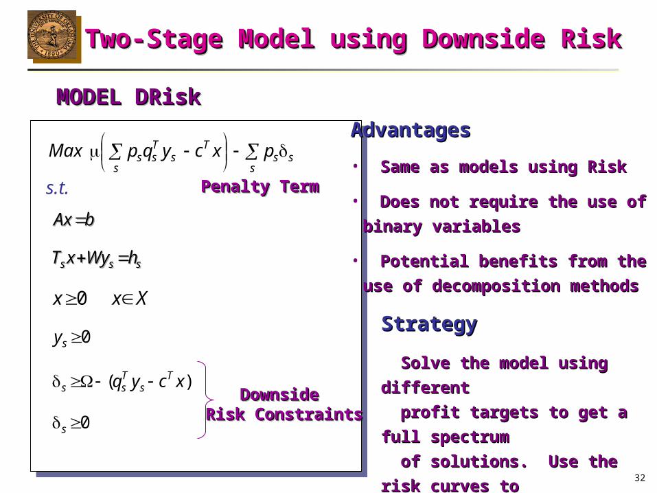
Two-Stage Model using Downside RiskTwo-Stage Model using Downside RiskTwo-Stage Model using Downside RiskTwo-Stage Model using Downside Risk

s.t.

sss

T

ss

Tss pxc yqpMax

Penalty TermPenalty TermPenalty TermPenalty Term

MODEL DRiskMODEL DRiskMODEL DRiskMODEL DRisk

Downside Downside Risk ConstraintsRisk Constraints

Downside Downside Risk ConstraintsRisk Constraints

)( xcyq Ts

Tss

Xxx 0

0sy

bAxbAx

sss hWyxT sss hWyxT

0s


• Same as models using RiskSame as models using Risk

• Does not require the use ofDoes not require the use of

binary variablesbinary variables

• Potential benefits from thePotential benefits from the

use of decomposition methodsuse of decomposition methods

StrategyStrategy

Solve the model using differentSolve the model using different

profit targets to get a full spectrumprofit targets to get a full spectrum

of solutions. Use the risk curves toof solutions. Use the risk curves to

select the solution that better suitsselect the solution that better suits

the decision maker’s preferencethe decision maker’s preference

33

Two-Stage Model using Downside RiskTwo-Stage Model using Downside RiskTwo-Stage Model using Downside RiskTwo-Stage Model using Downside Risk

Warning: Warning: The same risk may imply different Downside Risks. The same risk may imply different Downside Risks.

0.0

0.1

0.2

0.3

0.4

0.5

0.6

0.7

0.8

0.9

1.0

-2.0 -1.5 -1.0 -0.5 0.0 0.5 1.0 1.5 2.0 2.5 3.0 3.5 4.0

Profit

Risk

DRisk (Design I , 0.5) = 0.2

Risk (Design I , 0.5) = 0.5

DRisk (Design II , 0.5) = 0.2

Risk (Design II , 0.5) = 0.309

Immediate Consequence: Immediate Consequence:

Minimizing downside risk does not guarantee minimizing risk.Minimizing downside risk does not guarantee minimizing risk.

34

Riskoptimizer (Palisades) and CrystalBall (Decisioneering)Riskoptimizer (Palisades) and CrystalBall (Decisioneering)

• Use excell modelsUse excell models

• Allow uncertainty in a form of distributionAllow uncertainty in a form of distribution

• Perform Montecarlo Simulations or use genetic algorithmsPerform Montecarlo Simulations or use genetic algorithms

to optimize (Maximize ENPV, Minimize Variance, etc.) to optimize (Maximize ENPV, Minimize Variance, etc.)

Financial Software. Large varietyFinancial Software. Large variety

•Some use the concept of downside riskSome use the concept of downside risk

• In most of these software, Risk is mentioned but not manipulated directly.In most of these software, Risk is mentioned but not manipulated directly.

Commercial SoftwareCommercial SoftwareCommercial SoftwareCommercial Software

35

Process Planning Under UncertaintyProcess Planning Under UncertaintyProcess Planning Under UncertaintyProcess Planning Under Uncertainty

OBJECTIVESOBJECTIVES:: Maximize Expected Net Present ValueMaximize Expected Net Present Value

Minimize Financial RiskMinimize Financial Risk

Production LevelsProduction Levels

DETERMINEDETERMINE:: Network ExpansionsNetwork ExpansionsTimingTimingSizingSizingLocationLocation

GIVEN:GIVEN: Process NetworkProcess Network Set of ProcessesSet of ProcessesSet of ChemicalsSet of Chemicals

AA 11

CC22

DD33

BB

Forecasted DataForecasted DataDemands & AvailabilitiesDemands & AvailabilitiesCosts & PricesCosts & PricesCapital BudgetCapital Budget

36

Process Planning Under UncertaintyProcess Planning Under UncertaintyProcess Planning Under UncertaintyProcess Planning Under Uncertainty

Design Variables: Design Variables: to be decided before the uncertainty revealsto be decided before the uncertainty revealsDesign Variables: Design Variables: to be decided before the uncertainty revealsto be decided before the uncertainty reveals

x EitYit , , Qit

Y: Decision of building process Y: Decision of building process ii in period in period ttE: Capacity expansion of process E: Capacity expansion of process ii in period in period ttQ: Total capacity of process Q: Total capacity of process ii in period in period tt

Control Variables:Control Variables: selected after the uncertain parameters become knownselected after the uncertain parameters become knownControl Variables:Control Variables: selected after the uncertain parameters become knownselected after the uncertain parameters become known

S: S: Sales of product Sales of product jj in market in market ll at time at time tt and scenario and scenario ss P: P: Purchase of raw mat. Purchase of raw mat. jj in market in market ll at time at time t t and scenario and scenario ssW: W: Operating level of of process Operating level of of process ii in period in period tt and scenario and scenario ss

ys PjltsSjlts , , Wits

37

ExampleExampleExampleExample

Uncertain Parameters: Uncertain Parameters: Demands, Availabilities, Sales Price, Purchase PriceDemands, Availabilities, Sales Price, Purchase Price

Total of 400 ScenariosTotal of 400 Scenarios

Project Staged in 3 Time Periods of 2, 2.5, 3.5 yearsProject Staged in 3 Time Periods of 2, 2.5, 3.5 years

Process 1Chemical 1 Process 2

Chemical 5

Chemical 2

Chemical 6

Process 3

Chemical 3

Process 5

Chemical 7

Chemical 8

Process 4

Chemical 4

38

Period 1Period 12 years2 yearsPeriod 2Period 22.5 years2.5 yearsPeriod 3Period 33.5 years3.5 years

Process 1Chemical 1

Chemical 5

Process 3

Chemical 3

Chemical 7

10.23 kton/yr

22.73 kton/yr

5.27 kton/yr

5.27 kton/yr

19.60 kton/yr

19.60 kton/yr

Process 1Chemical 1

Chemical 5

Process 3

Chemical 3

Process 5Chemical 7

Chemical 8

Process 4Chemical 4

10.23 kton/yr

22.73 kton/yr

22.73 kton/yr

22.73 kton/yr

4.71 kton/yr

4.71 kton/yr

41.75 kton/yr

20.87 kton/yr

20.87 kton/yr

20.87 kton/yr

Chemical 1 Process 2

Chemical 5

Chemical 2

Chemical 6

Process 3

Chemical 3

Process 5Chemical 7

Chemical 8

Process 4Chemical 4

22.73 kton/yr

22.73 kton/yr 22.73 ton/yr

80.77 kton/yr 80.77 kton/yr44.44 kton/yr

14.95 kton/yr

29.49 kton/yr

29.49 kton/yr

43.77 kton/yr

29.49 kton/yr

21.88 kton/yr

21.88 kton/yr

21.88 kton/yr

Process 1

Example – Solution with Max ENPVExample – Solution with Max ENPVExample – Solution with Max ENPVExample – Solution with Max ENPV

39


Process 1Chemical 1

Chemical 5

Process 3

Chemical 3

Chemical 7

10.85 kton/yr

22.37 kton/yr

5.59 kton/yr

5.59 kton/yr

19.30 kton/yr

19.30 kton/yr

Process 1Chemical 1

Chemical 5

Process 3

Chemical 3

Process 5Chemical 7

Chemical 8

Process 4

Chemical 4

10.85 kton/yr

22.37 kton/yr

22.37 kton/yr

22.43 kton/yr

4.99 kton/yr

4.99 kton/yr

41.70 kton/yr

20.85 kton/yr

20.85 kton/yr

20.85 kton/yr

Process 1Chemical 1 Process 2

Chemical 5

Chemical 2

Chemical 6

Process 3

Chemical 3

Process 5

Chemical 7

Chemical 8

Process 4

Chemical 4

22.37 kton/yr

22.37 kton/yr 22.77 ton/yr

10.85 kton/yr 10.85 kton/yr7.54 kton/yr

2.39 kton/yr

5.15 kton/yr

5.15 kton/yr

43.54 kton/yr

5.15 kton/yr

21.77 kton/yr

21.77 kton/yr

21.77 kton/yr

Same final structure, different production capacities. Same final structure, different production capacities.

Example – Solution with Min DRisk(Example – Solution with Min DRisk(=900)=900)Example – Solution with Min DRisk(Example – Solution with Min DRisk(=900)=900)

40

Example – Solution with Max ENPVExample – Solution with Max ENPVExample – Solution with Max ENPVExample – Solution with Max ENPV

0.0

0.1

0.2

0.3

0.4

0.5

0.6

0.7

0.8

0.9

1.0

250 500 750 1000 1250 1500 1750 2000 2250 2500 2750 3000 3250

NPV (M$)

Risk

PP solut ion

E[NPV ] = 1140 M$

41

Example – Risk Management SolutionsExample – Risk Management SolutionsExample – Risk Management SolutionsExample – Risk Management Solutions

0.0

0.1

0.2

0.3

0.4

0.5

0.6

0.7

0.8

0.9

1.0

250 500 750 1000 1250 1500 1750 2000 2250 2500 2750 3000 3250

NPV (M$)

Risk

P P

500

600

700

800

900

1000

1100

1200

1300

1400

1500

increases

0.0

0.1

0.2

0.3

0.4

0.5

0.6

0.7

0.8

0.9

1.0

250 500 750 1000 1250 1500 1750 2000 2250 2500 2750 3000 3250

NPV (M$)

Risk

= 900

ENPV = 908 = 1100

ENPV = 1074

PP

ENPV =1140

0.0000

0.0002

0.0004

0.0006

0.0008

0.0010

0.0012

0.0014

0.0016

0.0018

0.0020

0.0022

0.0024

0.0026

0 500 1000 1500 2000 2500 3000

NPV ( x , M$ )

NPV PDF f (x)

= 900

= 1100PP

42

Process Planning with InventoryProcess Planning with InventoryProcess Planning with InventoryProcess Planning with Inventory

OBJECTIVESOBJECTIVES:: Maximize Expected Net Present ValueMaximize Expected Net Present Value

Minimize Financial RiskMinimize Financial Risk

The mass balance is modified such that now a certain levelThe mass balance is modified such that now a certain levelof inventory for raw materials and products is allowedof inventory for raw materials and products is allowed

A storage cost is included in the objectiveA storage cost is included in the objective

PROBLEM DESCRIPTION:PROBLEM DESCRIPTION:

AA

11

22

DD

33

BB DD

MODELMODEL::

43

Period 1Period 12 years2 yearsPeriod 2Period 22.5 years2.5 yearsPeriod 3Period 33.5 years3.5 years Chemical 5

Chemical 2

Chemical 6

51.95 kton/yr 22.36 kton/yr

Process 1 Process 2

5.14 kton/yr

12.48 kton/yr 1.05

kton/yr

16.28 kton/yr

Chemical 1

33.90kton/yr

2.88 kton/yr

11.67 kton/yr

0.81 kton/yr

12.48 kton/yr

4.77 kton/yr

Chemical 6

Process 3

36.45 kton/yr


Process 1

1.62kton

Chemical 5

10.28kton

11.80 kton/yr

Chemical 2

2.11kton

27.24 kton/yr 0.60

kton/yr

Chemical 74.65

kton/yr31.09

kton/yr

Chemical 1

Chemical 3

39.04kton/yr

35.74kton/yr

5.75kton

0.42 kton/yr

26.34 kton/yr

0.90 kton/yr

27.24 kton/yr

Process 2

1.18 kton/yr

Chemical 1Chemical 6

Process 3

Chemical 3

Process 5Chemical 8

Process 4 Chemical 4

26.77 kton/yr



43.14kton/yr

25.41kton/yr

Process 1 Process 2

3.86kton

Chemical 7

11.64kton

25.41 kton/yr

Chemical 5

7.32kton

13.61 kton/yr

Chemical 2

3.86kton

30.44 kton/yr

3.29 kton/yr

0.04 kton/yr

6.80kton 1.94

kton/yr

11.91kton 3.40

kton/yr

44.13 kton/yr

2.09 kton/yr

31.47 kton/yr

22.12 kton/yr

1.10 kton/yr

31.47 kton/yr

1.03 kton/yr

Example with Inventory – SP SolutionExample with Inventory – SP SolutionExample with Inventory – SP SolutionExample with Inventory – SP Solution

44

Example with InventoryExample with InventorySolution with Min DRisk (Solution with Min DRisk (=900)=900)

Example with InventoryExample with InventorySolution with Min DRisk (Solution with Min DRisk (=900)=900)

3.64 kton/yr

Process 3

22.15 kton/yr

11.23 kton/yr

Process 1

Chemical 55.80 kton/yr

Chemical 73.69

kton/yr18.46

kton/yr

Chemical 1

Chemical 3

6.63kton/yr

25.79kton/yr

0.51 kton/yr

0.32 kton/yr

Chemical 1

Process 3

Chemical 3

Process 5 Chemical 8

Process 4Chemical 4

23.38 kton/yr


11.23 kton/yr

5.73kton/yr

1.64kton/yr

Process 1

Chemical 7

7.38kton

22.18 kton/yr

Chemical 5

0.64kton

5.61 kton/yr

1.60 kton/yr

1.01kton

0.02 kton/yr

7.27kton 1.29

kton/yr

41.68 kton/yr 20.58

kton/yr

0.20 kton/yr

0.10 kton/yr

20.54 kton/yr

Chemical 1Chemical 6

Process 3

Chemical 3

Process 5

Process 4

23.38 kton/yr



7.48kton/yr

Process 1 Process 2

Chemical 7

3.37kton

22.85 kton/yr

Chemical 5

0.90kton

2.39 kton/yr

Chemical 2

5.39 kton/yr

0.96 kton/yr

1.07kton 0.30

kton/yr

4.05kton 1.16

kton/yr

43.72 kton/yr

0.26 kton/yr

5.39 kton/yr

22.04 kton/yr

5.39 kton/yr

Chemical 4 0.51kton

Chemical 8

1.17kton/yr

4.11kton

23.00 kton/yr

0.15 kton/yr


45

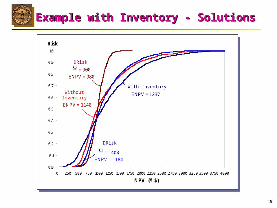
Example with Inventory - SolutionsExample with Inventory - SolutionsExample with Inventory - SolutionsExample with Inventory - Solutions

0.0

0.1

0.2

0.3

0.4

0.5

0.6

0.7

0.8

0.9

1.0

0 250 500 750 1000 1250 1500 1750 2000 2250 2500 2750 3000 3250 3500 3750 4000

NPV (M$)

Risk

PP solut ion

E[NPV ] = 1140 M$PPI solut ion

E[NPV ] = 1237 M$

0.0

0.1

0.2

0.3

0.4

0.5

0.6

0.7

0.8

0.9

1.0

0 250 500 750 1000 1250 1500 1750 2000 2250 2500 2750 3000 3250 3500 3750 4000

NPV (M$)

Risk

= 900

ENPV = 980

= 1400

ENPV = 1184

PPI

ENPV = 1140

PPI

ENPV = 1237

With InventoryWithout

Inventory

DRisk

DRisk

46

Downside Expected ProfitDownside Expected ProfitDownside Expected ProfitDownside Expected Profit

Definition: Definition: Definition: Definition:

0

125

250

375

500

625

750

875

1000

1125

1250

0.0 0.1 0.2 0.3 0.4 0.5 0.6 0.7 0.8 0.9 1.0

Risk

CEP (M$)

PP solut ion

E[NPV ] = 1140 M$

= 900

E[NPV ] = 908 M$

0.0

0.1

0.2

0.3

0.4

0.5

0.6

0.7

0.8

0.9

1.0

250 500 750 1000 1250 1500 1750 2000 2250 2500 2750 3000 3250

NPV (M$)

Risk

= 900 = 1100

PP

Up to 50% of risk (confidence?) the lower ENPV solution has higher profit Up to 50% of risk (confidence?) the lower ENPV solution has higher profit expectations. expectations. Up to 50% of risk (confidence?) the lower ENPV solution has higher profit Up to 50% of risk (confidence?) the lower ENPV solution has higher profit expectations. expectations.

),(),(),(),( ò

¥ xDRiskxRiskdxfpxDENPV xxx

47

Value at RiskValue at RiskValue at RiskValue at Risk

Definition: Definition: Definition: Definition:

VaR=zVaR=zpp for symmetric distributions (Portfolio optimization) for symmetric distributions (Portfolio optimization)VaR=zVaR=zpp for symmetric distributions (Portfolio optimization) for symmetric distributions (Portfolio optimization)

VaR is given by the difference between the mean value of the profit and the profit value corresponding to the p-quantile.

),()]([),( 1 xRiskxProfitEpxVaR

0.00

0.02

0.04

0.06

0.08

0.10

0.12

0.14

Profit x

Area = Risk (x ,)

x fixed

Profit PDF

)]([ xProfitE

),( pxVaR

48

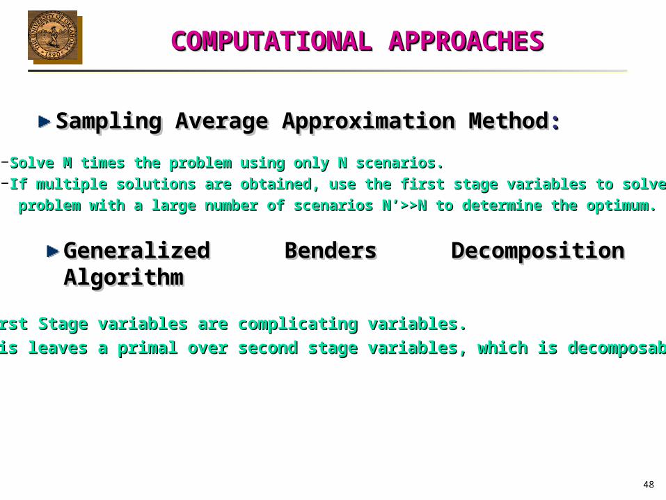
COMPUTATIONAL APPROACHESCOMPUTATIONAL APPROACHESCOMPUTATIONAL APPROACHESCOMPUTATIONAL APPROACHES

Sampling Average Approximation MethodSampling Average Approximation Method::Sampling Average Approximation MethodSampling Average Approximation Method::

−Solve M times the problem using only N scenarios. Solve M times the problem using only N scenarios. −If multiple solutions are obtained, use the first stage variables to solve the If multiple solutions are obtained, use the first stage variables to solve the

problem with a large number of scenarios N’>>N to determine the optimum. problem with a large number of scenarios N’>>N to determine the optimum.

− First Stage variables are complicating variables. First Stage variables are complicating variables. − This leaves a primal over second stage variables, which is decomposable. This leaves a primal over second stage variables, which is decomposable.

Generalized Benders Decomposition Algorithm Generalized Benders Decomposition Algorithm

Generalized Benders Decomposition Algorithm Generalized Benders Decomposition Algorithm

492005 2030

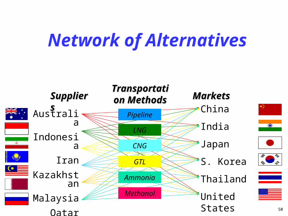
ExampleExample

Generate a model to: Evaluate a large network of natural gas

supplier-to-market transportation alternatives

Identify the most profitable alternative(s)

Manage financial risk

50

Australia

Indonesia

Iran

Kazakhstan

Malaysia

Qatar

Russia

Network of Alternatives

SuppliersSuppliersChina

India

Japan

S. Korea

Thailand

United States

MarketsMarketsTransportation Transportation

MethodsMethods

LNG

CNG

Ammonia

Methanol

Pipeline

GTL

51

Network of Alternatives

52

ResultsResults

Risk Management (Downside Risk):Risk Management (Downside Risk):

0.0

0.1

0.2

0.3

0.4

0.5

0.6

0.7

0.8

0.9

1.0

0 1 2 3 4 5 6 7 8 9 10

1s 4.666

DR-200s4.640

200s 4.678

Malaysia

GTL

ThailandChina

0.0

0.1

0.2

0.3

0.4

0.5

0.6

0.7

0.8

0.9

1.0

0 1 2 3 4 5 6 7 8 9 10

Indo-GTLShips: 5 & 3ENPV:4.633DR@ 4: 0.190DR@ 3.5: 0.086

Mala-GTLShips: 4 & 2ENPV:4.570DR@ 4: 0.157DR@ 3.5: 0.058

53

Value at Risk (VaR):Value at Risk (VaR):

VaR is the expected loss for a certain confidence level usually set at 5% VaR =ENPV – NPV @ p-quantile

Opportunity Value (OV) or Upper Potential (UP):

OV = NPV @ (1-p)-quantile – ENPV

54

ResultsResults

Value at Risk (VaR) and Opportunity Value (OV):Value at Risk (VaR) and Opportunity Value (OV):

Reduction in VaR: 18.1% Reduction in OV: 18.9%

0.0

0.1

0.2

0.3

0.4

0.5

0.6

0.7

0.8

0.9

1.0

0 1 2 3 4 5 6 7 8 9 10



VaR @ 5%: 1.49VaR @ 5%: 1.82

OV @ 95%: 1.75OV @ 95%: 1.42

55

ResultsResults

Risk /Upside Potential Loss RatioRisk /Upside Potential Loss Ratio

0.0

0.1

0.2

0.3

0.4

0.5

0.6

0.7

0.8

0.9

1.0

0 1 2 3 4 5 6 7 8 9 10



VaR @ 5%: 1.49VaR @ 5%: 1.82

OV @ 95%: 1.75OV @ 95%: 1.42

O-Area: 0.116

R-Area: 0.053

Risk /Upside Potential Loss Ratio: 2.2

56

Risk /Upside Potential Loss RatioRisk /Upside Potential Loss Ratio

Risk /Upside Potential Loss Ratio ò

ò¥

¥

¥

¥

dNPV

dNPV

R_Area

O_Area

otherwise

if

0

0

otherwise

if

0

0

)()( NPVRiskNPVRisk DRNGCNGC

where:

0.0

0.1

0.2

0.3

0.4

0.5

0.6

0.7

0.8

0.9

1.0

0 1 2 3 4 5 6 7 8 9 10NPV

Risk

O_Area

R_Area

Risk(x1,NPV)

Risk(x2,NPV)

ENPV1ENPV2

57

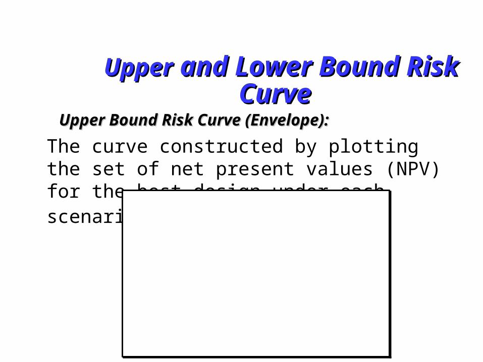
UpperUpper and Lower Bound Risk and Lower Bound Risk CurveCurve

The curve constructed by plotting the set of net present values (NPV) for the best design under each scenario.

Upper Bound Risk Curve (Envelope):Upper Bound Risk Curve (Envelope):

0

0.2

0.4

0.6

0.8

1

0.00 2.00 4.00 6.00 8.00 10.00

Risk

a) Possible

b) Possible

E) Envelope

0

0.2

0.4

0.6

0.8

1

0.0 2.0 4.0 6.0 8.0 10.0

Risk

d) Impossible

c) Impossible

E) Envelope

58

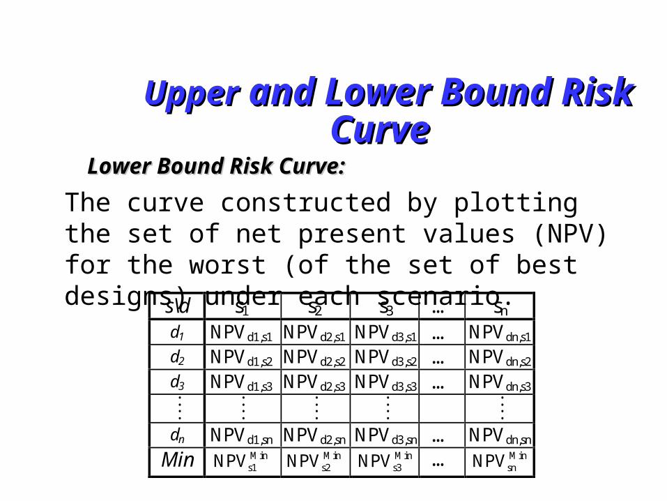
UpperUpper and Lower Bound Risk and Lower Bound Risk CurveCurve

The curve constructed by plotting the set of net present values (NPV) for the worst (of the set of best designs) under each scenario.

Lower Bound Risk Curve:Lower Bound Risk Curve:

s\d s1 s2 s3 … sn d1 NPVd1,s1 NPVd2,s1 NPVd3,s1 … NPVdn,s1

d2 NPVd1,s2 NPVd2,s2 NPVd3,s2 … NPVdn,s2

d3 NPVd1,s3 NPVd2,s3 NPVd3,s3 … NPVdn,s3 : :

: :

: :

: :

: :

dn NPVd1,sn NPVd2,sn NPVd3,sn … NPVdn,sn

Min Mins1NPV Min

s2NPV Mins3NPV … Min

snNPV

59

ResultsResults UpperUpper and Lower Bound Risk and Lower Bound Risk

CurveCurve

0.0

0.2

0.4

0.6

0.8

1.0

0.0 1.0 2.0 3.0 4.0 5.0 6.0 7.0 8.0 9.0

Indo-GTLShips: 6 & 3ENPV:4.63

Mala-GTLShips: 4 & 3ENPV:4.540

Upper EnvelopeENPV:4.921

Lower EnvelopeENPV:3.654

60

ConclusionsConclusionsConclusionsConclusions

A probabilistic definition of Financial Risk has been introduced in the A probabilistic definition of Financial Risk has been introduced in the framework of two-stage stochastic programming. Theoretical properties offramework of two-stage stochastic programming. Theoretical properties ofrelated to this definition were explored.related to this definition were explored.

A probabilistic definition of Financial Risk has been introduced in the A probabilistic definition of Financial Risk has been introduced in the framework of two-stage stochastic programming. Theoretical properties offramework of two-stage stochastic programming. Theoretical properties ofrelated to this definition were explored.related to this definition were explored.

Using downside risk leads to a model that is decomposable in scenarios and thatUsing downside risk leads to a model that is decomposable in scenarios and thatallows the use of efficient solution algorithms. For this reason, it is suggested allows the use of efficient solution algorithms. For this reason, it is suggested that this model be used to manage financial risk.that this model be used to manage financial risk.

Using downside risk leads to a model that is decomposable in scenarios and thatUsing downside risk leads to a model that is decomposable in scenarios and thatallows the use of efficient solution algorithms. For this reason, it is suggested allows the use of efficient solution algorithms. For this reason, it is suggested that this model be used to manage financial risk.that this model be used to manage financial risk.

New formulations capable of managing financial risk have been introduced.New formulations capable of managing financial risk have been introduced.The multi-objective nature of the models allows the decision maker to chooseThe multi-objective nature of the models allows the decision maker to choosesolutions according to his risk policy. The cumulative risk curve is used as asolutions according to his risk policy. The cumulative risk curve is used as atool for this purpose.tool for this purpose.

To overcome the mentioned computational difficulties, the concept of DownsideTo overcome the mentioned computational difficulties, the concept of DownsideRisk was examined, finding that there is a close relationship between thisRisk was examined, finding that there is a close relationship between thismeasure and the probabilistic definition of risk.measure and the probabilistic definition of risk.

To overcome the mentioned computational difficulties, the concept of DownsideTo overcome the mentioned computational difficulties, the concept of DownsideRisk was examined, finding that there is a close relationship between thisRisk was examined, finding that there is a close relationship between thismeasure and the probabilistic definition of risk.measure and the probabilistic definition of risk.

The models using the risk definition explicitly require second-stage binary The models using the risk definition explicitly require second-stage binary variables. This is a major limitation from a computational standpoint.variables. This is a major limitation from a computational standpoint.The models using the risk definition explicitly require second-stage binary The models using the risk definition explicitly require second-stage binary variables. This is a major limitation from a computational standpoint.variables. This is a major limitation from a computational standpoint.

An example illustrated the performance of the models, showing how the riskAn example illustrated the performance of the models, showing how the riskcurves can be changed in relation to the solution with maximum expected profit.curves can be changed in relation to the solution with maximum expected profit.An example illustrated the performance of the models, showing how the riskAn example illustrated the performance of the models, showing how the riskcurves can be changed in relation to the solution with maximum expected profit.curves can be changed in relation to the solution with maximum expected profit.

1 FINANCIAL RISK CHE 5480 Miguel Bagajewicz University of Oklahoma School of Chemical Engineering...

Documents

Transcript of 1 FINANCIAL RISK CHE 5480 Miguel Bagajewicz University of Oklahoma School of Chemical Engineering...