1

Equivalence and Bioequivalence:Frequentist and Bayesian views

on sample size

Mike Campbell

ScHARR

CHEBS FOCUS fortnight 1/04/03

2

Equivalence

• Many trials are not designed to prove differences but equivalences

Examples : generic drug vs established drug

Video vs psychiatrist

NHS Direct vs GP

Costs of two treatments

Alternatively – non-inferiority (one-sided)

3

Efficacy vs cost

• For some trials (e.g. of generics) one would like to show similar efficacy at less cost

• Thus can have an equivalence and a cost difference trial in one study

4

Motivating example

• AHEAD (Health Economics And Depression)

• Trial of trycyclics, SSRIs and lofepramine• Clinical outcome - depression free months• Economic outcome – cost• Powered to show equivalence to within 5%

with 90% power and 5% significance (estimated effect size 0.3 and SD 1.0)

5

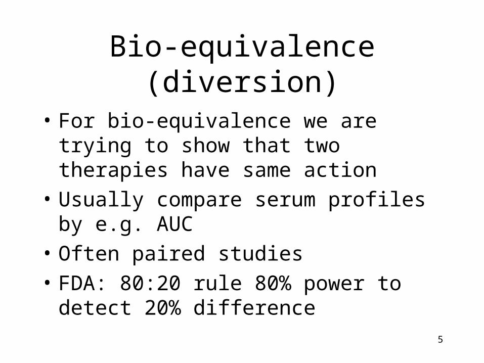
Bio-equivalence (diversion)

• For bio-equivalence we are trying to show that two therapies have same action

• Usually compare serum profiles by e.g. AUC

• Often paired studies

• FDA: 80:20 rule 80% power to detect 20% difference

6

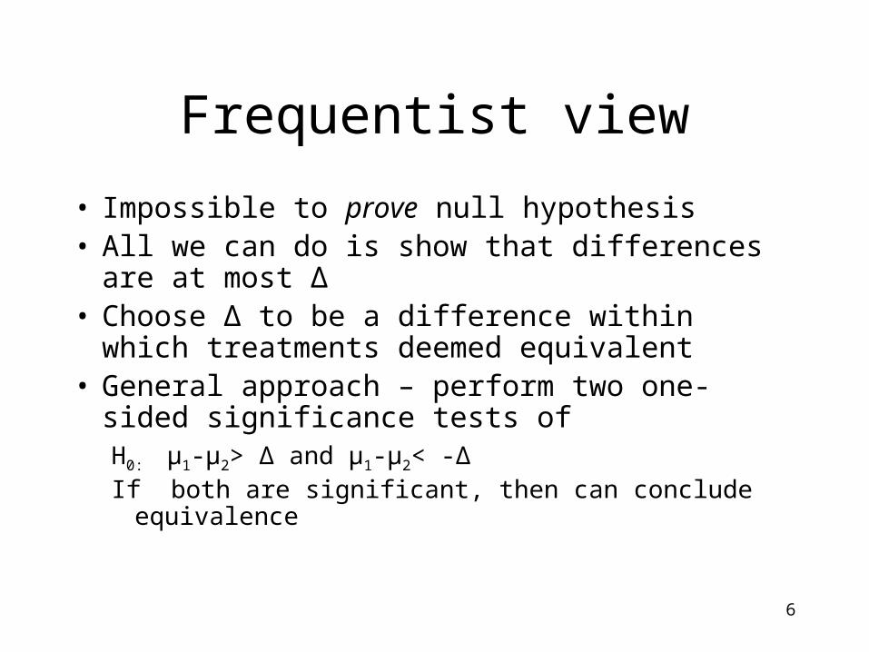
Frequentist view

• Impossible to prove null hypothesis• All we can do is show that differences are at most Δ• Choose Δ to be a difference within which treatments

deemed equivalent• General approach – perform two one-sided

significance tests of H0: μ1-μ2> Δ and μ1-μ2< -ΔIf both are significant, then can conclude equivalence

7

Figure from Jones et al (BMJ 1996) showing relationshipbetween equivalence and confidence intervals

8

CIs

2/2/ , zdzd

Assume sd is known.

Then 100(1-)% CI to compare difference in means is

Treatments deemed equivalent if interval falls in-Δ to +Δ

2/112

11 )( nnwhere

9

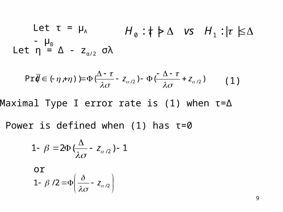
Let τ = μA - μB ||:|:| 10 HvsH

Let η = Δ - zα/2 σλ

)()()),(Pr( 2/2/

zzd

Power is defined when (1) has τ=0

(1)

1)(21 2/

z

2/2/1

z

or

Maximal Type I error rate is (1) when τ=Δ

10

If treatment groups have same size, n, then required sample size is

22/2/2

2

)(2

zzn a

This is similar to testing for a difference

Excepti) Usually Δ is smaller than for a difference trialii) We use β/2 rather than β

(2)

11

Problems with equivalence trials

• Poor trials (e.g. poor compliance and larger measurement errors bias trial towards null)

• Jones et al (1996) suggest using an ITT approach and ‘per-protocol’ and hope they give similar results!

12

Bayesian sample size (O’Hagan and Stevens 2001)

• Analysis objective Outcome is positive if the data obtained are such that there is a posterior probability of at least ω that τ >0

• Design objective We require the sample size (n1,n2) be large enough so there is a probability of at least ψ of obtaining a positive result.

The probability ψ is known as the assurance

13

Bayesian assumptions

• Let prior expectation of (μ1,μ2)T be ma according to analysis prior and md according to the design prior

• Let variances be Va and Vd for analysis and design priors respectively

• Let be ( )T, the observed data• Let S be the sampling variance matrix (note

this depends on n1 and n2)

x 21 , xx

14

Let Wa =Va-1 ,Ws=S-1 and V*=(Wa+Ws)-1 and a=(1,-1)T

)xWm{WVa saa*T

Posterior mean of (μ1, μ2) is Normally distributed with expectation and variance

aVa *T

Under analysis prior

15

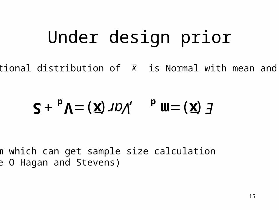
Under design prior

S V x m xd d ) ( , ) (Var E

Unconditional distribution of is Normal with mean and variancex

From which can get sample size calculation (See O Hagan and Stevens)

16

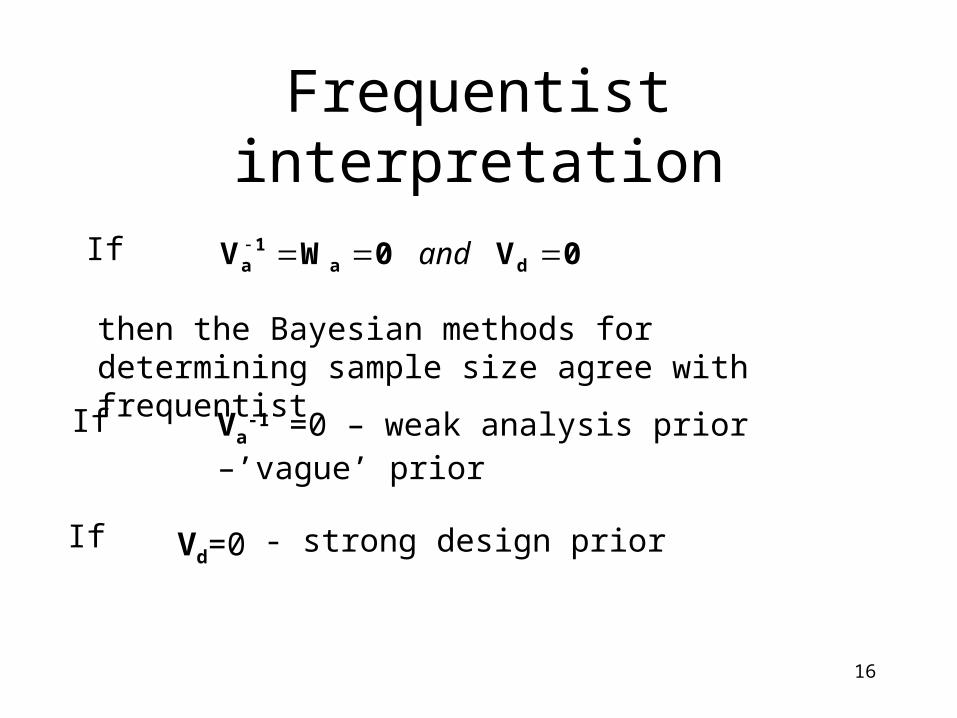
Frequentist interpretation

If 0V0WV da1

a and

then the Bayesian methods for determining sample size agree with frequentist

Va-1 =0 – weak analysis prior –’vague’ prior

If Vd=0

If

- strong design prior

17

Bayesian equivalence (after O’Hagan and Stevens(2001)

• Analysis objective: Outcome of study is positive if the upper limit of the (1-ω)% prediction interval for τ is < Δ (one sided) or upper and lower limits of prediction interval for τ are within ± Δ (two sided).

• Design objective: Sample size is such that there is a probability of at least ψ of obtaining a positive result.

18

aVa)xWm{WVa *Tsaa

*T 1|| z

A modification of O’Hagan and Stevens suggests that for equivalence trials, a positive outcome occurs when

aVa)xWm{WVa *Tsaa

*T 1z

Two-sided and

One-sided

Sample size also a modification of O’Hagan and Stevens

19

Parameters for non-inferiority

ma - the analysis prior mean could be 0

md - the design prior mean could be 0

20

What if md and Vd>0 ?A weak design prior

Then we have some information about the possible differences, so ‘proving’ the null hypothesis is difficult

E.g. if we were 50% sure that δ>0, before the trialthen cannot be 80% sure that δ=0 after the trial

21

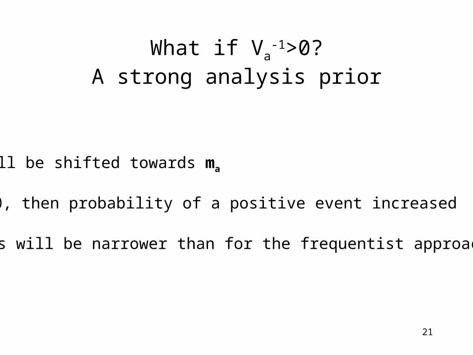
What if Va-1>0?

A strong analysis prior

CIs will be shifted towards ma

If ma=0, then probability of a positive event increased 95% CIs will be narrower than for the frequentist approach

22

Conclusions

• Bayesian approach more natural for equivalence (Can prove H0)

• More work on getting pragmatic suggestions for Va and Vd needed