1

ECON 240C

Lecture 8

2

Part I. Economic Forecast Project

• Santa Barbara County Seminar– April 17, 2003

• URL: http://www.ucsb-efp.com

3

Part II. Forecasting Trends

4

Lab Two: LNSP500

5

Note: Autocorrelated Residual

6

Autorrelation Confirmed from the Correlogram of the Residual

7

Visual Representation of the Forecast

8

Numerical Representation of the Forecast

9

Note: The Fitted Trend Line Forecasts Above the Observations

10

One Period Ahead Forecast

• Note the standard error of the regression is 0.2237

• Note: the standard error of the forecast is 0.2248

• Diebold refers to the forecast error– without parameter uncertainty, which will just

be the standard error of the regression– or with parameter uncertainty, which accounts

for the fact that the estimated intercept and slope are uncertain as well

11

Parameter Uncertainty

• Trend model: y(t) = a + b*t + e(t)

• Fitted model: tbay *ˆˆˆ tbaty *ˆˆ)(ˆ

12

Parameter Uncertainty

• Estimated error )(ˆ)()(ˆ tytyte

13

Forecast Formula

• )1()1(*ˆˆ)1(ˆ tetbaty

14

Forecast

• Et

)1(*

)1()1(*ˆˆ)1(ˆ

tba

tetbaty

15

Forecast

• Forecast = a + b*(t+1) + 0

Ety )1(ˆ )1(ˆ ty

)1()1(*)ˆ()ˆ()1(ˆ)1(ˆ tetbbaatyEty t

16

Variance in the Forecast Error

)1Re()1(*ˆ)1(*ˆˆ*2]ˆ[

)1(ˆ)1(ˆ[2

tVAtbVARtbaCOVaaVAR

tyEtyVAR t

17

18

Variance of the Forecast Error

)1Re()1(*ˆ)1(*ˆˆ*2]ˆ[

)1(ˆ)1(ˆ[2

tVAtbVARtbaCOVaaVAR

tyEtyVAR t

0.000501 +2*(-0.00000189)*398 + 9.52x10-9*(398)2 +(0.223686)2

0.000501 - 0.00150 + 0.001508 + 0.0500354 0.505444SEF = (0.505444)1/2 = 0.22482

19

Numerical Representation of the Forecast

20

21

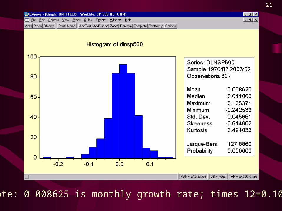
Note: 0 008625 is monthly growth rate; times 12=0.1035

22

Is the Mean Fractional Rate of Growth Different from Zero?

• Econ 240A, Ch.12.2

• where the null hypothesis is that = 0.

• (0.008625-0)/(0.045661/3971/2)

• 0.008625/0.002292 = 3.76 t-statistic, so 0.008625 is significantly different from zero

)//()( nsx

23

Model for lnsp500(t)

• Lnsp500(t) = a +b*t +resid(t), where resid(t) is close to a random walk, so the model is:

• lnsp500(t) a +b*t + RW(t), and taking expontial

• sp500(t) = ea + b*t + RW(t) = ea + b*t eRW(t)

24

Part III. Autoregressive Representation of a Moving Average Process

• MAONE(t) = WN(t) + a*WN(t-1)

• MAONE(t) = WN(t) +a*Z*WN(t)

• MAONE(t) = [1 +a*Z] WN(t)

• MAONE(t)/[1 - (-aZ)] = WN(t)

• [1 + (-aZ) + (-aZ)2 + …]MAONE(t) = WN(t)

• MAONE(t) -a*MAONE(t-1) + a2 MAONE(t-2) + .. =WN(t)

25

• MAONE(t) = a*MAONE(t-1) - a2*MAONE(t-2) + …. +WN(t)

26

Lab 4: Alternating Pattern in PACF of MATHREE

27

Part IV. Significance of Autocorrelations

•

x, x (u) ~ N(0, 1/T) , where T is # of observations x, x (u) ~ N(0, 1/T) , where T is # of observations

28

Correlogram of the Residual from the Trend Model for LNSP500(t)

29

Box-Pierce Statistic

xx,)(ˆ

)/1/()0)(ˆ(

,

,

uT

Tu

xx

xx

Is normalized, 1.e. is N(0,1)

The square of N(0,1) variables is distributed Chi-square

)(ˆ ,2 uT xx

30

Box-Pierce StatisticThe sum of the squares of independent N(0, 1) variables is Chi-square, and if the autocorrelations are close to zero they will be independent, so under the null hypothesis that the autocorrelations are zero, we have a Chi-square statistic:

)(ˆ1

,2 uT

K

u

xx

that has K-p-q degrees of freedom where K is the number of lags in the sum, and p+q are the number of parameters estimated.

31

Application to Lab Four: the Fractional Change in the Federal Funds Rate

• Dlnffr = lnffr-lnffr(-1)

• Does taking the logarithm and then differencing help model this rate??

32

33

34

Correlogram of dlnffr(t)

35

How would you model dlnff(t) ?

• Notation (p,d,q) for ARIMA models where d stands for the number of times first differenced, p is the order of the autoregressive part, and q is the order of the moving average part.

36

Estimated MAThree Model for dlnffr

37

Correlogram of Residual from (0,0,3) Model for dlnffr

38

Calculating the Box-Pierce Stat

Lag ACF ACF square SUM Sum*5841 0.013 0.000169 0.000169 0.0986962 -0.015 0.000225 0.000394 0.2300963 -0.026 0.000676 0.00107 0.624884 -0.004 0.000016 0.001086 0.6342245 -0.029 0.000841 0.001927 1.125368

39

EVIEWS Uses the Ljung-Box Statistic

40

Q-Stat at Lag 5

• (T+2)/(T-5) * Box-Pierce = Ljung-Box

• (586/581)*1.25368 = 1.135 compared to 1.132(EVIEWS)

41

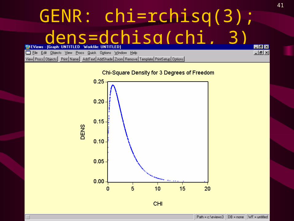
GENR: chi=rchisq(3); dens=dchisq(chi, 3)

42

Correlogram of Residual from (0,0,3) Model for dlnffr

43