1 EBMUD-152

1 __________________________________________________________________________________________

TESTIMONY OF DR. BENJAMIN S. BRAY, Ph.D, P.E.

1

2

3

4

5

6

7

8

9

10

11

12

13

14

15

16

17

18

19

20

21

22

23

24

25

26

27

28

CRAIG S. SPENCER, SBN 78277 General Counsel FRED S. ETHERIDGE, SBN 125095 Assistant General Counsel JONATHAN D. SALMON, SBN 265681 Attorney Office of General Counsel East Bay Municipal Utility District 375 Eleventh Street (MS 904) P.O. Box 24055 Oakland, California 94623-1055 Telephone: (510) 287-0174 Facsimile: (510) 287-0162 [email protected] [email protected] ROBERT E. DONLAN, SBN 186185 SHAWNDA M. GRADY, SBN 289060 Ellison, Schneider & Harris L.L.P. 2600 Capitol Avenue, Suite 400 Sacramento, California 95816 Telephone: (916) 447-2166 Facsimile: (916) 447-3512 [email protected] [email protected] Attorneys for EAST BAY MUNICIPAL UTILITY DISTRICT

BEFORE THE

CALIFORNIA STATE WATER RESOURCES CONTROL BOARD

HEARING IN THE MATTER OF CALIFORNIA DEPARTMENT OF WATER RESOURCES AND UNITED STATES BUREAU OF RECLAMATION REQUEST FOR A CHANGE IN POINT OF DIVERSION FOR CALIFORNIA WATER FIX

TESTIMONY OF DR. BENJAMIN S. BRAY, Ph.D., P.E.

1 EBMUD-152

2 __________________________________________________________________________________________


1

2

3

4

5

6

7

8

9

10

11

12

13

14

15

16

17

18

19

20

21

22

23

24

25

26

27

28

I, Benjamin S. Bray, do hereby declare:

I. INTRODUCTION AND OVERVIEW OF TESTIMONY

I am a Senior Civil Engineer employed by the East Bay Municipal Utility District

(“EBMUD”). I hold a Bachelor of Science in Environmental Resource Engineering from

Humboldt State University (2000) and a Masters of Science (2002) and Doctor of Philosophy in

Civil Engineering with an emphasis in water resources and minors in operations research and

linear statistical models (2006) from the University of California at Los Angeles. I am a

registered Civil Engineer in the State of California (C78883), and I have over nine years of

experience with EBMUD. A true and correct copy of my statement of qualifications is submitted

as EBMUD-127.

In this testimony, I present my analysis and findings regarding potential impacts of the

California WaterFix Project (“WaterFix Project”) on the operation of the Freeport Regional

Water Project (“Freeport Project”). The Freeport Project is owned and operated by the Freeport

Regional Water Authority, a joint powers authority of EBMUD and the Sacramento County

Water Agency (“SCWA”). Based on my review and analysis of the modeling results provided

for this proceeding by the California Department of Water Resources (“DWR”) and the United

States Bureau of Reclamation (“USBR”) (collectively, “Petitioners”), I conclude that, under

certain circumstances, the WaterFix Project is likely to increase the frequency and duration of

reverse flow events in the Sacramento River that exceed threshold criteria that require the

Freeport Project intake facility to temporarily stop diverting water.

The Joint Change Petition (“Change Petition”) filed by Petitioners on August 26, 2015

contains no analysis of the WaterFix Project’s potential impacts on the Freeport Project. Nor did

Petitioners present any such analysis in their written testimony and exhibits filed in support of

the Change Petition. Therefore, to determine whether the WaterFix Project may impede the

Freeport Project’s operation, I performed a technical analysis of the modeling results generated

by Petitioners for this hearing from the CalSim-II and Delta Simulation Model II (“DSM2”)

//

//

2 EBMUD-152

3 __________________________________________________________________________________________


1

2

3

4

5

6

7

8

9

10

11

12

13

14

15

16

17

18

19

20

21

22

23

24

25

26

27

28

models.1 Specifically, I analyzed Petitioners’ CalSim-II modeling results for output of monthly

average flows near the Freeport Project intake for Water Years 1922 through 2003 under each of

the five modeling alternatives Petitioners presented. The five alternatives are the No Action

Alternative and four project alternatives: H3, H4, Boundary 1, and Boundary 2.2 I also analyzed

Petitioners’ DSM2 15-minute velocity output for Water Years 1976 through 1991 to assess the

potential project impact on the frequency of reverse flow events that meet or exceed specified

shutdown criteria for the Freeport Project intake.3

Based on my analysis of the CalSim-II modeling results developed by Petitioners for this

Change Petition, I conclude that the implementation of the WaterFix Project will likely cause

further Sacramento River flow reductions during seasonally dry conditions. These incremental

flow reductions, as compared to the No Action Alternative, result in more frequent reverse flow

events that meet or exceed Freeport Project intake shutdown criteria. Increased Freeport Project

shutdowns will cause operational disturbances and may result in a loss of water supply to

EBMUD and SCWA in critical months during droughts when existing supplies are already

deficient to meet existing needs. DSM2 modeling also indicates that the proposed WaterFix

Project has the potential to cause Freeport Project shutdowns that would not otherwise have

occurred. DSM2 analysis identified 29 months during dry years within Water Years 1976

through 1991 when at least one of the four project alternatives will increase the frequency of

1 Petitioners’ May 16, 2016 letter to the hearing officers notified the parties of the public availability of “updated modeling relating to the proposed project and modeling on an adaptive operational range.” EBMUD subsequently requested that modeling from Petitioners, and I have relied on the modeling Petitioners provided in response to EBMUD’s request to prepare this testimony. 2 For a description of the CalSim-II and DSM2 models as well as additional information on the five alternatives modeled for the Change Petition, refer to testimonies of Jennifer Pierre (Exhibit DWR-51), Parviz Nader-Tehrani (Exhibit DWR-66), and Armin Munévar (Exhibit DWR-71), and the exhibits referenced in each. 3 Although Petitioners also provided DSM2 modeling results for Water Year 1975, I excluded the Water Year 1975 output data from my analysis to allow a “warm up” period. This approach is consistent with Petitioners’ decision not to use Water Year 1975 data, as explained by Petitioners’ DSM2 expert, Dr. Parviz Nader-Tehrani, during cross-examination.

3 EBMUD-152

4 __________________________________________________________________________________________


1

2

3

4

5

6

7

8

9

10

11

12

13

14

15

16

17

18

19

20

21

22

23

24

25

26

27

28

reverse flow events that meet or exceed the Freeport Project intake shutdown criteria, as

compared to the No Action Alternative.

Taken together, the CalSim-II and DSM2 models demonstrate the potential for

Petitioners to shift existing operations upon implementation of the WaterFix Project to alter the

timing of their north-to-south exports within a given year. This change may periodically reduce

freshwater flows at Freeport, causing more reverse flow events that meet or exceed the Freeport

Project intake shutdown criteria.

Section I of this testimony presents this overview of my conclusions. Section II describes

how tidal influences affect the Freeport Project intake by causing reverse flows and explains how

the Freeport Project must shut down during certain reverse flow events. In Section III, I outline

the technical approach I used to analyze the WaterFix Project’s impact on reverse flows at

Freeport, utilizing results from two models, CalSim-II and DSM2. Section IV presents the

findings from my analysis of the modeling performed by Petitioners in connection with the

Change Petition. Section V discusses uncertainties and model limitations of this analysis.

Finally, Section VI presents several conceptual permit terms that would remedy the injury to

EBMUD and SCWA.

II. BACKGROUND

A. Tidal Cycle Influence on Reverse Flows at Freeport.

The Freeport Project intake is located on the Sacramento River near the town of Freeport.

The Sacramento River is a major tributary to the Sacramento-San Joaquin Delta (“Delta”). The

Delta is subject to natural tidal cycles because it is connected to the San Francisco Bay and,

ultimately, the Pacific Ocean. Tidal cycles that drive the rise and fall of large water bodies are a

function of the combined gravitational forces exerted by the Moon, the Sun, and the rotation of

the Earth. The Delta is a “mixed tide” system, meaning that two uneven tidal cycles typically

occur each day with characteristic higher high water, lower high water, higher low water, and

lower low water. This tidal cycle is illustrated in Figure 1.

The extent to which tidal cycles affect the Sacramento River at Freeport depends in part

on the volume of freshwater flows traveling downstream at Freeport. When Sacramento River

4 EBMUD-152

5 __________________________________________________________________________________________


1

2

3

4

5

6

7

8

9

10

11

12

13

14

15

16

17

18

19

20

21

22

23

24

25

26

27

28

freshwater flows are relatively high, tidal influence is more pronounced in downstream reaches,

and tidal influence on discharge measurements at Freeport are small or virtually non-existent.

However, when Sacramento River freshwater flows are relatively low, tidal influence will extend

further up the Sacramento River and up into other Delta tributaries. The tidal influence can even

reverse the flow of the river at Freeport for a period of time when Sacramento River freshwater

flows are relatively low. Figure 1 shows an example of tidal influence resulting in reverse flows

during low tide over a period of three days in April 2015.

B. The Freeport Project Intake Must Shut Down Whenever Reverse Flow

Events Exceed Pre-Determined Threshold Criteria.

Reverse flows can require temporary Freeport Project shutdowns. The Freeport Project

intake is located near a major wastewater discharge point. The Sacramento Regional County

Sanitation District (“Regional San”) discharges treated wastewater into the Sacramento River

through a wastewater outflow diffuser 1.3 miles downstream from the Freeport Project intake.

The discharged wastewater remains downstream of the Freeport Project intake during normal

flow conditions, but it can become a concern during reverse flow conditions.4

When reverse flows occur on the Sacramento River near Freeport, discharged wastewater

from Regional San flows upstream towards the Freeport Project intake. To prevent wastewater

effluent from entering the Freeport Project intake, the Freeport Project must stop diverting water

immediately when Regional San’s wastewater effluent has traveled an average distance of 0.9

miles upstream from its discharge point. This distance of upstream travel is referred to as the

“advective transport distance.” The Freeport Project intake may not resume operation until the

Sacramento River’s flow returns to a normal downstream flow and the wastewater effluent zone

has retreated downstream to a location not more than 0.7 miles upstream from Regional San’s

discharge point. These criteria are contained in a coordinated operations agreement between the

Freeport Regional Water Authority and Regional San, and they are enforceable conditions of the

4 The proposed WaterFix Project’s diversion point nearest the Freeport Project intake is about four miles downstream of the Regional San wastewater discharge point, between the towns of Courtland and Clarksburg, as depicted on Figure 2.

5 EBMUD-152

6 __________________________________________________________________________________________


1

2

3

4

5

6

7

8

9

10

11

12

13

14

15

16

17

18

19

20

21

22

23

24

25

26

27

28

domestic water supply permit issued to EBMUD by the State Water Resources Control Board

(“SWRCB”) Division of Drinking Water.5 Figure 3 contains a graphical representation of the

criteria for shut down and resumption of Freeport Project intake operations during reverse flow

events.

To meet those criteria, the Freeport Project operators must identify tidal influence on the

Sacramento River by monitoring velocities at the Freeport gage around the clock. The Freeport

gage is about 1.3 miles downstream of the Freeport Project intake near the Freeport Bridge. The

gage has operated since at least 1948 and is a semi-continuous monitoring station of river stage,

river discharge, battery voltage, water velocity, water temperature, electrical conductivity, and

water turbidity.

C. Reverse Flow Events that Exceed the Freeport Project’s Mandatory

Shutdown Criteria Have Historically Occurred in Low-Flow Conditions.

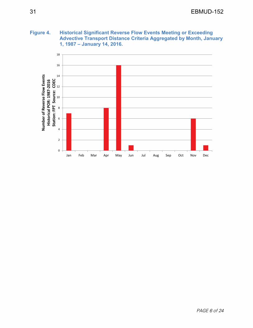
To understand the conditions under which SRFEs may occur, I analyzed publicly-

available data from the Freeport gage.6 As used in this testimony, a “significant reverse flow

event” (“SRFE”) is a reverse flow event that would cause wastewater effluent from Regional San

to travel an average of 0.9 miles or more upstream from its discharge point, which is the

threshold at which the Freeport Project must stop diverting water.

I applied the Freeport Project shutdown criteria to Freeport gage velocity data between

0100 hours on January 1, 1987 through 2400 hours on January 14, 2016. The gage data indicates

that SRFEs corresponded to months with significantly low flows on the Sacramento River, which

typically occurred in critically dry years. The monthly distribution is shown on Figure 4. Figure

5 illustrates the relationship between monthly average flows and the frequency of SRFE

occurrences in the corresponding month. While the sample size is not large, this historical

5 For a detailed discussion of these restrictions, see Exhibit EBMUD-151 (Testimony of Eileen M. White, P.E.) at page 10. 6 I downloaded the historic Freeport gage data (USGS 11447650) from the California Data Exchange Center (“CDEC”), http://cdec.water.ca.gov/queryCSV.html.

6 EBMUD-152

7 __________________________________________________________________________________________


1

2

3

4

5

6

7

8

9

10

11

12

13

14

15

16

17

18

19

20

21

22

23

24

25

26

27

28

analysis shows an increasing incidence of SRFEs as monthly average flow decreases below

8,000 cubic feet per second (“cfs”).

III. ANALYSIS METHODS

My analysis of the potential impacts of the WaterFix Project on the operation of the

Freeport Project and associated facilities focused on Petitioners’ CalSim-II and DSM2 modeling

and the modeling I performed utilizing Petitioners’ models. Petitioners’ CalSim-II modeling

included a longer 82-year period of hydrology (Water Years 1922 through 2003), as compared to

the shorter 16-year DSM2 simulation performed for this proceeding (Water Years 1976 through

1991). The longer period simulated with CalSim-II allows assessment of a wider range of

hydrology and associated operations. A key advantage of DSM2, as compared with CalSim-II,

is its 15-minute velocity output. The modeled velocity at a 15-minute time step is necessary and

sufficient to directly identify short-term, tidally-influenced SRFEs. I describe my CalSim-II and

DSM2 analysis in the remaining portion of this Section III.

A. Petitioners’ CalSim-II Results Were Screened to Identify Months in Which

WaterFix Project Operations Increase the Risk of Significant Reverse Flow

Events at Freeport.

Petitioners used CalSim-II, a water resources planning model, to evaluate the WaterFix

Project and the associated operations of the State Water Project (“SWP”) and the Central Valley

Project (“CVP”). CalSim-II is a monthly model that quantifies river flows, reservoir storage

levels, diversions, return flows, as well as Delta inflows and outflows under various SWP/CVP

operating scenarios.

To determine if the WaterFix Project has the potential to change river flow in a manner

that may increase the frequency and severity of SRFEs, I compared CalSim-II model results for

the Sacramento River immediately downstream of Freeport for the No Action Alternative and

each of the four project alternatives. Specifically, I developed and applied a set of Monthly Flow

Criteria, which is comprised of three logic statements that I applied as a filter to compare

CalSim-II results for the various project alternatives with the No Action Alternative:

//

7 EBMUD-152

8 __________________________________________________________________________________________


1

2

3

4

5

6

7

8

9

10

11

12

13

14

15

16

17

18

19

20

21

22

23

24

25

26

27

28

For each project alternative (H3, H4, Boundary 1, and Boundary 2):

1. the monthly average flow below the Freeport Project intake for the project

alternative is less than the No Action Alternative, and

2. the monthly average flow for the project alternative is less than the threshold

value of 8,000 cfs, and

3. the relative change in monthly average flow between the project alternative and

the No Action Alternative is greater than a tolerance of 20 cfs.

The first logic statement above is intended to flag months in which modeled Freeport

flows in one of several project alternatives are less than modeled flows in the No Action

Alternative.

The second logic statement applies an 8,000 cfs low-flow threshold adopted from my

analysis of historical flows recorded by the Freeport gage station. I described that historical data

analysis in Section II. That analysis indicates that SRFEs historically occur most frequently

when flows drop below 8,000 cfs. On that basis, I applied a criterion of monthly average flow

less than or equal to 8,000 cfs as a reasonable threshold indicator variable for assessing the

potential for the WaterFix Project to increase the risk of SRFEs.

The third logic statement is simply a tolerance to avoid small changes in monthly average

flow that are not expected to impact reverse flow events. Sensitivity on the magnitude of this

tolerance is also included in my analysis of results below to indicate how it could affect the risk

assessment outcome.

By applying the three Monthly Flow Criteria to screen Petitioners’ CalSim-II monthly

flow output data, I identified specific months in which Petitioners’ WaterFix modeling results

indicate that at least one WaterFix Project alternative would reduce flows at Freeport by more

than a nominal amount during the type of low-flow conditions historically associated with

SRFEs.

To be clear, the months flagged by the Monthly Flow Criteria do not necessarily equate

to SRFEs. SRFEs cannot be directly identified from the CalSim-II model output. The strength of

a given reverse flow event is a function of several factors, including Sacramento River flow, the

8 EBMUD-152

9 __________________________________________________________________________________________


1

2

3

4

5

6

7

8

9

10

11

12

13

14

15

16

17

18

19

20

21

22

23

24

25

26

27

28

specific characteristics of the natural tidal cycle, and operation of key downstream facilities such

as the Delta Cross Channel. Detailed modeling of these parameters is not available through

CalSim-II. One readily available CalSim-II model output, however, is the monthly average flow

immediately downstream of the Freeport Project intake. I used that flow information to identify

the relative change in risk of increased reverse flow events due to the WaterFix Project

significantly lowering Sacramento River flows relative to the No Action Alternative. This

approach is an appropriate comparative analysis that utilizes the CalSim-II monthly output to

assess the project effect on the risk of incurring SRFEs that would impact Freeport Project intake

operations.

B. Petitioners’ DSM2 Results Were Analyzed With and Without Bias

Correction to Identify Discrete Significant Reverse Flow Events Resulting

from WaterFix Project Operations that Impact the Freeport Project.

1. Overview of DSM2 Methodology

Petitioners used DSM2 to simulate the No Action Alternative and the four WaterFix

Project alternatives. DSM2 simulates flow, velocity, stage, and electric conductivity. Petitioners

included certain analysis of stage and electric conductivity in their exhibits and written

testimony. Petitioners did not provide an analysis of velocity data but did make available the

DSM2 15-minute velocity output for Water Years 1976 through 1991. That velocity data can be

used to directly assess the effect of the WaterFix Project on Freeport Project intake operations. I

compared simulated DSM2 velocity data from Petitioners’ historical simulation with actual

velocity data from the Freeport gage station data. That comparison revealed that Petitioners’

DSM2 results systematically under-predicted peak velocity magnitudes at high and low tide.

To correct that under-prediction bias, I calculated an appropriate velocity offset to apply

to Petitioners’ DSM2 velocity output to match minimum reverse flow velocities. I calculated the

optimal offset by minimizing the sum-of-square error between model simulation and historical

Freeport gage data over 15 months of historical low-flow periods in which reverse flow events

//

//

9 EBMUD-152

10 __________________________________________________________________________________________


1

2

3

4

5

6

7

8

9

10

11

12

13

14

15

16

17

18

19

20

21

22

23

24

25

26

27

28

occurred.7 I applied the optimal offset to the simulated output to align as closely as possible with

the actual velocities recorded by the Freeport gage. Applying that offset produced a set of bias-

corrected velocity output for assessing reverse-flow impacts derived from the DSM2 output

provided by Petitioners. This offset is key because the negative 15-minute velocity output is the

basis for calculating the shutdown criteria triggered by the Freeport gage station. If the

simulated peak minimum reverse flow velocity is underestimated, then the modeling results will

systematically underestimate SRFEs.

I analyzed both the non-bias-corrected output and the bias-corrected output to identify

discrete SRFEs in each data set. I describe my methodology in greater detail in the remainder of

this portion of my testimony.

2. Method of Analysis of Non Bias-Corrected Velocity Output

I first analyzed Petitioners’ DSM2 velocity output data without bias correction. For each

reverse flow event (i.e. when velocity is negative), I computed the advective transport distance

by multiplying the velocity (feet per second) by the time step (seconds). Whenever the

accumulated advective transport distance for the reverse flow event met or exceeded 0.9 miles

(4,752 feet), I identified that event as a SRFE that would cause a shutdown of the Freeport

Project intake. I screened from the results all “non-significant” reverse flow events: those in

which the accumulated advective transport distance did not meet the 0.9 mile threshold, because

such reverse flow events would not trigger a shutdown of the Freeport Project intake. I then

compared SRFEs identified for each of the four project alternatives to the No Action Alternative

to determine whether the WaterFix Project would negatively impact EBMUD and SCWA’s

ability to take diversions through the Freeport Project. I describe the results of that analysis in

Section IV of my testimony.

//

//

7 These were the months of October and November 1990, February 1991, May 1991, May through August 1992, October and November 1992, April through June 1994, December 2008, and November 2009.

10 EBMUD-152

11 __________________________________________________________________________________________


1

2

3

4

5

6

7

8

9

10

11

12

13

14

15

16

17

18

19

20

21

22

23

24

25

26

27

28

3. Bias Correction of DSM2 Velocity Output

Because the DSM2 model consistently underrepresents peak reverse flows at Freeport, I

developed and applied a bias correction offset to the raw DSM2 velocity output data. This offset

adjusted the simulated velocities to more closely match expected minimum velocities during

reverse flow events based on actual Freeport gage station records.

The DSM2 model does not accurately simulate velocity at Freeport at peak high tide or at

peak low tide. In both cases, DSM2 tends to understate the peak amplitude. For example,

during reverse flow events, DSM2 simulates a reverse flow that is weaker than would

realistically occur under the simulated conditions. I identified this bias by plotting Freeport

velocity output data generated by Petitioners’ DSM2 calibration run against actual velocity data

recorded in the same location by the Freeport gage during the simulated period. Two examples

from May 1991 and November 1992 are depicted in Figure 6. These graphs show the DSM2

model’s continuous under-prediction of river velocities at peak tides. Of direct relevance to

reverse flow analysis, the graphs included in Figure 6 specifically show that this under-prediction

occurs during reverse flow conditions. In other words, actual measured velocities are

consistently more strongly negative than DSM2 has simulated. This means that SRFEs are

actually more frequent, and more severe, than estimated from uncorrected DSM2 output. For

that reason, I believe that Petitioners’ uncorrected DSM2 output data should not be relied upon to

determine the impact of the WaterFix Project on the Freeport Project intake.

Instead, a bias correction offset should be applied to match the low-amplitude peak

reverse flow velocities with the velocities actually observed at Freeport. I developed a bias

offset of -0.230 feet per second by minimizing the sum-of-square error between simulated and

recorded peak minimum velocities for the Freeport gage over a 15-month period of historical

records in which flows were low enough to contain reverse flow events at the gaging station. I

then applied the offset to the 16-year set of velocity output data at the Freeport Project intake.

Figure 7 illustrates how applying the offset caused the simulated velocity data to more closely

match observed actual reverse flow conditions at Freeport during the reverse flow period when

velocity is negative. In my opinion, that bias-corrected data provides a significantly more

11 EBMUD-152

12 __________________________________________________________________________________________


1

2

3

4

5

6

7

8

9

10

11

12

13

14

15

16

17

18

19

20

21

22

23

24

25

26

27

28

accurate representation of the Sacramento River’s velocity at Freeport under the simulated

conditions, and therefore it should be relied upon to analyze the WaterFix Project’s impact on

shutdown events at the Freeport Project intake.

The uncorrected DSM2 velocity data is not reliable for SRFE analysis. DSM2 is

calibrated with the “big picture” of the Delta and all its complexity in mind; it is calibrated to

simulate a broad range of criteria under a wide array of conditions. With limitations inherent to

any modeling application, model calibration involves tradeoffs in criteria, especially for large

and complex systems. By calibrating with the “big picture” in mind, criteria-specific or localized

biases are inevitably introduced. When using the model for a specific purpose – in this case, to

identify SRFEs – it is both appropriate and necessary to calculate and apply bias correction to

maximize the simulation’s accuracy in representing reverse flow events for the Freeport gage

station. Bias-corrected data derived for reverse-flow analysis purposes should not be used for

other purposes (for example, it should not be used to identify peak positive flows), but it is the

best available dataset to comparatively analyze reverse flows.

After applying the bias correction to velocity data for the full 16-year simulated period to

both the No Action Alternatives and the four project alternatives, I identified additional SRFEs

not discerned from the uncorrected velocity data. Section IV provides the results of that

analysis.

IV. IMPACT ANALYSIS RESULTS AND DISCUSSION

Through my analysis of the WaterFix Project CalSim-II and DSM2 modeling prepared by

Petitioners for this hearing, I conclude that the WaterFix Project will likely cause an increase in

the frequency and duration of SRFEs that will result in an increase in the frequency and duration

of shutdowns of the Freeport Project intake. These impacts are most likely to occur in critically

dry years, during the periods in which EBMUD relies on Freeport Project water. This

conclusion is based on my analysis of Petitioners’ CalSim-II modeling, applying the Monthly

Flow Criteria as described above, together with the results of my analysis of Petitioners’ DSM2

modeling. My conclusion is consistent with the results of prior independent modeling analysis

efforts described below in Section IV.D.

12 EBMUD-152

13 __________________________________________________________________________________________


1

2

3

4

5

6

7

8

9

10

11

12

13

14

15

16

17

18

19

20

21

22

23

24

25

26

27

28

A. CalSim-II Simulations of WaterFix Project Operations Indicate An

Increased Risk of Significant Reverse Flow Events During Low-Flow

Periods.

I applied the Monthly Flow Criteria over the 82-year period of record as described in

Section III.A. As indicated in Table 1, I determined from that analysis that 34 months meet all

Monthly Flow Criteria for the H3 project simulation, 22 months meet all Monthly Flow Criteria

for the H4 project simulation; 22 months meet all Monthly Flow Criteria for the Boundary 1

simulation; and 20 months meet all Monthly Flow Criteria for the Boundary 2 simulation. These

are months in which the WaterFix Project increases the risk of Freeport Project intake

shutdowns. As shown in Table 1, such months tend to occur during drought periods. Table 1

provides the total number of months that meet the Monthly Flow Criteria during each of the three

major drought periods over the modeled 82-year period: 1929-1934, 1976-1977, and 1987-

1992.8 Depending on which project alternative is analyzed, the WaterFix Project increases the

risk of SRFEs relative to the No Action Alternative in 7% to 16% of months during the three

identified drought periods.

I also analyzed the sensitivity on the 20 cfs tolerance parameter incorporated into the

Monthly Flow Criteria by varying this parameter from a minimum of 0 cfs to a maximum of 150

cfs. Sensitivity results showed that any tolerance parameter between 0 cfs and 150 cfs results in

at least a 5% increase in the number of months that meet the Monthly Flow Criteria during the

three drought periods identified in Table 1 under all project alternatives relative to the No Action

Alternative. This sensitivity analysis demonstrates that the result obtained from application of

the Monthly Flow Criteria is relatively insensitive to the choice of the monthly flow tolerance

parameter. Among the project alternatives, the H3 simulation was most sensitive to the choice of

tolerance parameter, decreasing from 15% to 8.7% as the tolerance parameter increases from 0

8 For purposes of my analysis, the identified major drought periods commence with the first month of the first dry water year and continue through the month in which the Sacramento River monthly average flow begins to increase with the onset of winter storms at the beginning of the subsequent wet year. The terminal months for these three droughts were October 1934, November 1977, and November 1992.

13 EBMUD-152

14 __________________________________________________________________________________________


1

2

3

4

5

6

7

8

9

10

11

12

13

14

15

16

17

18

19

20

21

22

23

24

25

26

27

28

cfs to 150 cfs. In contrast, the Boundary 1 alternative was least sensitive to the choice of

tolerance parameter, decreasing from 8.1% to 6.9% over the same range.

B. DSM2 Simulations Show that WaterFix Project Operations Will Impact the

Timing and Frequency of Significant Reverse Flow Events.

I analyzed the DSM2 modeling studies to assess SRFEs directly for the 16-year period

simulated by Petitioners (Water Years 1976 through 1991). I did this analysis twice: without

bias correction and with bias correction. In both cases, I found the WaterFix Project would alter

the pattern of SRFE occurrences, as compared with the No Action Alternative.

1. Analysis of Uncorrected DSM2 Velocity Output Data

Table 2 identifies the total number of modeled SRFEs during the 16-year DSM2

simulation period for the No Action Alternative and each modeled WaterFix Project alternative.

Table 2 is based on an analysis of uncorrected raw output data exactly as provided by Petitioners.

As shown in that table, the large majority of SRFEs during that period occurred during the

droughts in 1976-1977 and 1987-1992. Because dry, low-flow conditions continued into Water

Year 1992 – the final year of the latter drought – it is likely that additional SRFEs occurred that

year. However, my analysis does not include SRFEs during that water year because Petitioners

did not model this sixth year of the drought with DSM2.

Without bias correction applied, the DSM2 analysis reveals a modest overall decrease in

SRFEs in each of the four project alternatives in relation to the No Action Alternative. During

the 1976-1977 drought, all project alternatives remain within ±4 SRFEs relative to the No Action

Alternative. The H4 alternative shows an increase of two SRFEs during that drought. During

the simulated portion of the 1987-1992 drought (i.e., excluding Water Year 1992), all project

alternatives show a decrease relative to the No Action Alternative.

2. Analysis of Bias-Corrected DSM2 Velocity Output Data

Following my analysis of uncorrected velocity data, I then applied the -0.230 feet per

second (ft/sec) offset to correct the model’s reverse flow under-prediction bias, and analyzed the

corrected data to identify SRFEs under the No Action Alternative and each project alternative.

Table 3 presents the results of the analysis of the corrected data. A comparison of Table 3 with

14 EBMUD-152

15 __________________________________________________________________________________________


1

2

3

4

5

6

7

8

9

10

11

12

13

14

15

16

17

18

19

20

21

22

23

24

25

26

27

28

Table 2 reveals the significance of the DSM2 bias. Table 3 shows a much greater incidence of

SRFEs under all five modeled alternatives than Table 2. Although the No Action Alternative

and the project alternatives all reflect this increase, the corrected modeling results show that

SRFEs have the potential for a greater impact on the Freeport Project than the uncorrected

modeling results would suggest. It also shows that the WaterFix Project operation will require a

greater number of shutdowns of the Freeport Project intake than previously understood, and,

therefore, a commensurately greater degree of impact to EBMUD and SCWA.

Table 3 shows a moderate overall decrease in SRFEs under the project alternatives during

drought periods relative to the No Action Alternative. Note that Table 3, unlike Table 2, shows

increased SRFEs during the 1976-1977 drought in three of four project alternatives simulated.

Comparing overall SRFE totals alone does not adequately convey the totality of the

WaterFix Project’s impact on the Freeport Project. Because impacts may depend upon not only

how many SRFEs occur, but also upon when they occur, I analyzed patterns in the distribution of

SRFEs throughout the year, comparing the No Action Alternative with the project alternatives.

Aggregating SRFEs by month, as I present in Figure 8, reveals how WaterFix Project operations

could lead to a disproportionate share of SRFE impacts in some months. The DSM2 analysis

shows a tendency for SRFEs to increase relative to the No Action Alternative in a few different

ways. There are small changes among the project scenarios in January through April. There

tends to be a small decrease in May and June with Boundary 2 showing the smallest change

relative to the No Action Alternative. There is not much change in July, and SRFEs would

decrease significantly under all project alternatives in August due to increases in Sacramento

River flows. September through December show a higher potential for increased SRFEs over

various project alternatives. In September, the H3, H4, and Boundary 1 project alternatives all

increase SRFEs significantly relative to the No Action Alternative, while September SRFEs

would decrease under Boundary 2. A comparison of project alternatives with the No Action

Alternative also shows increases for H3 in October and Boundary 2 in December. Figure 8

shows that operation of the WaterFix Project will likely impact the timing of SRFEs – most

prominently in fall and winter months before storm events occur.

15 EBMUD-152

16 __________________________________________________________________________________________


1

2

3

4

5

6

7

8

9

10

11

12

13

14

15

16

17

18

19

20

21

22

23

24

25

26

27

28

C. A Comparative Analysis of the CalSim-II and DSM2 Modeling Shows How

Shifted Export Patterns Will Change Flows and Thereby Increase Significant

Reverse Flow Events, Especially During Drought Periods.

After I analyzed Petitioners’ CalSim-II and DSM2 modeling separately, I analyzed the

results from both models together to understand how changes in flows simulated in CalSim-II

translate to changes in SRFE impacts on the Freeport Project intake simulated in DSM2.

1. Comparison of Flow Data and SRFEs

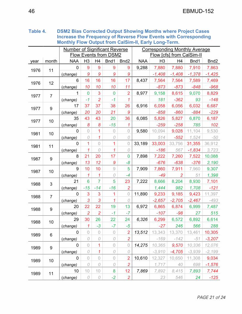
My comparative analysis revealed 29 separate months during the 1976-1991 period

simulated by Petitioners in which one or more of the four project alternatives would increase

SRFEs relative to the No Action Alternative, listed in Table 4. These 29 months are the months

during the DSM2 modeling period when the WaterFix Project could cause additional shutdowns

of the Freeport Project intake. The impacts tend to become more frequent as drought periods

progress. For example, 1977 has a higher proportion of SRFEs than 1976. Similarly, 1990 and

1991 had more SRFEs than 1987 and 1988. These impacts are clearly concentrated in droughts

when the Sacramento River freshwater flows are lowest. Table 4 also shows that at least one

project alternative increases SRFEs in every month between December 1990 and August 1991,

except May 1991.

Table 4 directly compares the DSM2 and CalSim-II analysis for each modeled

alternative. The -0.230 ft/sec offset was applied to the DSM2 output data for the No Action

Alternative and all project alternatives. Table 4 includes all months in which DSM2 analysis,

after application of the offset, indicates that at least one project alternative would increase the

number of SRFEs relative to the No Action Alternative. The left portion of the table indicates

the number of SRFEs under the DSM2 modeling for each modeled alternative. The portion of

the table on the right provides corresponding monthly average flow information from CalSim-II,

including flows in the No Action Alternative, each project alternative, and the difference relative

to the No Action Alternative.

The data provided in Table 4 supports the incorporation into the Monthly Flow Criteria of

8,000 cfs monthly average flow below Freeport as a reasonable threshold indicator of SRFE

16 EBMUD-152

17 __________________________________________________________________________________________


1

2

3

4

5

6

7

8

9

10

11

12

13

14

15

16

17

18

19

20

21

22

23

24

25

26

27

28

potential for time periods when DSM2 data is not available. During the months included in

Table 4 – all months when SRFEs would occur – flows at Freeport ranged from a high of 31,355

cfs in November 1981 under Boundary 1 (a flow that corresponds to one modeled SRFE) to a

low of 5,826 cfs in October 1977 under the H3 alternative (a flow that corresponds to 43

SRFEs). Table 4 also shows the lack of a perfect correlation between flows and the number of

SRFEs. For example, under the Boundary 1 simulation, 18 SRFEs occurred in October 1990,

corresponding to a flow of 6,870 cfs, but 28 SRFEs occurred in September 1990 despite slightly

lower flows of 6,842 cfs. While flows are an important factor in determining SRFEs’ number

and severity, tidal and operational characteristics also play a key role.

2. Connection between WaterFix Project SRFE Impacts and Shifts in the

Timing of Exports

Petitioners assert that the WaterFix Project’s purpose is to enhance operational flexibility

for the SWP and CVP through the use of three new points of diversion in the north Delta. The

CalSim-II and DSM2 results, when considered together, show how WaterFix Project operators

could use that new flexibility to shift the timing of north-to-south Delta export patterns. Such

shifts will, at times, result in lower Sacramento River flows, with an accompanying increase in

SRFEs.

I present two months as examples to illustrate this impact: September 1977 and June

1991. I chose these months because they represent two examples where the Delta is in “excess”

and “balanced” conditions, respectively.9 First, I compared the DSM2 modeling under the No

Action Alternative to the H3 project alternative for September 1977. As shown in Table 4 and

Figure 9, DSM2 results for that month indicate that SRFEs increase from 17 under the No Action

Alternative to 37 under H3. CalSim-II indicates that, under H3, the timing of total water exports

“shifts” to earlier in 1977 than under the No Action Alternative. Figure 10 shows this shift in

9 Excess conditions are periods when releases from upstream reservoirs plus unregulated flow exceed Sacramento Valley inbasin uses, plus exports. Balanced conditions are periods when releases from upstream reservoirs plus unregulated flow approximately equal the water supply needed to meet Sacramento Valley inbasin uses, plus exports.

17 EBMUD-152

18 __________________________________________________________________________________________


1

2

3

4

5

6

7

8

9

10

11

12

13

14

15

16

17

18

19

20

21

22

23

24

25

26

27

28

total export timing for those two alternatives. Figure 10 shows that exports increase under the

H3 alternative in April through August and November and December but are reduced in

September and October. The reduction in exports in September and October under the H3

alternative corresponds to decreased Sacramento River flows at Freeport from 6,916 cfs to 6,058

cfs during the same period, as shown on Figure 11.

I also compared the No Action Alternative and Boundary 1 alternative for June 1991.

Again, I found that shifting export patterns resulted in periods with lower flows, which were

associated with an increase in SRFEs. Figure 12 shows the total exports for these two

alternatives and indicates a shift in the timing and quantity of exports under the project

alternative relative to the No Action Alternative. In this case, the Boundary 1 project alternative

shows significantly increased exports in March through May, relative to the No Action

Alternative, along with smaller increases in September through December, coupled with

corresponding decreases in June, July, and August. This corresponds to a decrease in

Sacramento River flows in June, July, and August as shown in Figure 13. The reduced flows

associated with shifting export patterns in June 1991 result in increased SRFEs. Figure 14 shows

the DSM2 velocity output for June 1991 for the No Action Alternative and the Boundary 1

project alternative. Figure 14 shows that operating WaterFix to the Boundary 1 alternative

caused SRFEs to increase from 4 to 12 during June 1991, compared to the No Action

Alternative. Stated another way, 8 new SRFEs occurred in June 1991 that would not occur in the

absence of the WaterFix Project.

These examples from 1977 and 1991 show how the operational flexibility that Petitioners

seek through the WaterFix Project will allow them to shift the timing of exports, which will

cause lower Sacramento River flows at certain times, resulting in more SRFEs at those times

than would have occurred without the WaterFix Project. More broadly, the examples show the

importance of looking beyond raw SRFE totals aggregated over many years to understand how

WaterFix Project will impact the Freeport Project.

//

//

18 EBMUD-152

19 __________________________________________________________________________________________


1

2

3

4

5

6

7

8

9

10

11

12

13

14

15

16

17

18

19

20

21

22

23

24

25

26

27

28

D. My Results are Consistent with Previous Modeling Efforts by DWR and

Independent Modelers that Concluded the North Delta Diversion Will

Impact Significant Reverse Flow Events at Freeport.

The modeling that Petitioners released in May 2016 for this water rights hearing is not

the first time that a project very similar to WaterFix has been modeled. In fact, DWR simulated

the operation of three new intakes of the same capacity, in the same location, with the same or

similar set of assumed bypass flow criteria and other operational limitations used in the WaterFix

Project modeling in 2013 when it performed CalSim-II and DSM2 modeling of the Bay-Delta

Conservation Plan (“BDCP”). The key difference between the BDCP and the WaterFix Project

is that the former project included a suite of environmental measures including tidal marsh

restoration that are not included in the WaterFix Project.

In 2014, EBMUD analyzed DWR’s DSM2 modeling of the BDCP to determine whether

the BDCP would increase SRFEs.10 That analysis showed that 25,000 acres of tidal marsh

restoration would reduce reverse flows at Freeport, even in conjunction with the new north Delta

intakes. However, that analysis also showed that building new intake tunnels without tidal marsh

restoration – as Petitioners now propose to do through the WaterFix Project – would increase

SRFEs at Freeport. The results of EBMUD’s analysis of DWR’s modeling are presented in

Table 5.11 Those results show the BDCP, including tidal marsh restoration, would significantly

reduce the number of SRFEs at Freeport – from 70 to 14, or from 178 to 21, depending on which

planning horizon and associated climate change and sea level rise assumptions were simulated.

A related modeling effort was made by MBK Engineers and Daniel B. Steiner. MBK

and Steiner removed climate change and sea-level rise assumptions from the BDCP CalSim-II

modeling and modeled the new Delta tunnels with and without tidal marsh restoration. EBMUD

then conducted DSM2 modeling of MBK and Steiner’s CalSim-II model results, and analyzed

those DSM2 results to identify how SRFEs are affected by the respective effects of tidal marsh

10 See Exhibit EBMUD-176 (July 28, 2014 comment letter on the BDCP Draft EIS/EIR. 11 This table is taken from Exhibit EBMUD-176, page 176.

19 EBMUD-152

20 __________________________________________________________________________________________


1

2

3

4

5

6

7

8

9

10

11

12

13

14

15

16

17

18

19

20

21

22

23

24

25

26

27

28

restoration and the new Delta tunnels. Table 6 shows the results of EBMUD’s DSM2 modeling

and analysis.12 I draw two conclusions from Table 6. First, the north Delta diversion and the

tidal marsh proposed in the BDCP, when constructed together, would result in a net reduction in

SRFEs at Freeport. Second, in the absence of tidal marsh restoration, operation of new north

Delta intakes would incrementally increase SRFEs from 55 to 64 over a modeled 16-year period.

In other words, the BDCP without restoration would cause SRFEs to increase, which is generally

consistent with the results of my analysis of the WaterFix Project.

V. MODEL LIMITATIONS AND UNCERTANTIES

My analysis demonstrates that the WaterFix Project will likely cause an increase in the

frequency and duration of SRFEs, especially in critical drought months. Although my analysis

relies on Petitioners’ CalSim-II and DSM2 results, I conclude the WaterFix Project may cause

greater SRFE impacts than Petitioners’ modeling predicts – even after correcting for DSM2’s

systematic under-prediction bias of reverse flows. This section of my testimony explains the

basis for my opinion.

A. Petitioners’ Chosen Modeling Methods Do Not Sufficiently Capture

Relatively Rare Events Such as Significant Reverse Flow Events.

CalSim-II is a planning model that operates in broad terms of spatial discretization or

coarse terms in temporal discretization. Such planning models tend to perform poorly in

capturing relatively atypical or rare events. SRFEs are by definition rare events, and thus, not

identified well from CalSim-II modeling. However, CalSim-II is also foundational, meaning that

much of the other modeling for the WaterFix Project is tiered from or built upon the CalSim-II

results, as is the case for the DSM2 model. DSM2 provides model output of velocity on a 15-

minute time step, which allows SRFEs to be directly analyzed where daily averaged results or

monthly results would be insufficient. To perform this analysis, however, CalSim-II and

temporal downscaling techniques are required to map monthly conditions to the temporal scale

required for the DSM2 model simulation. Accordingly, the analysis of 15-minute velocity

12 This table is taken from Exhibit EBMUD-176, page 177.

20 EBMUD-152

21 __________________________________________________________________________________________


1

2

3

4

5

6

7

8

9

10

11

12

13

14

15

16

17

18

19

20

21

22

23

24

25

26

27

28

output from DSM2, even in a comparative sense, is necessarily limited because the CalSim-II

monthly results are a significant factor in assigning boundary conditions to the DSM2 model.

B. DSM2 Insufficiently Modeled Reverse Flows Because of Inherent Model

Limitations, and the Model Was Inadequately Modified to Properly

Represent the Proposed Project Changes.

DSM2 is not the best available tool to analyze reverse flow impacts. DSM2 is a one-

dimensional hydrodynamic model of flow, velocity, stage, and electric conductivity. The single

linear dimension does not accurately represent the complexity of hydrodynamic alterations due

to the three proposed north Delta intakes on the Sacramento River. Two- or three-dimensional

modeling of this region of the Sacramento River would provide a clearer picture of the WaterFix

Project’s impacts, including effects on hydrodynamics and specifically reverse flows and

velocity.

Petitioners also failed to modify DSM2 cross-sections to represent physical changes to

the river channel cross-sections that are proposed as part of the WaterFix Project. For example,

Petitioners did not modify DSM2 to account for the modifications to levees and to represent the

intake structures. Petitioners also failed to modify roughness coefficients to represent the

reduction in roughness expected to result from replacing levees with massive fish screen intakes.

Those changes – the physical modifications and the reduced roughness – would tend to increase

velocity of reverse flow events. This increase is not captured in Petitioners’ modeling.

C. The CalSim-II and DSM2 Models Are Unable to Account for the Broad

Range of Operational Flexibility Afforded by the WaterFix Project.

Petitioners modeled four project alternatives, which they claim represent the full range of

reasonably foreseeable operational possibilities. Those four alternatives – H3, H4, Boundary 1,

and Boundary 2 – each contain operational assumptions. Essentially, those assumptions define

the outer limits of the modeled domain and constrain the results of Petitioners’ modeling. That

constraint would not be objectionable if the modeled scenarios truly represented the full range of

plausible operational scenarios. However, each of Petitioners’ modeled alternatives assumes an

unwarranted and artificial degree of constraint on the project operators’ ability to release water

21 EBMUD-152

22 __________________________________________________________________________________________


1

2

3

4

5

6

7

8

9

10

11

12

13

14

15

16

17

18

19

20

21

22

23

24

25

26

27

28

from storage during summer and fall. In fact, Petitioners’ modeling does not reflect the full

extent of operational flexibility afforded by the WaterFix Project, which would enable operators

to move stored water through the Delta while meeting all flow criteria and water quality

objectives to an extent that is currently not possible. For a detailed discussion of this issue, see

the testimony of Walter Bourez of MBK Engineers, which the Sacramento Valley Water Users

have submitted into the record for this water rights hearing. Mr. Bourez’s conclusions have

important implications for SRFEs at Freeport. The WaterFix Project can be operated to “shift”

the timing of exports to a greater degree than is revealed by Petitioners’ modeling. If those shifts

are more pronounced, they would be accompanied by periods of lower flows than previously

understood. In turn, those lower flows would generally be expected to increase the frequency

and duration of SRFEs – as discussed in Section IV.C of my testimony above.

Petitioners’ modeling also does not account for temporary urgency change petitions and

orders. The recent drought showed that Petitioners seek and obtain temporary urgency changes.

Temporary urgency changes are not represented in Petitioners’ modeling, and if allowed in the

future, they could cause lower flows on the Sacramento River than simulated by Petitioners’

CalSim-II modeling. Finally, without an operations plan and only the proposed north Delta

bypass flow criteria, limited information is available to assess intake impacts during real-time

operations when reverse flows will need to be addressed.

D. Petitioners’ Brief 16-Year Simulation Period Excludes Several Significant

Low-Flow Events and Therefore Limits the DSM2 Modeling’s Usefulness in

Understanding How the WaterFix Project Will Impact Reverse Flows.

Petitioners’ DSM2 model results are unnecessarily limited by Petitioners’ choice of a 16-

year simulation period. That 16-year period excludes several significant simulated low-flow

months in which SRFEs would be expected to occur, as inferred from the 82-year CalSim-II

simulation. My analysis demonstrates that most low-flow instances occur in the fall, before the

onset of winter storm events, and typically in months near the end of drought periods. For

example, close inspection of the CalSim-II monthly average flow results at Freeport reveals that

the lowest monthly average flows – close to or below 6,000 cfs – occurred in September and

22 EBMUD-152

23 __________________________________________________________________________________________


1

2

3

4

5

6

7

8

9

10

11

12

13

14

15

16

17

18

19

20

21

22

23

24

25

26

27

28

October 1934 and May 1977, and the lowest monthly average flow at Freeport simulated over all

four project alternatives was the Boundary 2 simulation, which identified a flow of only 5,121

cfs in November 1992. However, among the four months highlighted above from 1934, 1977

and 1992, only one of those months – May 1977 – is included in the DSM2 modeled period, and

this month shows an increase in flows under the project alternatives.

VI. PROPOSED PERMIT TERMS OR CONDITIONS

In this section, I propose a few possible ways to alleviate the WaterFix Project’s potential

to impact the Freeport Project’s intake operations. This section is not intended to be an

exhaustive set of options; rather, it is presented merely to demonstrate that there are alternatives

not addressed by Petitioners that could reduce the WaterFix Project’s impact on EBMUD and

SCWA.

A. Require Adequate Tidal Marsh Restoration to Mitigate the WaterFix

Project’s Impact on Significant Reverse Flow Events at Freeport.

Petitioners’ water rights permits could be conditioned on Petitioners’ construction of tidal

marsh in a quantity and at a location that is demonstrated by modeling to be sufficient to

completely prevent the anticipated increase in SRFEs at the Freeport Project intake. The Bay-

Delta Conservation Plan (“BDCP”) modeling studies show that construction of a sufficient

acreage of tidal marsh will mitigate the potential reverse flow effects on the Sacramento River

near Freeport. Petitioners’ BDCP Early Long Term (“ELT”) simulations analyzed the impact of

25,000 acres of tidal marsh restoration. Restoration on that scale was effective in significantly

reducing reverse flows on the Sacramento River. Table 6 quantifies the dramatic impact of

large-scale tidal marsh restoration. A smaller-scale restoration project may be sufficient to

prevent the WaterFix Project from causing SRFE impacts. However, additional studies would be

needed to optimize the acreage and location of a sufficient tidal marsh restoration project.

//

//

//

//

23 EBMUD-152

24 __________________________________________________________________________________________


1

2

3

4

5

6

7

8

9

10

11

12

13

14

15

16

17

18

19

20

21

22

23

24

25

26

27

28

B. Require New or Enhanced Bypass Flow Criteria to Ensure that Freshwater

Flows are Sufficient to Mitigate the WaterFix Project’s Impact on Significant

Reverse Flow Events at Freeport.

A minimum flow criterion at Freeport could be placed into Petitioners’ water rights

permits that is sufficient to prevent an increase in SRFEs at Freeport. However, a singular flow

prescription would likely be too rigid a requirement, as there should be some consideration for

environmental conditions such as the natural tidal cycle. Alternatively, Petitioners’ proposed

north Delta bypass flow criteria could be modified such to ensure that minimum flows

downstream of the new north Delta intakes remain sufficient to dampen tidal effects further

upstream on the Sacramento River. Additional studies would be needed to develop a Freeport

bypass flow requirement that is sufficiently protective to eliminate any increase in SRFEs while

maintaining the greatest possible degree of flexibility for the WaterFix Project. Specifically,

analysis would be needed to assess which flows are required under different tidal conditions and

for different Delta Cross Channel operations.

C. Require Petitioners to Provide Additional Water to Compensate for Impacts

from Significant Reverse Flows Events at Freeport.

Petitioners’ permits could be conditioned to require Petitioners to provide additional

water to EBMUD or SCWA, as applicable, when SRFEs occur. This “make-up” water would

then be made available later in the contract year. This would incentivize project operators to

adaptively manage the SWP and CVP projects to minimize SRFEs, and when unavoidable,

provide for and coordinate the delivery of make-up water to compensate for lost supplies when

the Freeport Project intake is shut down. Project operators are skilled and experienced in

managing the projects under real-time conditions. Project operators would likely be able to

adaptively manage the system to minimize SRFEs and consider the tradeoff between shifting

diversion patterns against the risk of necessarily providing make-up water supplies if offsets in

diversions are necessary at other times of the year.

//

//

24 EBMUD-152

1 VII. CONCLUSION

2 The WaterFix Project, as currently proposed, would increase the frequency and duration,

3 and impact the timing, of SRFEs at Freeport Project intake, which will require additional

4 shutdowns. However, protective terms and conditions could be included in Petitioners' water

5 rights to mitigate those SRFE-related impacts.

6

7 Executed this 31st day of August, 2016 in Oakland, California.

8

9

10

11

12

13

14

15

16

17

18

19

20

21

22

23

24

25

26

27

28

25


25 EBMUD-152

of 24

FIGURES and TABLES

26 EBMUD-152

of 24

FIGURES 1—14

27 EBMUD-152

of 24

Figure 1. Tidal Characteristics with Freeport Gage Discharge, April 19-21, 2015. Source: http://cdec.water.ca.gov/ Station “FPT”, on an hourly basis.

28 EBMUD-152

http://cdec.water.ca.gov/

of 24

Figure 2. Map Showing Approximate Locations of Freeport Regional Water Project Intake Facility in Relation to Sacramento Regional County Sanitation District and Proposed Intakes for CAWF.

29 EBMUD-152

of 24

Figure 3. Graphical Representation of Reverse Flow Event Criteria for FRWP Intake Shutdown and Startup in Relation to Regional San and FRWA Facilities. Note locations are approximate for illustrative purposes.

30 EBMUD-152

of 24

Figure 4. Historical Significant Reverse Flow Events Meeting or Exceeding Advective Transport Distance Criteria Aggregated by Month, January 1, 1987 – January 14, 2016.

0

2

4

6

8

10

12

14

16

18

Jan Feb Mar Apr May Jun Jul Aug Sep Oct Nov Dec

Num

ber o

f Rev

erse

Flo

w E

vent

sHi

stor

ical

PO

R: 1

987-

2016

Stat

ion:

FPT

Sou

rce:

CDE

C

31 EBMUD-152

of 24

Figure 5. Calculated Monthly Average Flow and Corresponding Number of Reverse Flow Events that Meet Advective Transport Distance Criteria, January 1, 1987 – January 14, 2016.

0

2

4

6

8

10

12

0 2,000 4,000 6,000 8,000 10,000 12,000 14,000

Num

ber o

f Rev

erse

Flo

w E

vent

s, H

isto

rical

PO

R:

1987

-201

6, S

tatio

n: F

PT S

ourc

e: C

DEC

Calculated Monthly Average Sacramento River Flow at Freeport, Station: FPT, Source: CDEC

Increasing risk of reverse flow events

32 EBMUD-152

of 24

Figure 6. Freeport Gage Velocity with DSM2 Historical Simulated Velocity at Freeport Project Intake, (a) May 1991 and (b) November 1992.

(a)

(b)

-0.5

-0.3

-0.1

0.1

0.3

0.5

0.7

0.9

1.1

1.3

1.5

01-May-91 06-May-91 11-May-91 16-May-91 21-May-91 26-May-91 31-May-91

Velo

city

[ft/

se]

Freeport Gage DSM2 Model May 1991

-0.5

-0.3

-0.1

0.1

0.3

0.5

0.7

0.9

1.1

1.3

1.5

01-Nov-92 06-Nov-92 11-Nov-92 16-Nov-92 21-Nov-92 26-Nov-92 01-Dec-92

Velo

city

[ft/

sec]

Freeport Gage DSM2 Model November 1992

33 EBMUD-152

of 24

Figure 7. Freeport Gage Velocity with DSM2 Historical Simulated Velocity at Freeport Project Intake and DSM2 Velocity with -0.230 ft/sec Bias Correction Offset, Feb. 9 – 27, 1991.

-0.5

-0.2

50

0.250.

5

0.751

1.251.

5

1.75 2/

9/91

2/10

/91

2/11

/91

2/12

/91

2/13

/91

2/14

/91

2/15

/91

2/16

/91

2/17

/91

Velocity [ft/sec]

FPT

Gage

DSM

2 O

utpu

tDS

M2

Bias

Cor

rect

ed

34 EBMUD-152

of 24

Figure 8. Significant Reverse Flow Events from Petitioner’s Bias Corrected DSM2 Simulation of WYs 1976-1991 Aggregated by Month.

0

20

40

60

80

100

120

Jan Feb Mar Apr May Jun Jul Aug Sep Oct Nov Dec

Sign

ifica

nt R

ever

se F

low

Eve

nts

NAA

PA-H3

PA-H4

PA-Bnd1

PA-Bnd2

35 EBMUD-152

of 24

Figure 9. DSM2 Simulated Velocity at Freeport Intake, September 1977 for (a) NAA Scenario (N=17) and (b) H3 Project Alternative (N=37). Green arrows indicate significant reverse flow events that meet or exceed Freeport Project intake shutdown criteria.

(a)

(b)

-1.5

-1

-0.5

0

0.5

1

1.5

9/1/77 9/6/77 9/11/77 9/16/77 9/21/77 9/26/77 10/1/77

DSM

2 Si

mul

ated

Vel

ocity

[ft/

sec]

Significant Reverse Flow Events

-1.5

-1

-0.5

0

0.5

1

1.5

9/1/77 9/6/77 9/11/77 9/16/77 9/21/77 9/26/77 10/1/77

DSM

2 Si

mul

ated

Vel

ocity

[ft/

sec]


36 EBMUD-152

of 24

Figure 10. Total Exports for NAA and H3 Project Alternative, October 1976 – December 1977. Total Exports for Project Alternative are North + South diversions and from south Delta only for NAA.

0

1,000

2,000

3,000

4,000

5,000

6,000

7,000

Oct-76 Nov-76 Dec-76 Jan-77 Feb-77Mar-77 Apr-77 May-77 Jun-77 Jul-77 Aug-77 Sep-77 Oct-77 Nov-77 Dec-77

Tota

l Exp

ort [

cfs]

NAA H3

37 EBMUD-152

of 24

Figure 11. Sacramento River Flow Downstream of FRWP Intake for NAA and H3 Project Alternative, October 1977 – December 1977.

5,000

6,000

7,000

8,000

9,000

10,000

11,000

Oct-76 Nov-76 Dec-76 Jan-77 Feb-77Mar-77 Apr-77 May-77 Jun-77 Jul-77 Aug-77 Sep-77 Oct-77 Nov-77

Flow

Dow

nstr

eam

of F

reep

ort I

ntak

e [c

fs]

NAA H3

38 EBMUD-152

of 24

Figure 12. Total Exports for NAA and Boundary 1 Project Alternative, October 1990 – December 1991. Total exports for Boundary 1 are north + south diversions and from south Delta only for NAA.

0

1,000

2,000

3,000

4,000

5,000

6,000

7,000

8,000

Oct-90 Nov-90 Dec-90 Jan-91 Feb-91 Mar-91 Apr-91 May-91 Jun-91 Jul-91 Aug-91 Sep-91 Oct-91 Nov-91 Dec-91

Tota

l Exp

orts

[cfs

]

NAA Bnd1

39 EBMUD-152

of 24

Figure 13. Sacramento River Flow Downstream of FRWP Intake for NAA and Boundary 1 Scenarios, October 1990 – September 1991.

5,000

10,000

15,000

20,000

25,000

30,000

Oct-90 Nov-90 Dec-90 Jan-91 Feb-91 Mar-91 Apr-91 May-91 Jun-91 Jul-91 Aug-91 Sep-91

Flow

Dow

nstr

eam

of F

reep

ort I

ntak

e [c

fs] NAA Bnd1

40 EBMUD-152

of 24

Figure 14. DSM2 Simulated Velocity at Freeport Intake, June 1990 for (a) NAA (N=4) and (b) Boundary 1 Project Alternative (N=12). Green arrows indicate significant reverse flow events which met or exceed Freeport Project intake shutdown criteria.

(a)

(b)

-2

-1.5

-1

-0.5

0

0.5

1

1.5

2

6/1 6/6 6/11 6/16 6/21 6/26 7/1

DSM

2 Si

mul

ated

Vel

ocity

[ft/

sec]


-2

-1.5

-1

-0.5

0

0.5

1

1.5

6/1 6/6 6/11 6/16 6/21 6/26 7/1

DSM

2 Si

mul

ated

Vel

ocity

[ft/

sec]


41 EBMUD-152

of 24

TABLES 1—6

42 EBMUD-152

of 24

Table 1. Project Effect Frequency Analysis on Low Monthly Flows at Freeport Applying the Monthly Flow Criteria (MFC). Data represents the number of months in which evaluation criteria are met.

Project Alternative H3 H4 Boundary 1 Boundary 2

1929-1934 Drought (Oct. 1928 – Oct. 1934, N = 73) 9 7 6 5

1976-1977 Drought (Oct. 1975 – Nov. 1977, N = 26) 4 4 3 4

1987-1992 Drought (Oct. 1986 – Nov. 1992, N = 74) 12 5 5 8

Drought Subtotal (N = 173) 25 16 14 17 WY 1922 – 2003 Totals (N = 984) 34 22 22 20

43 EBMUD-152

of 24

Table 2. Significant Reverse Flow Events for California WaterFix Water Rights Hearing Modeling Studies. Period of analysis is indicated in parenthesis.

No Action Alternative

Project Scenario H3 H4 Boundary 1 Boundary 2

1976–1977 Drought (Oct. 1975 – Oct. 1977) 31 30 33 27 28

1987–1992α Drought (Oct. 1987 – Sep. 1990) 71 51 45 50 56

WYs 1976–1991 Total (Oct. 1975 – Sep. 1991) 113 89 86 82 96

α - Note that WY 1992 is not included in Petitioners DSM2 modeling simulation, therefore, this final year of the drought cannot be included in the analysis.

44 EBMUD-152

of 24

Table 3. Significant Reverse Flow Events for California WaterFix Water Rights Hearing Modeling Studies from Bias Corrected DSM2 Output. Period of analysis is indicated in parenthesis.

No Action Alternative

Project Scenario H3 H4 Boundary 1 Boundary 2

1976–1977 Drought (Oct. 1975 – Oct. 1977) 165 183 183 160 176

1987–1992α Drought (Sep. 1987 – Sep. 1991) 377 374 332 326 328

WYs 1976–1991 Total (Oct. 1975 – Sep. 1991) 596 572 541 500 504

α - Note that WY 1992 is not included in Petitioners DSM2 modeling simulation, therefore, this final year of the drought cannot be included in the analysis.

45 EBMUD-152

of 24

Table 4. DSM2 Bias Corrected Output Showing Months where Project Cases Increase the Frequency of Reverse Flow Events with Corresponding Monthly Flow Output from CalSim-II, Early Long-Term.

Number of Significant Reverse Flow Events from DSM2

Corresponding Monthly Average Flow [cfs] from CalSim-II

year month NAA H3 H4 Bnd1 Bnd2 NAA H3 H4 Bnd1 Bnd2

1976 11 0 9 9 9 9 9,288 7,880 7,880 7,910 7,863 (change) 9 9 9 9 -1,408 -1,408 -1,378 -1,425

1976 12 6 16 16 16 17 8,437 7,564 7,564 7,589 7,469 (change) 10 10 10 11 -873 -873 -848 -968

1977 7 1 0 3 0 2 8,977 9,158 8,615 9,070 8,829 (change) -1 2 -1 1 181 -362 93 -148

1977 9 17 37 37 38 26 6,916 6,058 6,056 6,032 6,687 (change) 20 20 21 9 -858 -860 -884 -229

1977 10 35 43 43 20 36 6,085 5,826 5,827 6,870 6,187 (change) 8 8 -15 1 -259 -258 785 102

1981 10 0 0 1 0 0 9,580 10,094 9,028 11,104 9,530 (change) 0 1 0 0 514 -552 1,524 -50

1981 11 0 1 0 1 0 33,189 33,003 33,756 31,355 36,912 (change) 1 0 1 0 -186 567 -1,834 3,723

1987 9 8 21 20 17 0 7,898 7,222 7,260 7,522 10,088 (change) 13 12 9 -8 -676 -638 -376 2,190

1987 10 9 10 10 9 5 7,909 7,860 7,911 7,960 9,307 (change) 1 1 0 -4 -49 2 51 1,398

1988 3 21 6 7 5 23 7,222 8,666 8,204 8,930 7,101 (change) -15 -14 -16 2 1,444 982 1,708 -121

1988 7 0 3 3 1 0 11,890 9,233 9,185 9,423 11,397 (change) 3 3 1 0 -2,657 -2,705 -2,467 -493

1988 9 20 22 22 19 13 6,972 6,865 6,874 6,999 7,487 (change) 2 2 -1 -7 -107 -98 27 515

1988 10 29 30 26 22 24 6,326 6,299 6,572 6,892 6,614 (change) 1 -3 -7 -5 -27 246 566 288

1989 6 0 0 0 0 2 13,512 13,343 13,370 13,461 10,305 (change) 0 0 0 2 -169 -142 -51 -3,207

1989 9 0 0 1 0 0 14,275 10,365 9,570 10,336 12,076 (change) 0 1 0 0 -3,910 -4,705 -3,939 -2,199

1989 10 0 0 0 0 2 10,610 12,327 10,650 11,308 9,034 (change) 0 0 0 2 1,717 40 698 -1,576

1989 11 10 10 10 8 12 7,869 7,892 8,415 7,893 7,744 (change) 0 0 -2 2 23 546 24 -125

46 EBMUD-152

of 24

Table 4. cont.

Number of Significant Reverse Flow Events from DSM2

Corresponding Monthly Average Flow [cfs] from CalSim-II

year month NAA H3 H4 Bnd1 Bnd2 NAA H3 H4 Bnd1 Bnd2

1989 12 18 18 0 18 19 7,601 7,728 9,049 7,717 7,418 (change) 0 -18 0 1 127 1,448 116 -183

1990 5 25 27 25 26 26 7,148 7,148 7,159 7,194 7,188 (change) 2 0 1 1 0 11 46 40

1990 9 16 23 20 28 11 7,353 7,092 7,364 6,842 7,889 (change) 7 4 12 -5 -261 11 -511 536

1990 10 36 38 31 18 31 6,060 6,012 6,407 6,870 6,382 (change) 2 -5 -18 -5 -48 347 810 322

1990 12 17 18 18 3 27 7,178 7,132 7,190 9,703 6,471 (change) 1 1 -14 10 -46 12 2,525 -707

1991 1 22 2 1 23 21 6,562 10,699 10,922 6,541 6,618 (change) -20 -21 1 -1 4,137 4,360 -21 56

1991 2 1 12 7 1 7 11,551 8,819 9,054 10,684 9,607 (change) 11 6 0 6 -2,732 -2,497 -867 -1,944

1991 3 0 1 1 0 0 26,936 27,099 27,116 27,147 27,040 (change) 1 1 0 0 163 180 211 104

1991 4 2 3 3 2 3 12,276 12,295 12,314 12,323 12,256 (change) 1 1 0 1 19 38 47 -20

1991 6 4 10 10 12 10 9,694 8,292 8,303 8,107 8,217 (change) 6 6 8 6 -1,402 -1,391 -1,587 -1,477

1991 7 0 2 0 2 0 12,770 9,292 9,367 9,126 11,468 (change) 2 0 2 0 -3,478 -3,403 -3,644 -1,302

1991 8 0 14 14 14 0 8,925 7,833 7,856 7,803 9,584 (change) 14 14 14 0 -1,092 -1,069 -1,122 659

For ease of reference, increases in significant reverse flow events and corresponding monthly flows are colored with red font. Decreases in significant reverse flow events and corresponding monthly flows are colored with green font. For cases where there is no change in the number of significant reverse flow events, grey font is used. Also, italicized font is used for each “change” row of the table where the NAA is subtracted from the project alternative.

47 EBMUD-152

of 24

Table 5. Significant Reverse Flow Analysis of BDCP Project Simulations Excerpted from page 171 of EBMUD’s Comment Letter to the BDCP Dated July 28, 2014. Note period simulated with DSM2 is October 1975 through September 1991 i.e. Water Years 1976 through 1991.

48 EBMUD-152

of 24

Table 6. Independent Outside Modeling of NAA and Project Alternative 4A with and without Tidal-Marsh Restoration Excerpted from page 172 of EBMUD’s Comment Letter to the BDCP Dated July 28, 2014. Note period simulated with DSM2 is October 1921 through September 2003 i.e. Water Years 1922 through 2003 where results for the shorter 16-year period simulated by DWR is also provided for reference. With deactivation of assumptions for climate change (CC) and sealevel rise (SLR), the time basis for the modeling scenarios is rendered moot, hence no indication of the ELT or LLT timeframe.

49 EBMUD-152

1 EBMUD-152

Documents

Transcript of 1 EBMUD-152