1

Design of Engineering ExperimentsPart 4 – Introduction to Factorials

• Text reference, Chapter 5• General principles of factorial experiments• The two-factor factorial with fixed effects• The ANOVA for factorials• Extensions to more than two factors• Quantitative and qualitative factors –

response curves and surfaces

2

Basic Principles and Advantages

• A factorial design – all possible combinations of the levels of the factors are investigated in each complete trial or replication

• Most efficient for two or more factor experiments

• Both main effects and interaction effects can be dealt with

• The effects of a factor can be estimated at several levels of the other factors – wider range of validity of conclusions

3

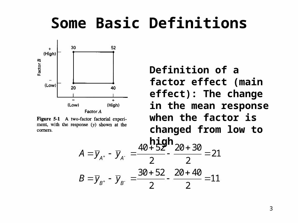
Some Basic Definitions

Definition of a factor effect (main effect): The change in the mean response when the factor is changed from low to high

40 52 20 3021

2 230 52 20 40

112 2

52 20 30 401

2 2

A A

B B

A y y

B y y

AB

4

Some Basic DefinitionsInteraction occurs when differences in response between the levels of one factor is not the same at all levels of the other factors

At the low level of B (B-):

A = 40 – 20 = 20

At the high level of B (B+):

A = 52 – 30 = 22

The magnitude of the interaction effect is the average difference in the two A effects:

12

4030

2

2052

2

2022

2

)()(

BABAAB

5

The Case of Interaction:

50 12 20 401

2 240 12 20 50

92 2

12 20 40 5029

2 2

A A

B B

A y y

B y y

AB

6

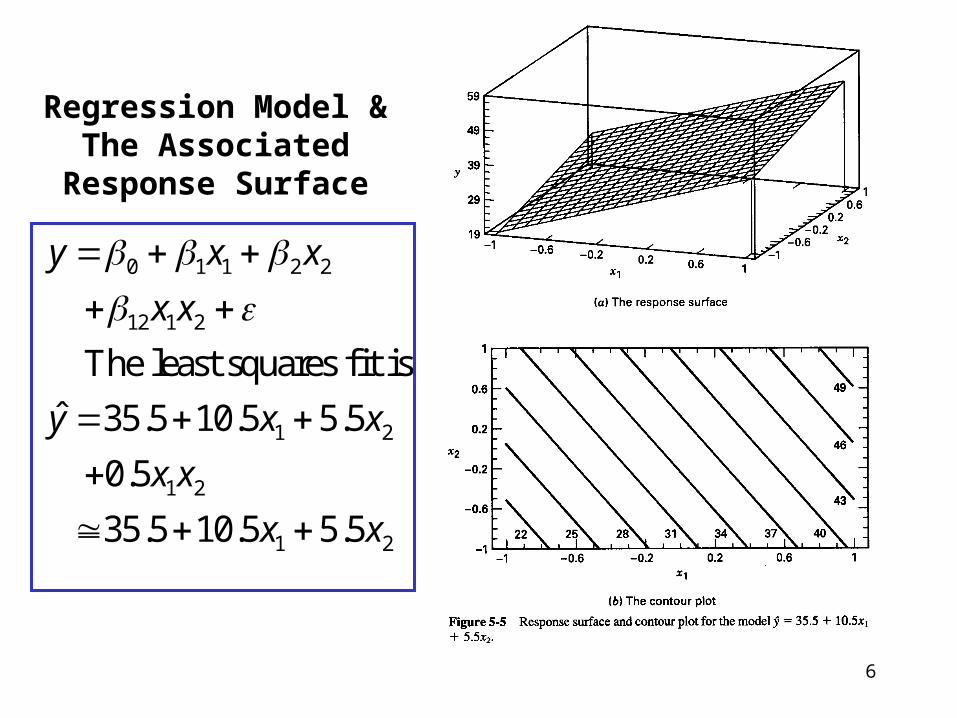
Regression Model & The Associated Response

Surface

0 1 1 2 2

12 1 2

1 2

1 2

1 2

The least squares fit is

ˆ 35.5 10.5 5.5

0.5

35.5 10.5 5.5

y x x

x x

y x x

x x

x x

7

The Effect of Interaction on the Response Surface

Suppose that we add an interaction term to the model:

1 2

1 2

ˆ 35.5 10.5 5.5

8

y x x

x x

Interaction is actually a form of curvature

8

Some Basic Definitions

•The knowledge of the interaction is more useful than knowledge of the main effect•A significant interaction will often mask the significance of main effects.•The main effect of one factor needs to be examined with the levels of other factors fixed when there is a significant interaction•The factorial design is more efficient than one-factor-at-a-time design, and the efficiency increases with the number of factors

9

Example 5-1 The Battery Life ExperimentText reference pg. 175

A = Material type; B = Temperature (A quantitative variable)

1. What effects do material type & temperature have on life?

2. Is there a choice of material that would give long life regardless of temperature (a robust product)?

10

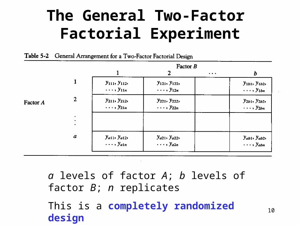
The General Two-Factor Factorial Experiment

a levels of factor A; b levels of factor B; n replicates

This is a completely randomized design

11

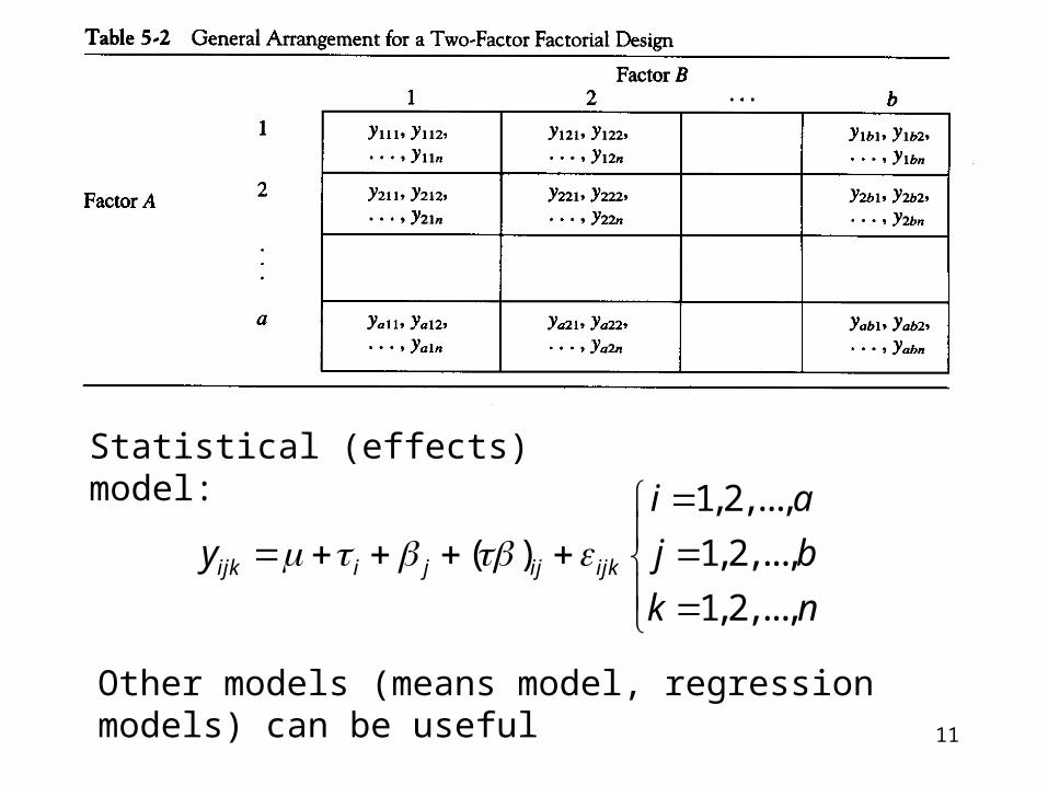
Statistical (effects) model:

1,2,...,

( ) 1,2,...,

1, 2,...,ijk i j ij ijk

i a

y j b

k n

Other models (means model, regression models) can be useful

12

Equality of row treatment effects

Ho: 1 = 2 = = a = 0

H1: at least one i 0

Equality of column treatment effects

Ho: 1 = 2 = = b = 0

H1: at least one j 0

Equality of row and column treatment interactions

Ho: (ij = 0 for all i, j

H1: at least one (ij 0

Hypotheses testing

13

Extension of the ANOVA to Factorials (Fixed Effects Case) – pg. 167

2 2 2... .. ... . . ...

1 1 1 1 1

2 2. .. . . ... .

1 1 1 1 1

( ) ( ) ( )

( ) ( )

a b n a b

ijk i ji j k i j

a b a b n

ij i j ijk iji j i j k

y y bn y y an y y

n y y y y y y

breakdown:

1 1 1 ( 1)( 1) ( 1)

T A B AB ESS SS SS SS SS

df

abn a b a b ab n

14

ANOVA Table – Fixed Effects Case

Design-Expert will perform the computations

Text gives details of manual computing

15

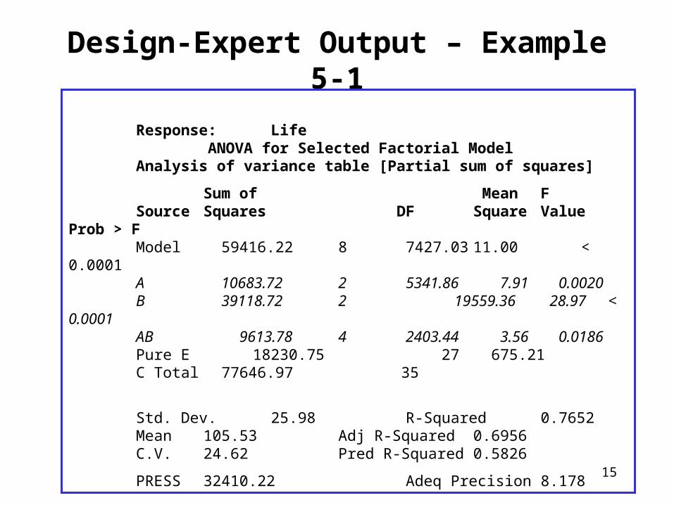
Design-Expert Output – Example 5-1

Response: Life ANOVA for Selected Factorial ModelAnalysis of variance table [Partial sum of squares]

Sum of Mean FSource Squares DF Square Value Prob > FModel 59416.22 8 7427.03 11.00 < 0.0001A 10683.72 2 5341.86 7.91 0.0020B 39118.72 2 19559.36 28.97 < 0.0001AB 9613.78 4 2403.44 3.56 0.0186Pure E 18230.75 27 675.21C Total 77646.97 35

Std. Dev. 25.98 R-Squared 0.7652Mean 105.53 Adj R-Squared 0.6956C.V. 24.62 Pred R-Squared 0.5826

PRESS 32410.22 Adeq Precision 8.178

16

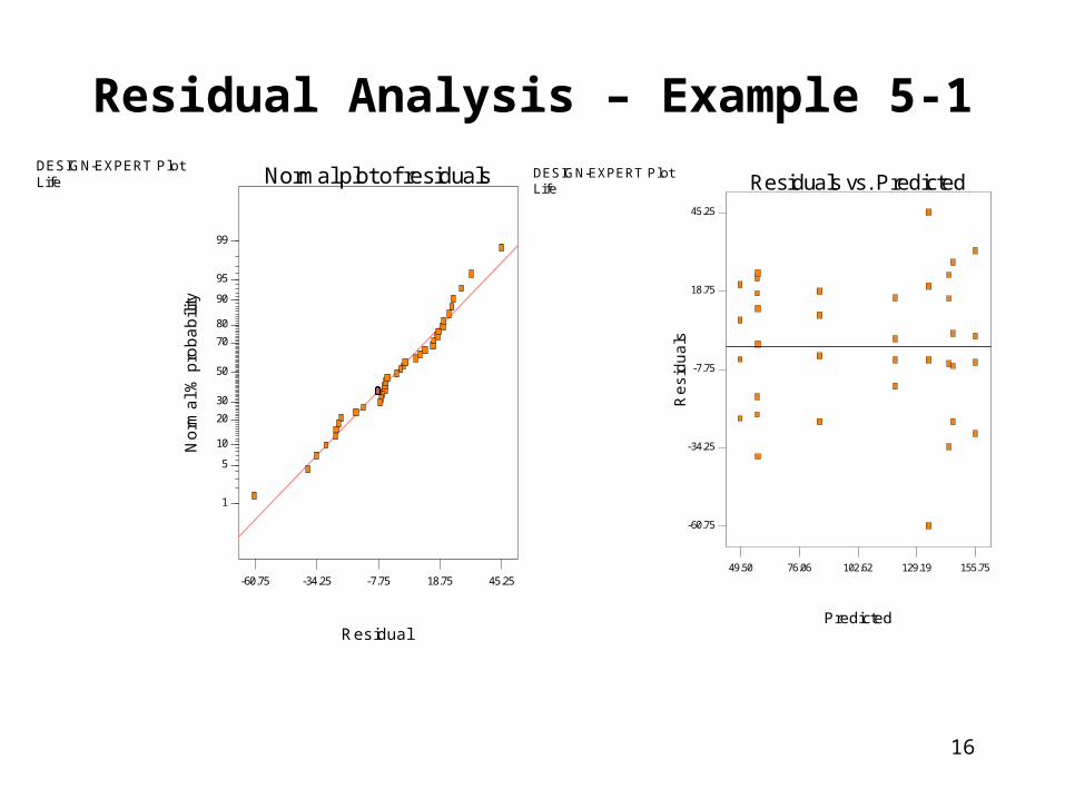
Residual Analysis – Example 5-1DESIGN-EXPERT PlotLife

Residual

No

rma

l % p

rob

ab

ility

Normal plot of residuals

-60.75 -34.25 -7.75 18.75 45.25

1

5

10

20

30

50

70

80

90

95

99

DESIGN-EXPERT PlotLife

Predicted

Re

sid

ua

ls

Residuals vs. Predicted

-60.75

-34.25

-7.75

18.75

45.25

49.50 76.06 102.62 129.19 155.75

17

Residual Analysis – Example 5-1DESIGN-EXPERT PlotLife

Run Number

Re

sid

ua

ls

Residuals vs. Run

-60.75

-34.25

-7.75

18.75

45.25

1 6 11 16 21 26 31 36

18

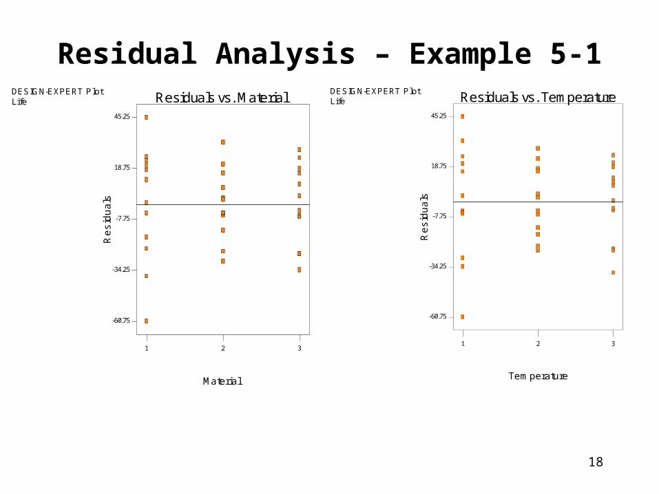
Residual Analysis – Example 5-1DESIGN-EXPERT PlotLife

Material

Re

sid

ua

lsResiduals vs. Material

-60.75

-34.25

-7.75

18.75

45.25

1 2 3

DESIGN-EXPERT PlotLife

Temperature

Re

sid

ua

ls

Residuals vs. Temperature

-60.75

-34.25

-7.75

18.75

45.25

1 2 3

19

Interaction Plot DESIGN-EXPERT Plot

Life

X = B: TemperatureY = A: Material

A1 A1A2 A2A3 A3

A: MaterialInteraction Graph

Life

B: Temperature

15 70 125

20

62

104

146

188

2

2

22

2

2

20

• OC curves can be used to determine sample size (n)• An effective way is to specify a min. diff. between

any two treatment means. E.g. if the difference in any two row means is D, the min. value of 2 is

• If the difference in any two columns is specified,

• If the difference in any two interactions is specified,

Choice of Sample Size

2

22

2 a

nbD

2

22

2 b

naD

]1)1)(1[(2 2

22

ba

nD

21

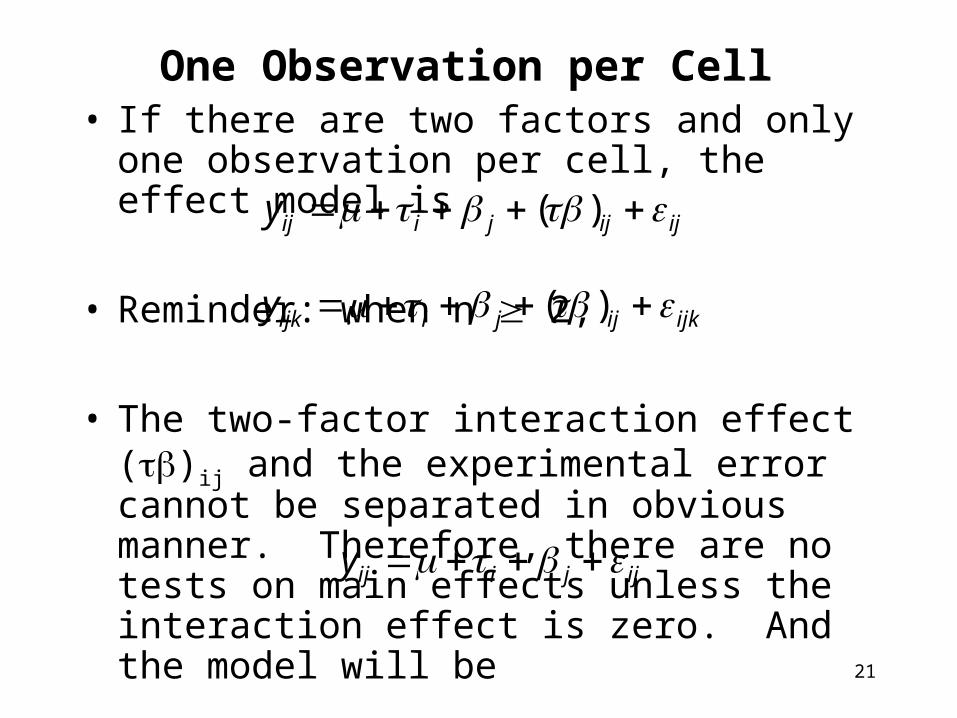
• If there are two factors and only one observation per cell, the effect model is

• Reminder: when n 2,

• The two-factor interaction effect ()ij and the experimental error cannot be separated in obvious manner. Therefore, there are no tests on main effects unless the interaction effect is zero. And the model will be

• The main effects may be tested by comparing MSA and MSB to MSResidual

One Observation per Cell

ijijjiijy )(

ijkijjiijky )(

ijjiijy