1 CSE 326: Data Structures Priority Queues – Binary Heaps.

1

CSE 326: Data Structures

Priority Queues – Binary Heaps

2

Recall Queues

• FIFO: First-In, First-Out

• Some contexts where this seems right?

• Some contexts where some things should be allowed to skip ahead in the line?

3

Queues that Allow Line Jumping

• Need a new ADT

• Operations: Insert an Item, Remove the “Best” Item

insert deleteMin

6 2 15 23 12 18 45 3 7

4

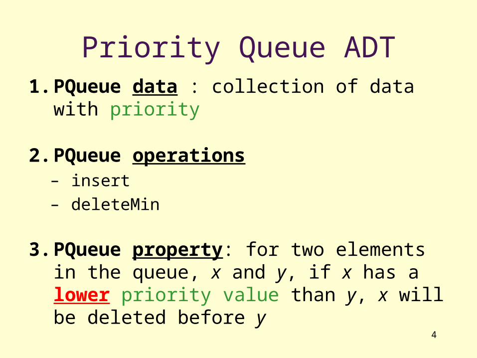
Priority Queue ADT1. PQueue data : collection of data with

priority

2. PQueue operations– insert– deleteMin

3. PQueue property: for two elements in the queue, x and y, if x has a lower priority value than y, x will be deleted before y

5

Applications of the Priority Queue

• Select print jobs in order of decreasing length

• Forward packets on routers in order of urgency

• Select most frequent symbols for compression

• Sort numbers, picking minimum first

• Anything greedy

6

Potential Implementations

insert deleteMin

Unsorted list (Array) O(1) O(n)

Unsorted list (Linked-List) O(1) O(n)

Sorted list (Array) O(n) O(1)*

Sorted list (Linked-List) O(n) O(1)

7

Recall From Lists, Queues, Stacks

• Use an ADT that corresponds to your needs

• The right ADT is efficient, while an overly general ADT provides functionality you aren’t using, but are paying for anyways

• Heaps provide O(log n) worst case for both insert and deleteMin, O(1) average insert

8

Binary Heap Properties

1. Structure Property

2. Ordering Property

9

Tree ReviewA

E

B

D F

C

G

IH

LJ MK N

root(T):

leaves(T):

children(B):

parent(H):

siblings(E):

ancestors(F):

descendents(G):

subtree(C):

Tree T

10

More Tree TerminologyA

E

B

D F

C

G

IH

LJ MK N

depth(B):

height(G):

degree(B):

branching factor(T):

Tree T

11

Brief interlude: Some Definitions:

A Perfect binary tree – A binary tree with all leaf nodes at the same depth. All internal nodes have 2 children.

2592

215

11

307 101 3

16

13 19 22

height h2h+1 – 1 nodes2h – 1 non-leaves2h leaves

12

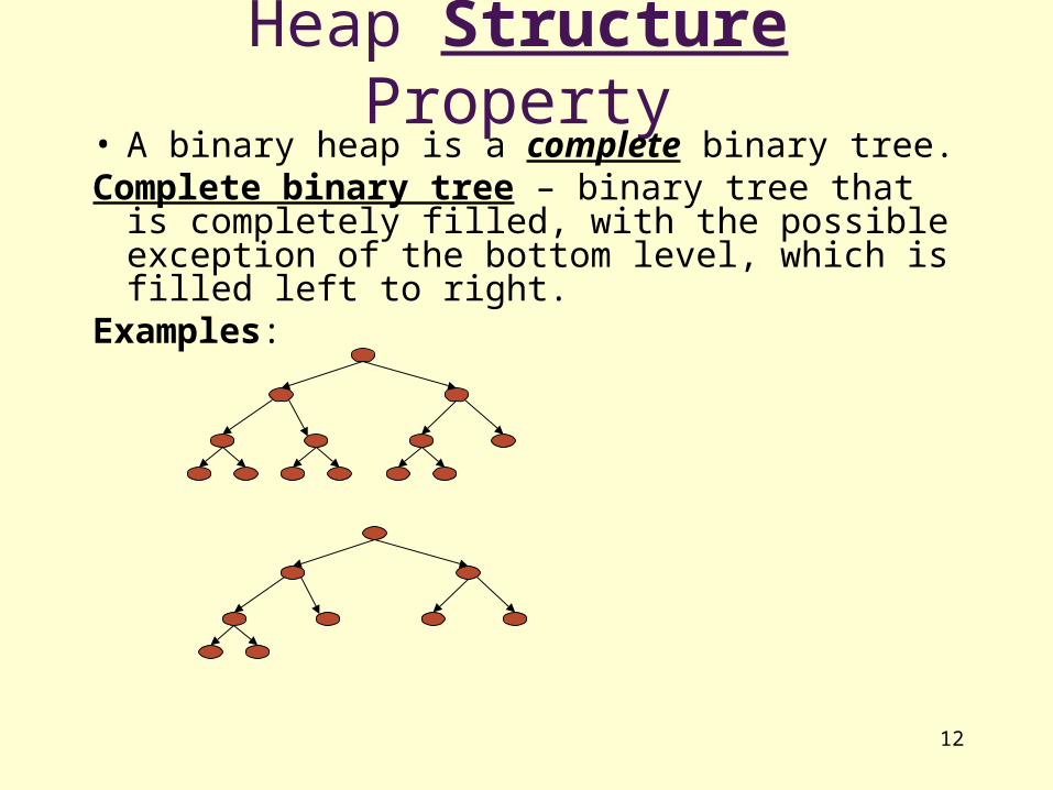
Heap Structure Property• A binary heap is a complete binary tree.Complete binary tree – binary tree that is

completely filled, with the possible exception of the bottom level, which is filled left to right.

Examples:

13

Representing Complete Binary Trees in an Array

GED

CB

A

J KH I

F

L

From node i:

left child:right child:parent:

7

1

2 3

4 5 6

98 10 11 12

A B C D E F G H I J K L

0 1 2 3 4 5 6 7 8 9 10 11 12 13

implicit (array) implementation:

14

Why this approach to storage?

15

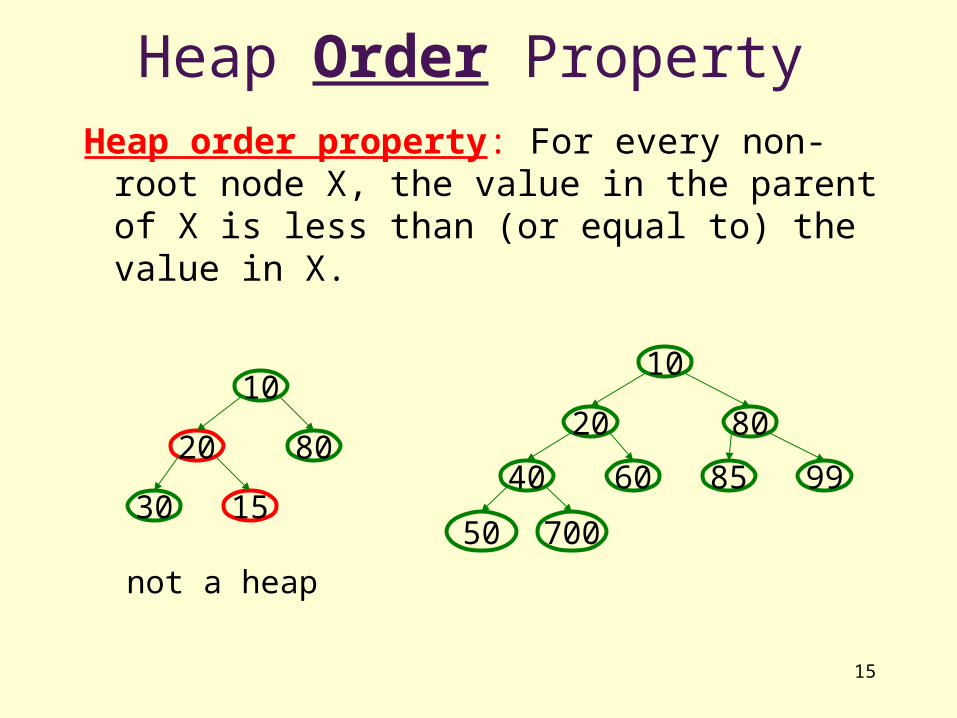
Heap Order Property

Heap order property: For every non-root node X, the value in the parent of X is less than (or equal to) the value in X.

1530

8020

10

996040

8020

10

50 700

85

not a heap

16

Heap Operations• findMin:

• insert(val): percolate up.

• deleteMin: percolate down.

996040

8020

10

50 700

85

65

17

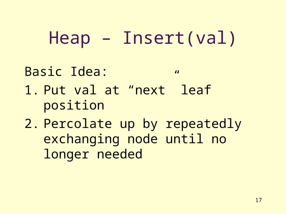
Heap – Insert(val)

Basic Idea:

1. Put val at “next” leaf position

2. Percolate up by repeatedly exchanging node until no longer needed

18

Insert: percolate up

996040

8020

10

50 700

85

65 15

992040

8015

10

50 700

85

65 60

19

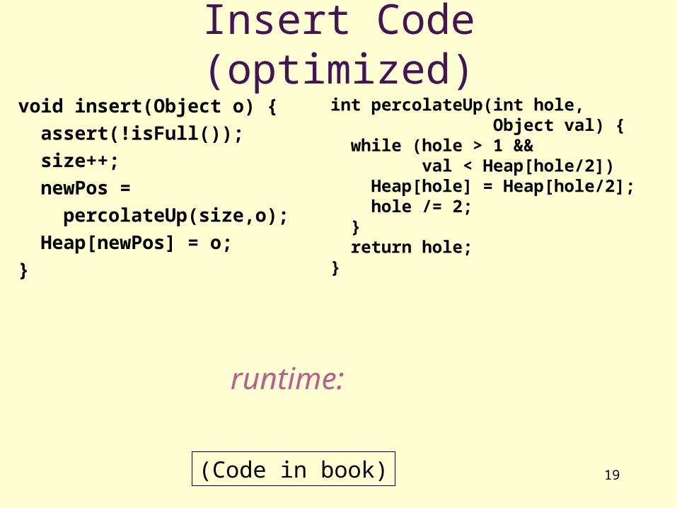
Insert Code (optimized)void insert(Object o) {

assert(!isFull());

size++;

newPos =

percolateUp(size,o);

Heap[newPos] = o;

}

int percolateUp(int hole, Object val) { while (hole > 1 && val < Heap[hole/2]) Heap[hole] = Heap[hole/2]; hole /= 2; } return hole;}

runtime:

(Code in book)

20

Heap – Deletemin

Basic Idea:

1. Remove root (that is always the min!)

2. Put “last” leaf node at root

3. Find smallest child of node

4. Swap node with its smallest child if needed.

5. Repeat steps 3 & 4 until no swaps needed.

21

DeleteMin: percolate down

996040

1520

10

50 700

85

65

996040

6520

15

50 700

85

22

DeleteMin Code (Optimized)

Object deleteMin() {

assert(!isEmpty());

returnVal = Heap[1];

size--;

newPos =

percolateDown(1,

Heap[size+1]);

Heap[newPos] =

Heap[size + 1];

return returnVal;

}

int percolateDown(int hole, Object val) {while (2*hole <= size) { left = 2*hole; right = left + 1; if (right ≤ size && Heap[right] < Heap[left]) target = right; else target = left;

if (Heap[target] < val) { Heap[hole] = Heap[target]; hole = target; } else break; } return hole;}

runtime:

(code in book)

23

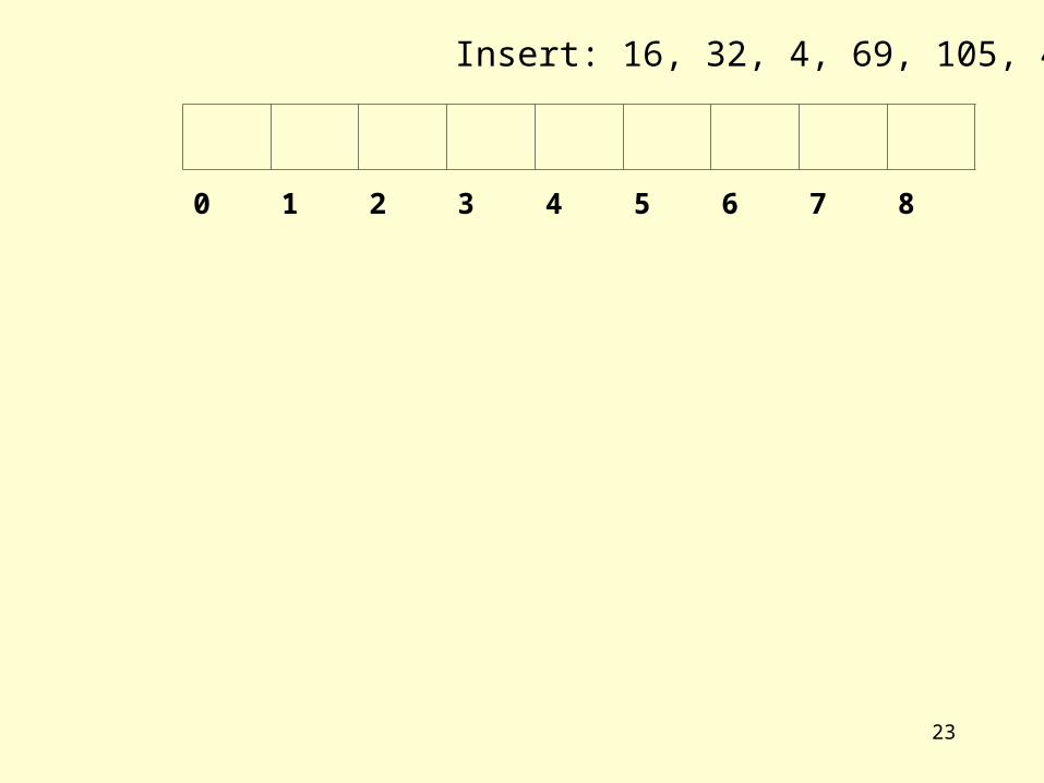
0 1 2 3 4 5 6 7 8

Insert: 16, 32, 4, 69, 105, 43, 2

24

Data Structures

Binary Heaps

25

Building a Heap

5 11 3 10 6 9 4 8 1 7 212

26

Building a Heap

• Adding the items one at a time is O(n log n) in the worst case

• I promised O(n) for today

27

Working on Heaps

• What are the two properties of a heap?– Structure Property– Order Property

• How do we work on heaps?– Fix the structure– Fix the order

28

BuildHeap: Floyd’s Method

5 11 3 10 6 9 4 8 1 7 212

Add elements arbitrarily to form a complete tree.Pretend it’s a heap and fix the heap-order property!

27184

96103

115

12

29

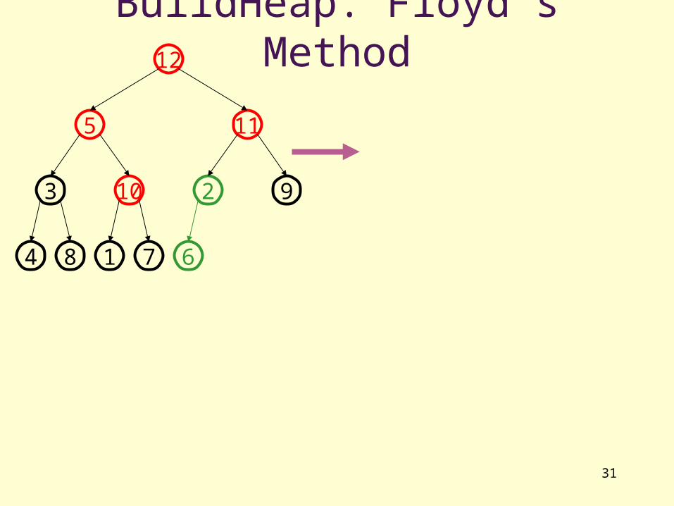
Buildheap pseudocode

private void buildHeap() {

for ( int i = currentSize/2; i > 0; i-- )

percolateDown( i );

}

runtime:

30


27184

96103

115

12

31


67184

92103

115

12

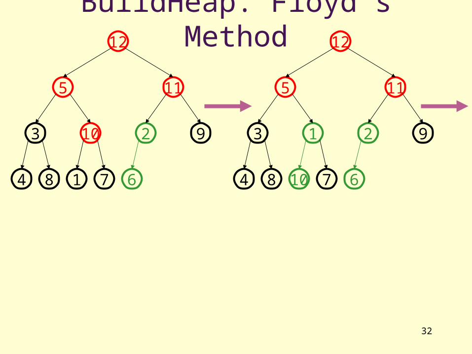
32


67184

92103

115

12

671084

9213

115

12

33


67184

92103

115

12

671084

9213

115

12

1171084

9613

25

12

34


67184

92103

115

12

671084

9213

115

12

1171084

9613

25

12

1171084

9653

21

12

35

Finally…

11710812

9654

23

1

runtime:

36

More Priority Queue Operations• decreaseKey

– given a pointer to an object in the queue, reduce its priority value

Solution: change priority and ____________________________

• increaseKey– given a pointer to an object in the queue, increase its priority value

Solution: change priority and _____________________________

Why do we need a pointer? Why not simply data value?

37

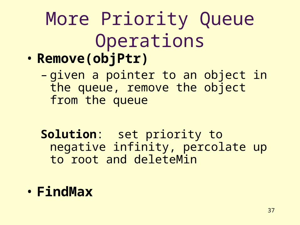
More Priority Queue Operations

• Remove(objPtr)– given a pointer to an object in the queue,

remove the object from the queue

Solution: set priority to negative infinity, percolate up to root and deleteMin

• FindMax

38

Facts about HeapsObservations:• Finding a child/parent index is a multiply/divide by two

• Operations jump widely through the heap

• Each percolate step looks at only two new nodes

• Inserts are at least as common as deleteMins

Realities:• Division/multiplication by powers of two are equally fast

• Looking at only two new pieces of data: bad for cache!

• With huge data sets, disk accesses dominate

39

CPU

Cache

Memory

Disk

Cycles to access:

40

4

9654

23

1

8 1012

7

11

A Solution: d-Heaps• Each node has d

children• Still representable by

array• Good choices for d:

– (choose a power of two for efficiency)

– fit one set of children in a cache line

– fit one set of children on a memory page/disk block

3 7 2 8 5 12 11 10 6 9112

41

One More Operation

• Merge two heaps

• Add the items from one into another?– O(n log n)

• Start over and build it from scratch?– O(n)

42

CSE 326: Data Structures

Priority Queues Leftist Heaps & Skew Heaps

43

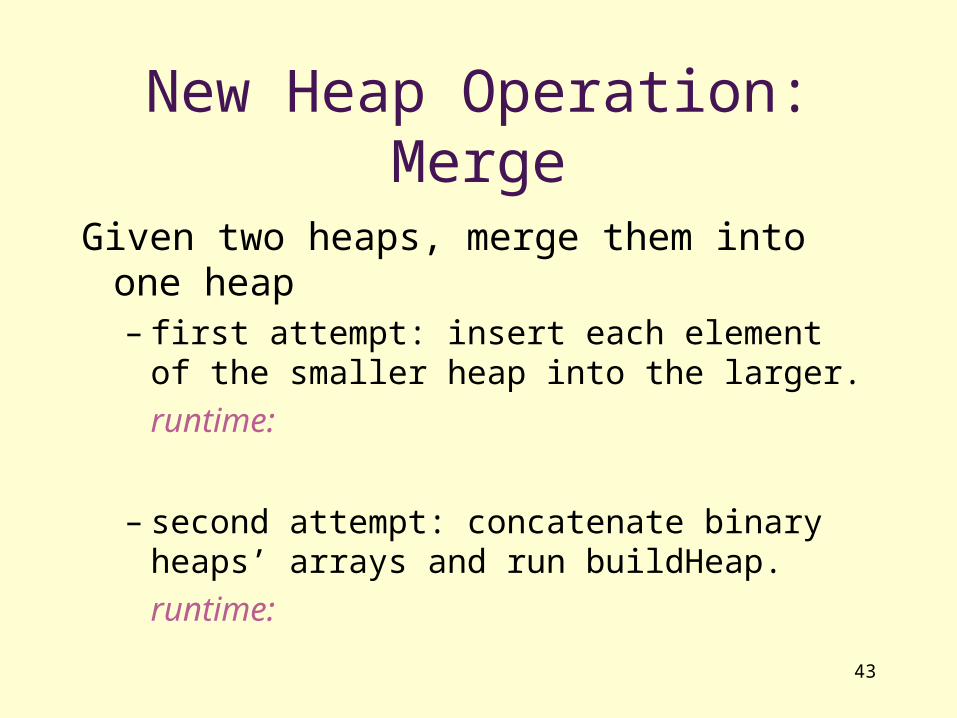
New Heap Operation: Merge

Given two heaps, merge them into one heap– first attempt: insert each element of the

smaller heap into the larger.

runtime:

– second attempt: concatenate binary heaps’ arrays and run buildHeap.

runtime:

44

Leftist Heaps

Idea:

Focus all heap maintenance work in one small part of the heap

Leftist heaps:1. Most nodes are on the left

2. All the merging work is done on the right

45

null path length (npl) of a node x = the number of nodes between x and a null in its subtree

ORnpl(x) = min distance to a descendant with 0 or 1 children

Definition: Null Path Length

• npl(null) = -1• npl(leaf) = 0• npl(single-child node) = 0

000

0?1

??

?

Equivalent definitions:

1. npl(x) is the height of largest complete subtree rooted at x

2. npl(x) = 1 + min{npl(left(x)), npl(right(x))}

0

46

Leftist Heap Properties• Heap-order property

– parent’s priority value is to childrens’ priority values– result: minimum element is at the root

• Leftist property– For every node x, npl(left(x)) npl(right(x))– result: tree is at least as “heavy” on the left as the

right

47

Are These Leftist?

00

001

11

2

0

0

000

11

2

1

000

0

0

0

0

0

1

0 0

Every subtree of a leftist tree is leftist!

48

Right Path in a Leftist Tree is Short (#1)

Claim: The right path is as short as any in the tree.Proof: (By contradiction)

R

x

LD2

D1

Pick a shorter path: D1 < D2

Say it diverges from right path at x

npl(L) D1-1 because of the path of

length D1-1 to null

npl(R) D2-1 because every node on right path is leftistLeftist property at x violated!

49

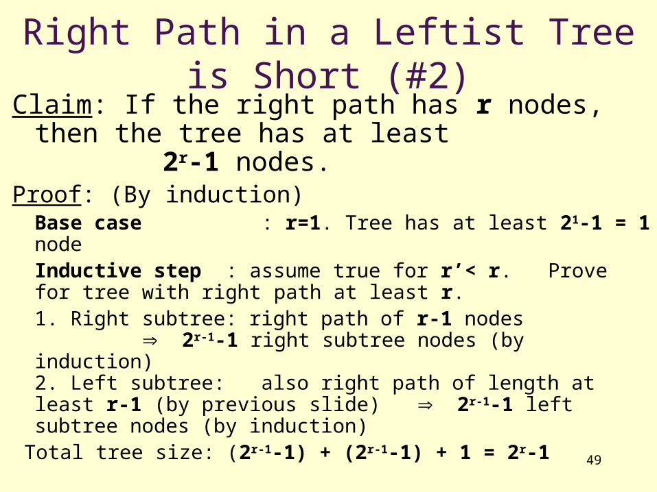
Right Path in a Leftist Tree is Short (#2)Claim: If the right path has r nodes, then the tree

has at least 2r-1 nodes.

Proof: (By induction)Base case : r=1. Tree has at least 21-1 = 1 nodeInductive step : assume true for r’< r. Prove for tree with right path at least r.1. Right subtree: right path of r-1 nodes

2r-1-1 right subtree nodes (by induction)2. Left subtree: also right path of length at least r-1 (by previous slide) 2r-1-1 left subtree nodes (by induction)

Total tree size: (2r-1-1) + (2r-1-1) + 1 = 2r-1

50

Why do we have the leftist property?

Because it guarantees that:

• the right path is really short compared to the number of nodes in the tree

• A leftist tree of N nodes, has a right path of at most lg (N+1) nodes

Idea – perform all work on the right path

51

Merge two heaps (basic idea)

• Put the smaller root as the new root,

• Hang its left subtree on the left.

• Recursively merge its right subtree and the other tree.

52

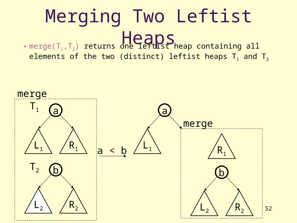
Merging Two Leftist Heaps• merge(T1,T2) returns one leftist heap containing all

elements of the two (distinct) leftist heaps T1 and T2

a

L1 R1

b

L2 R2

mergeT1

T2

a < b

a

L1

merge

b

L2 R2

R1

53

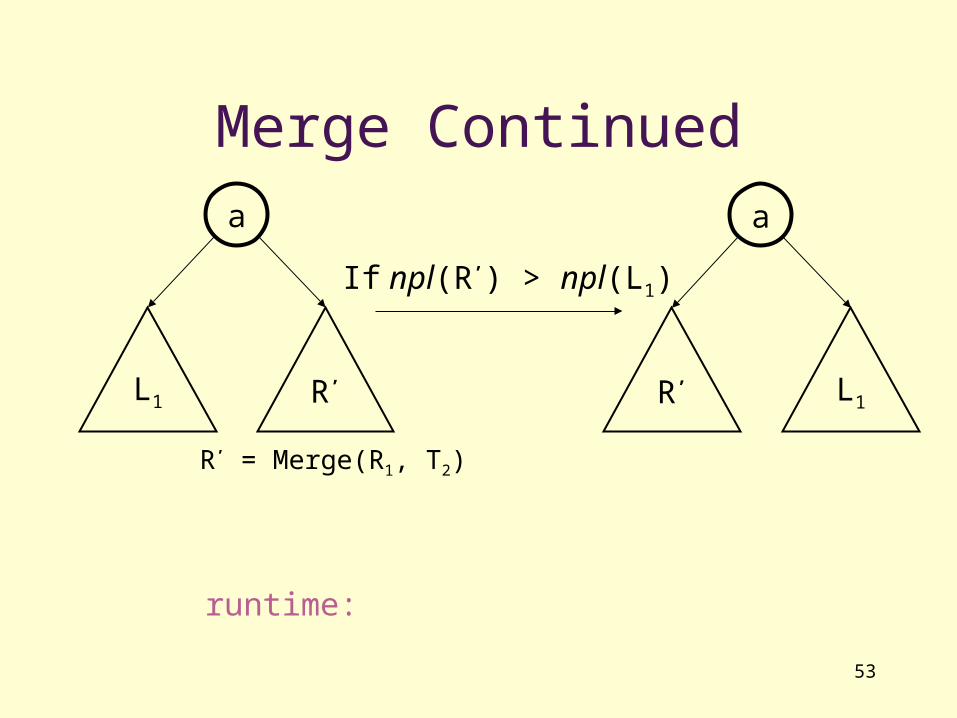
Merge Continueda

L1 R’

R’ = Merge(R1, T2)

a

R’ L1

If npl(R’) > npl(L1)

runtime:

54

Let’s do an example, but first…Other Heap Operations

• insert ?

• deleteMin ?

55

Operations on Leftist Heaps• merge with two trees of total size n: O(log n)• insert with heap size n: O(log n)

– pretend node is a size 1 leftist heap– insert by merging original heap with one node

heap

• deleteMin with heap size n: O(log n)– remove and return root– merge left and right subtrees

merge

merge

56

Leftest Merge Example

1210

5

87

3

14

1

0 0

1

0 0

0

merge

7

3

14

?

0

0

1210

5

8

1

0 0

0

merge

10

5?

0 merge

12

8

0

0

8

12

0

0

(special case)

57

Sewing Up the Example

8

12

0

0

10

5?

0

7

3

14

?

0

0

8

12

0

0

10

51

0

7

3

14

?

0

08

12

0

0

10

5 1

0

7

3

14

1

0

0

Done?

58

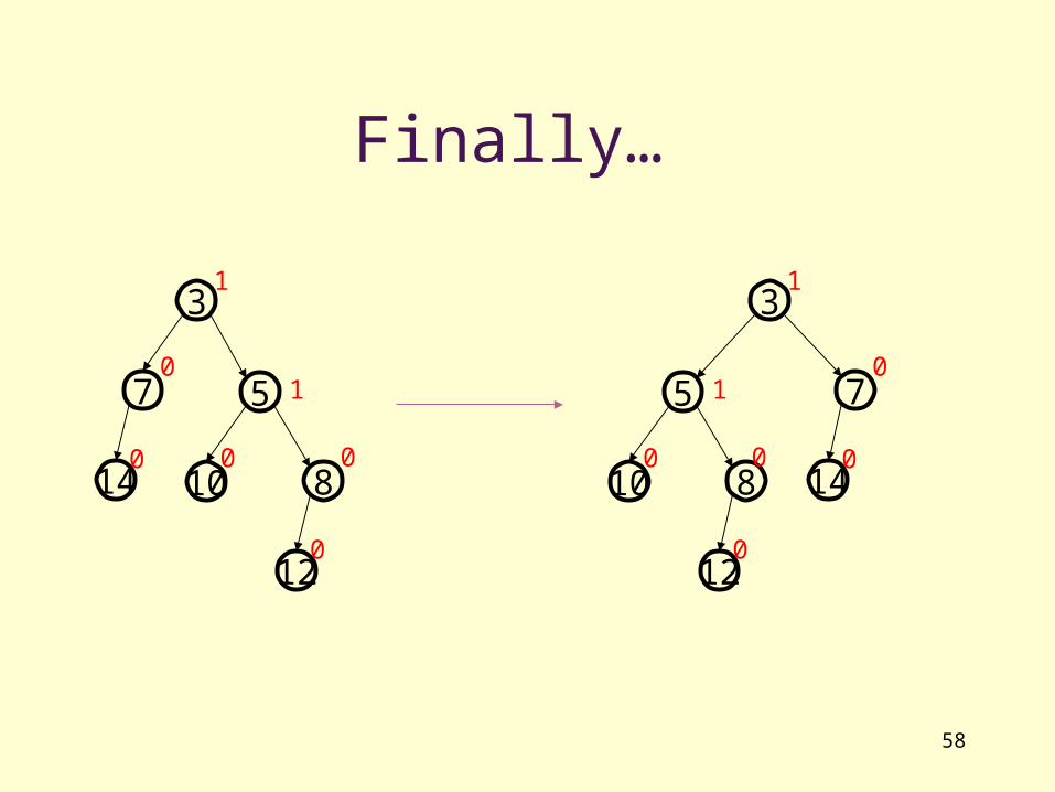
Finally…

8

12

0

0

10

5 1

0

7

3

14

1

0

0

7

3

14

1

0

08

12

0

0

10

5 1

0

59

Leftist Heaps: Summary

Good

•

•

Bad

•

•

60

Random Definition:Amortized Time

am·or·tized time: Running time limit resulting from “writing off” expensive runs of an algorithm over multiple cheap runs of the algorithm, usually resulting in a lower overall running time than indicated by the worst possible case.

If M operations take total O(M log N) time, amortized time per operation is O(log N)

Difference from average time:

61

Skew HeapsProblems with leftist heaps

– extra storage for npl– extra complexity/logic to maintain and check npl – right side is “often” heavy and requires a switch

Solution: skew heaps– “blindly” adjusting version of leftist heaps– merge always switches children when fixing right

path– amortized time for: merge, insert, deleteMin = O(log

n)– however, worst case time for all three = O(n)

62

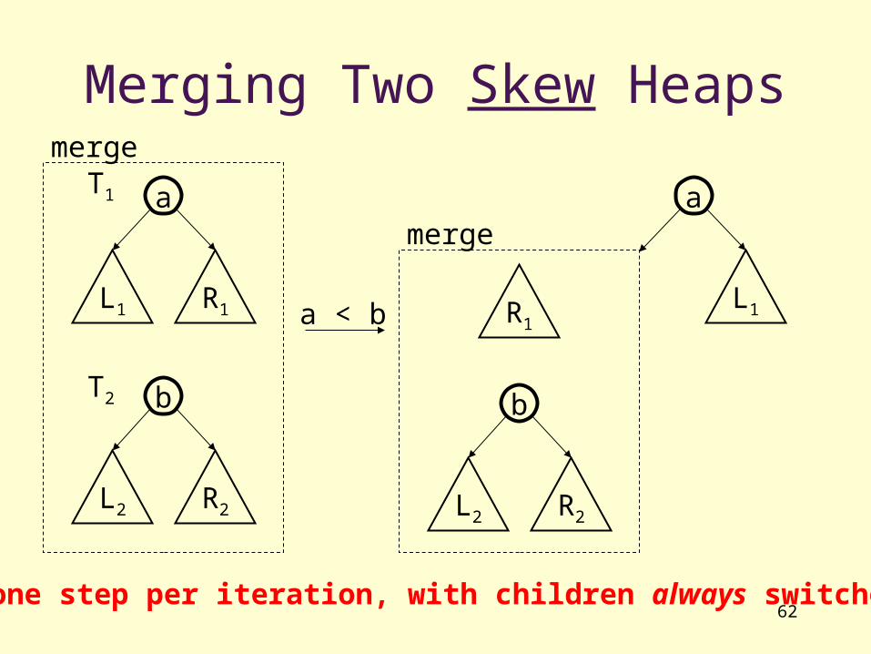
Merging Two Skew Heaps

a

L1 R1

b

L2 R2

mergeT1

T2

a < b

a

L1

merge

b

L2 R2

R1

Only one step per iteration, with children always switched

63

Example

1210

5

87

3

14

merge

7

3

141210

5

8

merge7

3

1410

5

8

merge12

7

3

14108

5

12

64

Skew Heap Codevoid merge(heap1, heap2) {

case {

heap1 == NULL: return heap2;

heap2 == NULL: return heap1;

heap1.findMin() < heap2.findMin():

temp = heap1.right;

heap1.right = heap1.left;

heap1.left = merge(heap2, temp);

return heap1;

otherwise:

return merge(heap2, heap1);

}

}

65

Runtime Analysis:Worst-case and Amortized

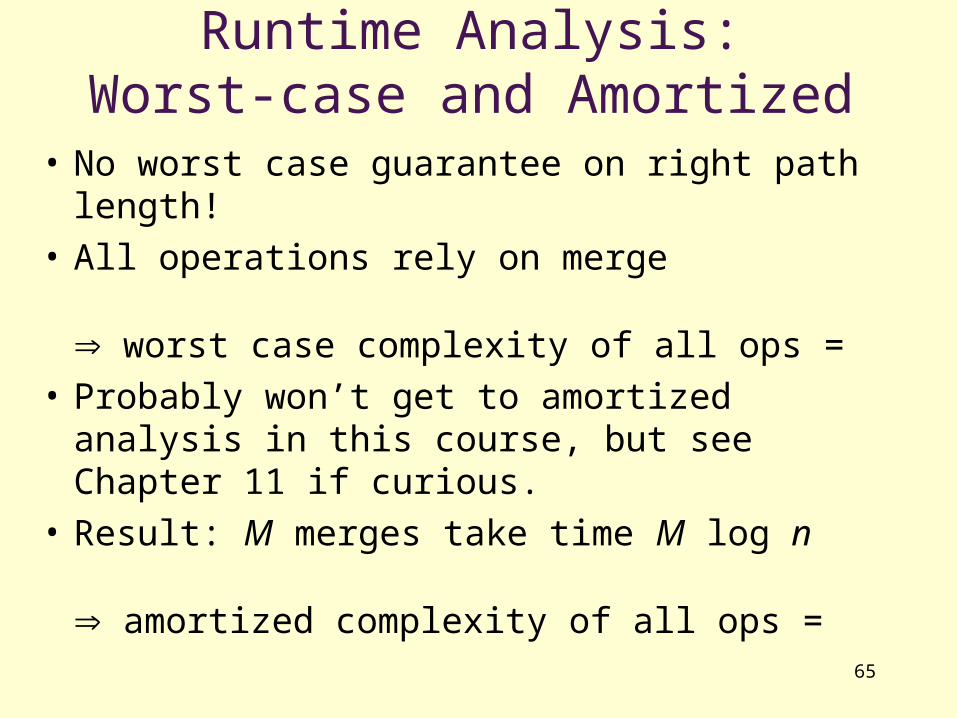
• No worst case guarantee on right path length!

• All operations rely on merge

worst case complexity of all ops =

• Probably won’t get to amortized analysis in this course, but see Chapter 11 if curious.

• Result: M merges take time M log n

amortized complexity of all ops =

66

Comparing Heaps

• Binary Heaps

• d-Heaps

• Leftist Heaps

• Skew Heaps

Still room for improvement! (Where?)

Data StructuresBinomial Queues

67

Yet Another Data Structure:Binomial Queues

• Structural property– Forest of binomial trees with at most

one tree of any height

• Order property– Each binomial tree has the heap-order

property

68

What’s a forest?

What’s a binomial tree?

The Binomial Tree, Bh• Bh has height h and exactly 2h nodes• Bh is formed by making Bh-1 a child of another Bh-1

• Root has exactly h children• Number of nodes at depth d is binomial coeff.

– Hence the name; we will not use this last property

d

h

69

B0 B1 B2 B3

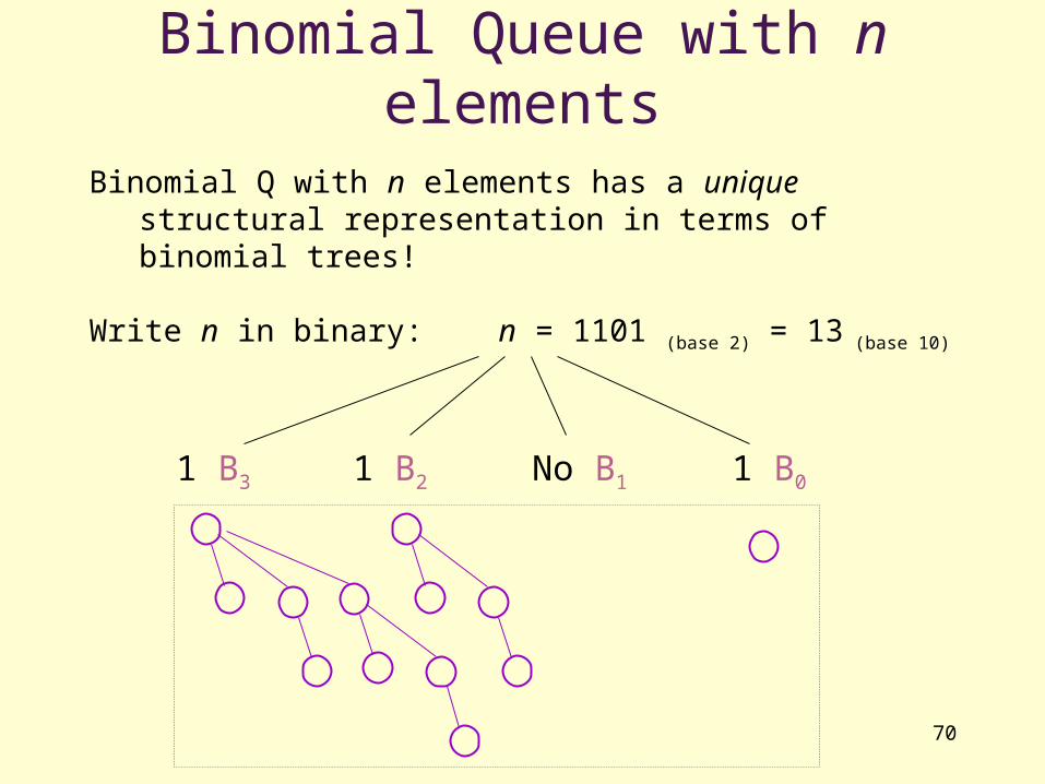
Binomial Queue with n elements

Binomial Q with n elements has a unique structural representation in terms of binomial trees!

Write n in binary: n = 1101 (base 2) = 13 (base 10)

70

1 B3 1 B2 No B1 1 B0

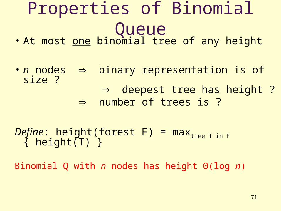
Properties of Binomial Queue• At most one binomial tree of any height

• n nodes binary representation is of size ? deepest tree has height ? number of trees is ?

Define: height(forest F) = maxtree T in F { height(T) }

Binomial Q with n nodes has height Θ(log n)

71

Operations on Binomial Queue

• Will again define merge as the base operation– insert, deleteMin, buildBinomialQ will use merge

• Can we do increaseKey efficiently?decreaseKey?

• What about findMin?

72

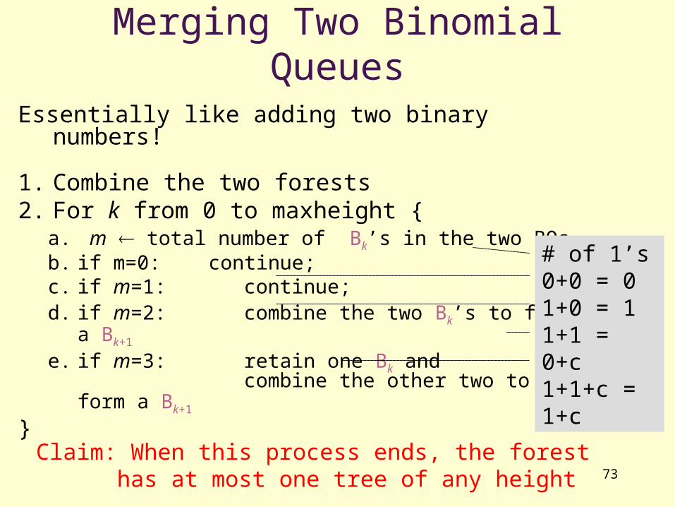
Merging Two Binomial Queues

Essentially like adding two binary numbers!

1. Combine the two forests2. For k from 0 to maxheight {

a. m total number of Bk’s in the two BQsb. if m=0: continue;c. if m=1: continue;d. if m=2: combine the two Bk’s to form a

Bk+1

e. if m=3: retain one Bk and combine the other two to form a

Bk+1

}73

Claim: When this process ends, the forest has at most one tree of any height

# of 1’s0+0 = 01+0 = 11+1 = 0+c1+1+c = 1+c

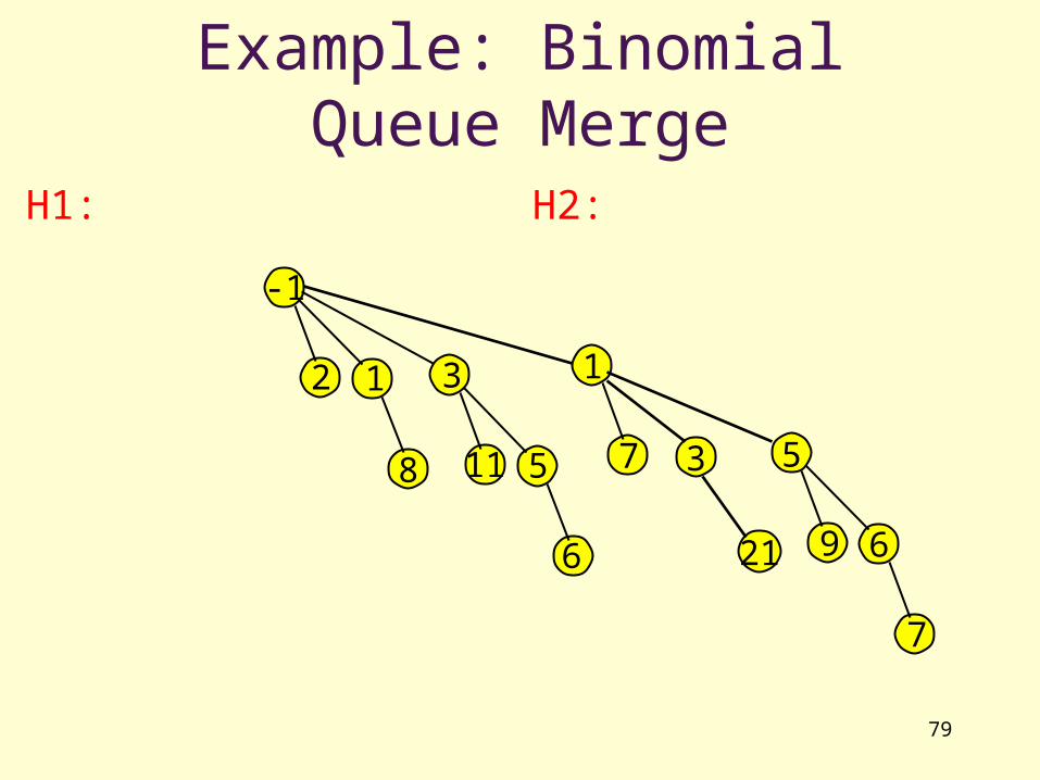
Example: Binomial Queue Merge

74

31

7

-1

2 1 3

8 11 5

6

5

9 6

7

21

H1: H2:


75

31

7

-1

2 1 3

8 11 5

6

5

9 6

7

21

H1: H2:


76

3

1

7

-1

2 1 3

8 11 5

6

5

9 6

721

H1: H2:


77

3

1

7

-1

2 1 3

8 11 5

6

5

9 6

7

21

H1: H2:


78

3

1

7

-1

2 1 3

8 11 5

6

5

9 6

7

21

H1: H2:


79

3

1

7

-1

2 1 3

8 11 5

6

5

9 6

7

21

H1: H2:

Complexity of Merge

Constant time for each height

Max number of heights is: log n

worst case running time = Θ( )

80

Insert in a Binomial Queue

Insert(x): Similar to leftist or skew heap

runtime

Worst case complexity: same as merge O( )

Average case complexity: O(1)

Why?? Hint: Think of adding 1 to 1101

81

deleteMin in Binomial QueueSimilar to leftist and skew heaps….

82

deleteMin: Example

83

4

8

3

7

5

7BQ

8

7

5

find and deletesmallest root merge BQ

(without

the shaded part) and BQ’

BQ’

deleteMin: Example

84

8

4

7

5

7Result:

runtime:

1 CSE 326: Data Structures Priority Queues – Binary Heaps.

Documents

Transcript of 1 CSE 326: Data Structures Priority Queues – Binary Heaps.