
1 CSC 463 Fall 2010 Dr. Adam P. Anthony Class #27.
62
1 CSC 463 Fall 2010 Dr. Adam P. Anthony Class #27
-
Upload
michaela-loveday -
Category
Documents
-
view
216 -
download
0
Transcript of 1 CSC 463 Fall 2010 Dr. Adam P. Anthony Class #27.

1
CSC 463Fall 2010
Dr. Adam P. Anthony
Class #27
2
Machine Learning III
Chapter 18.9

3
Today’s class
• Support vector machines• Clustering (unsupervised learning)

Support Vector Machines
4
These SVM slides were borrowed from Andrew Moore’s PowetPoint slides on SVMs. Andrew’s PowerPoint repository is here:http://www.cs.cmu.edu/~awm/tutorials . Comments and corrections gratefully received.

5
Methods For Classification
• Decision Trees– Model-based data structure, works best with discrete data– For a new instance, choose label C based on rules laid out by tree
• Probabilistic Classifiers– Model-based as well, works with any type of data– For a new instance, choose label C that maximizes
P([f1…fn,C] | Data)
• K-Nearest Neighbor– Instance-based– For new instance, choose label based on the majority vote of k nearest points in Data
• Boundary-Based Classifiers (NEW!)– Model-based, only works with continuous data– Establish a numerical function that acts as a fence between positive, negative examples
Copyright © 2001, 2003, Andrew W. Moore
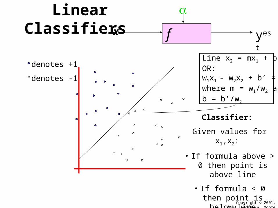
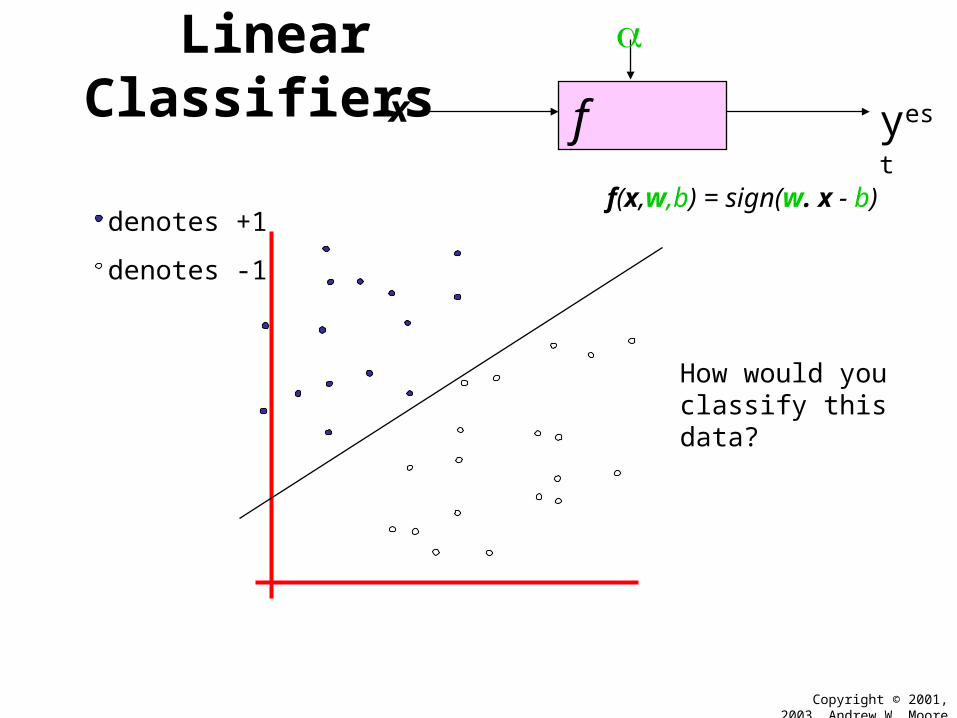
Linear Classifiersf x
yest
denotes +1
denotes -1
Classifier:
Given values for x1,x2:
• If formula above > 0 then point is above line
• If formula < 0 then point is below line
f(x,w,b) = sign(w. x + b)
Line x2 = mx1 + bOR: w1x1 - w2x2 + b’ = 0where m = w1/w2 and b = b’/w2
Copyright © 2001, 2003, Andrew W. Moore
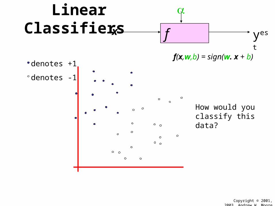
Linear Classifiersf x
yest
denotes +1
denotes -1
f(x,w,b) = sign(w. x + b)
How would you classify this data?
Copyright © 2001, 2003, Andrew W. Moore
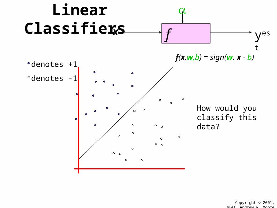
Linear Classifiersf x
yest
denotes +1
denotes -1
f(x,w,b) = sign(w. x - b)
How would you classify this data?
Copyright © 2001, 2003, Andrew W. Moore
Linear Classifiersf x
yest
denotes +1
denotes -1
f(x,w,b) = sign(w. x - b)
How would you classify this data?

Copyright © 2001, 2003, Andrew W. Moore
Linear Classifiersf x
yest
denotes +1
denotes -1
f(x,w,b) = sign(w. x - b)
How would you classify this data?
Copyright © 2001, 2003, Andrew W. Moore
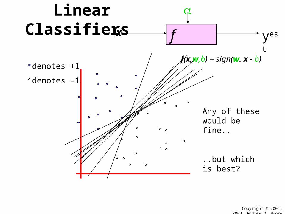
Linear Classifiersf x
yest
denotes +1
denotes -1
f(x,w,b) = sign(w. x - b)
Any of these would be fine..
..but which is best?
Copyright © 2001, 2003, Andrew W. Moore
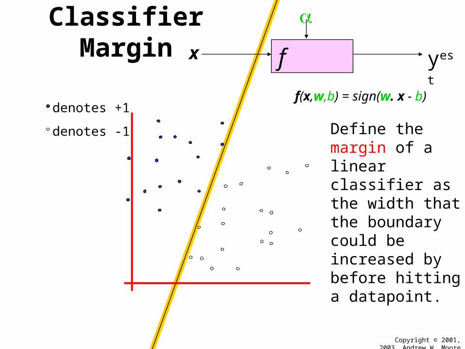
Classifier Marginf x
yest
denotes +1
denotes -1
f(x,w,b) = sign(w. x - b)
Define the margin of a linear classifier as the width that the boundary could be increased by before hitting a datapoint.

Copyright © 2001, 2003, Andrew W. Moore
Maximum Marginf x
yest
denotes +1
denotes -1
f(x,w,b) = sign(w. x - b)
The maximum margin linear classifier is the linear classifier with the, um, maximum margin.
This is the simplest kind of SVM (Called an LSVM)
Linear SVM

Copyright © 2001, 2003, Andrew W. Moore
Maximum Marginf x
yest
denotes +1
denotes -1
f(x,w,b) = sign(w. x - b)
The maximum margin linear classifier is the linear classifier with the, um, maximum margin.
This is the simplest kind of SVM (Called an LSVM)
Support Vectors are those datapoints that the margin pushes up against
Linear SVM
Copyright © 2001, 2003, Andrew W. Moore
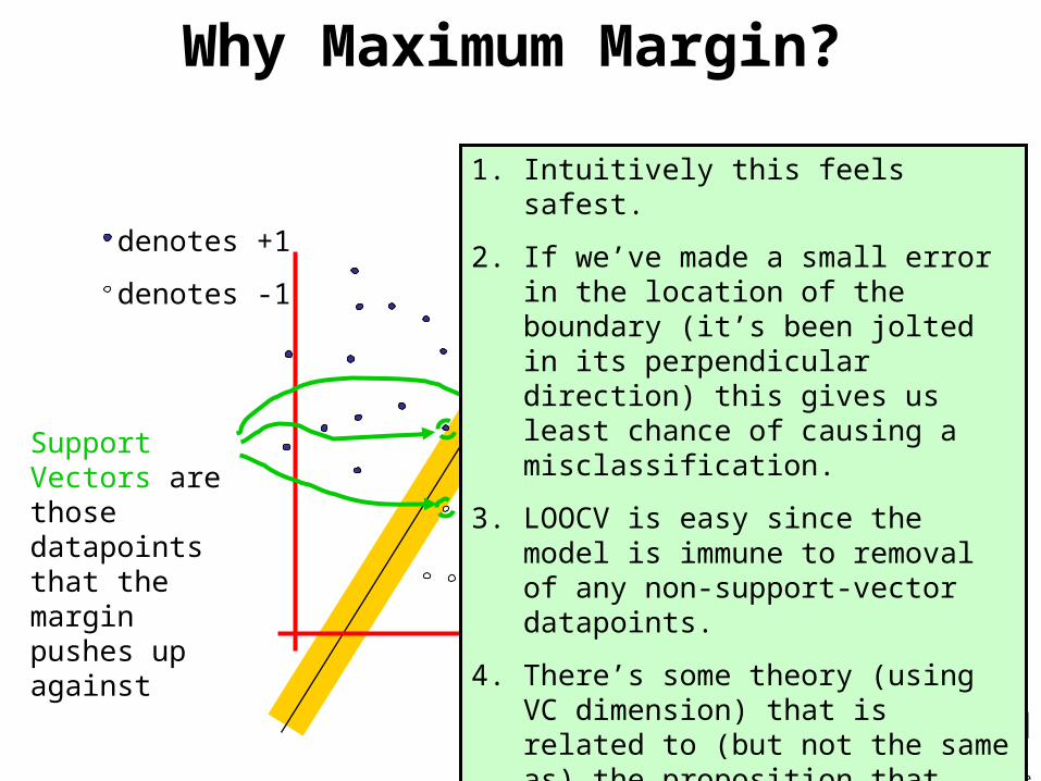
Why Maximum Margin?
denotes +1
denotes -1
f(x,w,b) = sign(w. x - b)
The maximum margin linear classifier is the linear classifier with the, um, maximum margin.
This is the simplest kind of SVM (Called an LSVM)
Support Vectors are those datapoints that the margin pushes up against
1. Intuitively this feels safest.
2. If we’ve made a small error in the location of the boundary (it’s been jolted in its perpendicular direction) this gives us least chance of causing a misclassification.
3. LOOCV is easy since the model is immune to removal of any non-support-vector datapoints.
4. There’s some theory (using VC dimension) that is related to (but not the same as) the proposition that this is a good thing.
5. Empirically it works very very well.

Copyright © 2001, 2003, Andrew W. Moore
Specifying a line and margin
• How do we represent this mathematically?• …in m input dimensions?
Plus-Plane
Minus-Plane
Classifier Boundary
“Predict Class = +1” zone
“Predict Class = -1” zone

Copyright © 2001, 2003, Andrew W. Moore
Specifying a line and margin
• Plus-plane = { x : w . x + b = +1 }• Minus-plane = { x : w . x + b = -1 }
Plus-Plane
Minus-Plane
Classifier Boundary
“Predict Class = +1” zone
“Predict Class = -1” zone
Classify as..
+1 if w . x + b >= 1
-1 if w . x + b <= -1
Universe explodes
if -1 < w . x + b < 1
wx+b=1
wx+b=0
wx+b=-1
Copyright © 2001, 2003, Andrew W. Moore
Computing the margin width
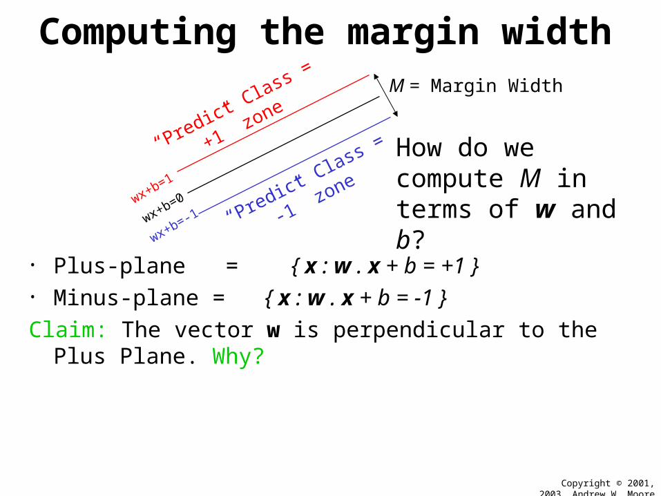
• Plus-plane = { x : w . x + b = +1 }• Minus-plane = { x : w . x + b = -1 }
Claim: The vector w is perpendicular to the Plus Plane. Why?
“Predict Class = +1” zone
“Predict Class = -1” zone
wx+b=1
wx+b=0
wx+b=-1
M = Margin Width
How do we compute M in terms of w and b?
Copyright © 2001, 2003, Andrew W. Moore
Computing the margin width
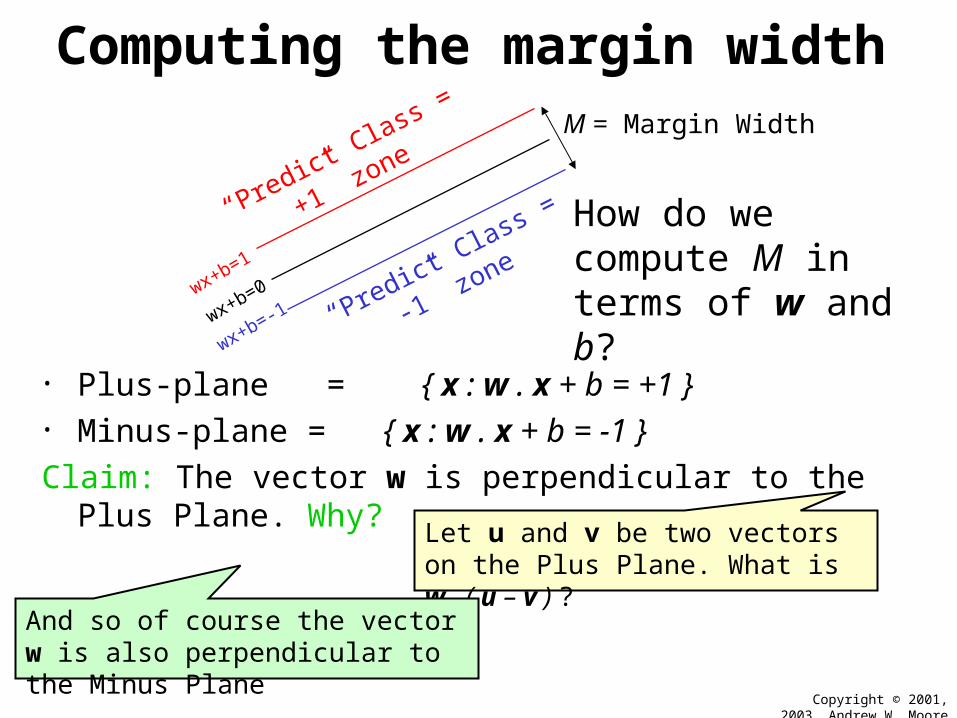
• Plus-plane = { x : w . x + b = +1 }• Minus-plane = { x : w . x + b = -1 }
Claim: The vector w is perpendicular to the Plus Plane. Why?
“Predict Class = +1” zone
“Predict Class = -1” zone
wx+b=1
wx+b=0
wx+b=-1
M = Margin Width
How do we compute M in terms of w and b?
Let u and v be two vectors on the Plus Plane. What is w . ( u – v ) ?
And so of course the vector w is also perpendicular to the Minus Plane
Copyright © 2001, 2003, Andrew W. Moore
Computing the margin width
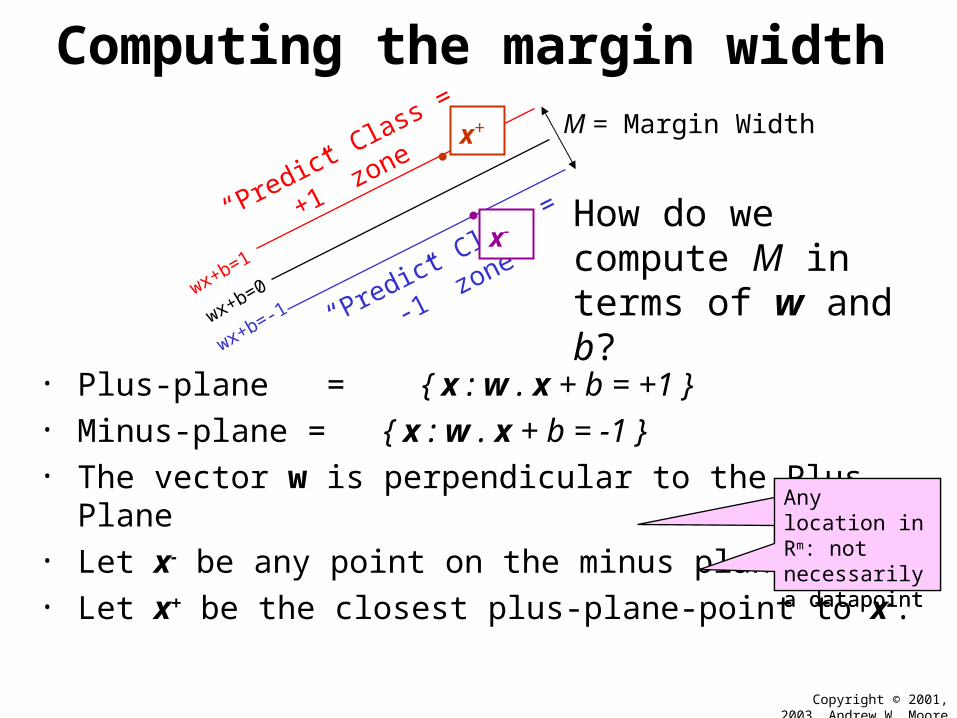
• Plus-plane = { x : w . x + b = +1 }• Minus-plane = { x : w . x + b = -1 }• The vector w is perpendicular to the Plus Plane• Let x- be any point on the minus plane• Let x+ be the closest plus-plane-point to x-.
“Predict Class = +1” zone
“Predict Class = -1” zone
wx+b=1
wx+b=0
wx+b=-1
M = Margin Width
How do we compute M in terms of w and b?
x-
x+
Any location in m: not necessarily a datapoint
Any location in Rm: not necessarily a datapoint
Copyright © 2001, 2003, Andrew W. Moore
Computing the margin width
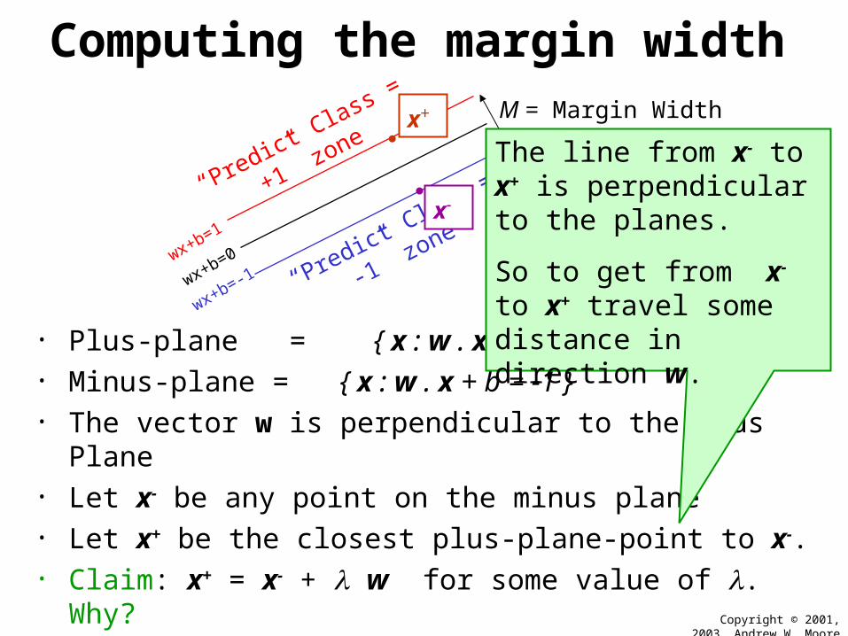
• Plus-plane = { x : w . x + b = +1 }• Minus-plane = { x : w . x + b = -1 }• The vector w is perpendicular to the Plus Plane• Let x- be any point on the minus plane• Let x+ be the closest plus-plane-point to x-.• Claim: x+ = x- + w for some value of . Why?
“Predict Class = +1” zone
“Predict Class = -1” zone
wx+b=1
wx+b=0
wx+b=-1
M = Margin Width
How do we compute M in terms of w and b?
x-
x+
Copyright © 2001, 2003, Andrew W. Moore
Computing the margin width
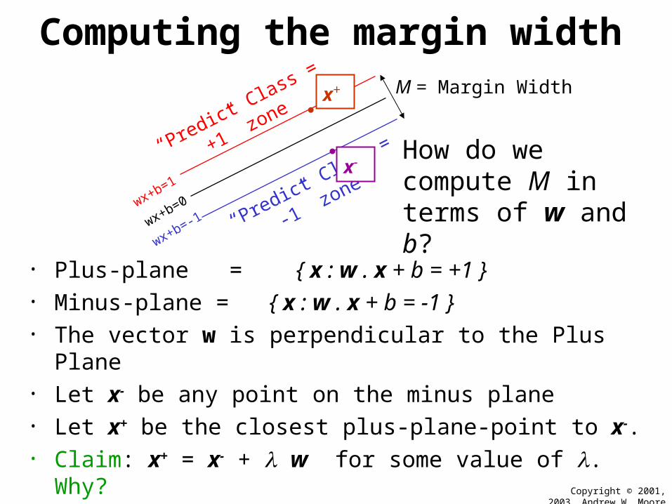
• Plus-plane = { x : w . x + b = +1 }• Minus-plane = { x : w . x + b = -1 }• The vector w is perpendicular to the Plus Plane• Let x- be any point on the minus plane• Let x+ be the closest plus-plane-point to x-.• Claim: x+ = x- + w for some value of . Why?
“Predict Class = +1” zone
“Predict Class = -1” zone
wx+b=1
wx+b=0
wx+b=-1
M = Margin Width
How do we compute M in terms of w and b?
x-
x+
The line from x- to x+ is perpendicular to the planes.
So to get from x- to x+ travel some distance in direction w.
Copyright © 2001, 2003, Andrew W. Moore
Computing the margin width
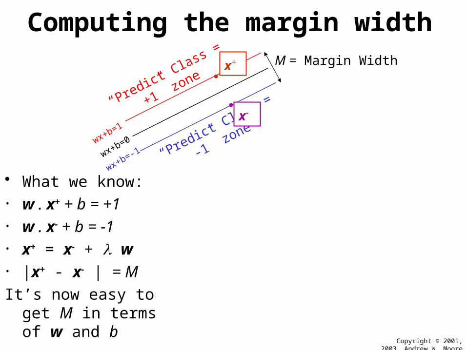
• What we know:• w . x+ + b = +1 • w . x- + b = -1 • x+ = x- + w• |x+ - x- | = M
It’s now easy to get M in terms of w and b
“Predict Class = +1” zone
“Predict Class = -1” zone
wx+b=1
wx+b=0
wx+b=-1
M = Margin Width
x-
x+
Copyright © 2001, 2003, Andrew W. Moore
Computing the margin width
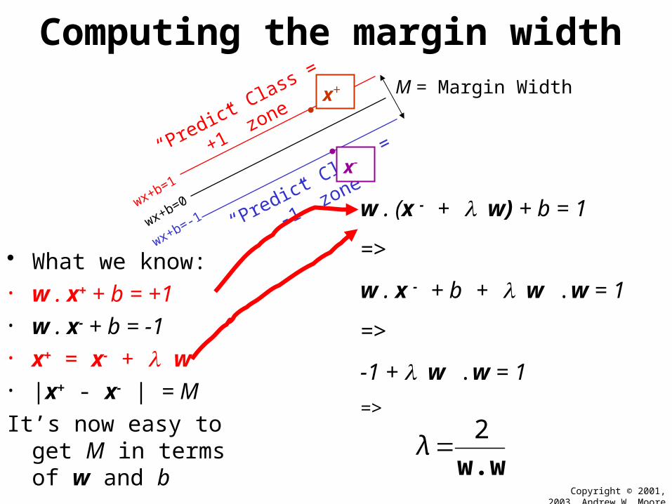
• What we know:• w . x+ + b = +1 • w . x- + b = -1 • x+ = x- + w• |x+ - x- | = M
It’s now easy to get M in terms of w and b
“Predict Class = +1” zone
“Predict Class = -1” zone
wx+b=1
wx+b=0
wx+b=-1
M = Margin Width
w . (x - + w) + b = 1
=>
w . x - + b + w .w = 1
=>
-1 + w .w = 1
=>
x-
x+
w.w
2λ
Copyright © 2001, 2003, Andrew W. Moore
Computing the margin width
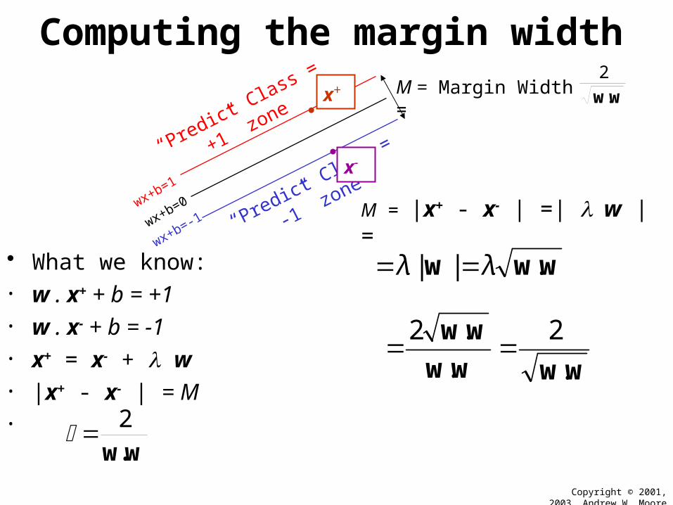
• What we know:• w . x+ + b = +1 • w . x- + b = -1 • x+ = x- + w• |x+ - x- | = M•
“Predict Class = +1” zone
“Predict Class = -1” zone
wx+b=1
wx+b=0
wx+b=-1
M = Margin Width =
M = |x+ - x- | =| w |=
x-
x+
w.w2
wwww
ww
.
2
.
.2
www .|| λλ
ww.
2
Copyright © 2001, 2003, Andrew W. Moore
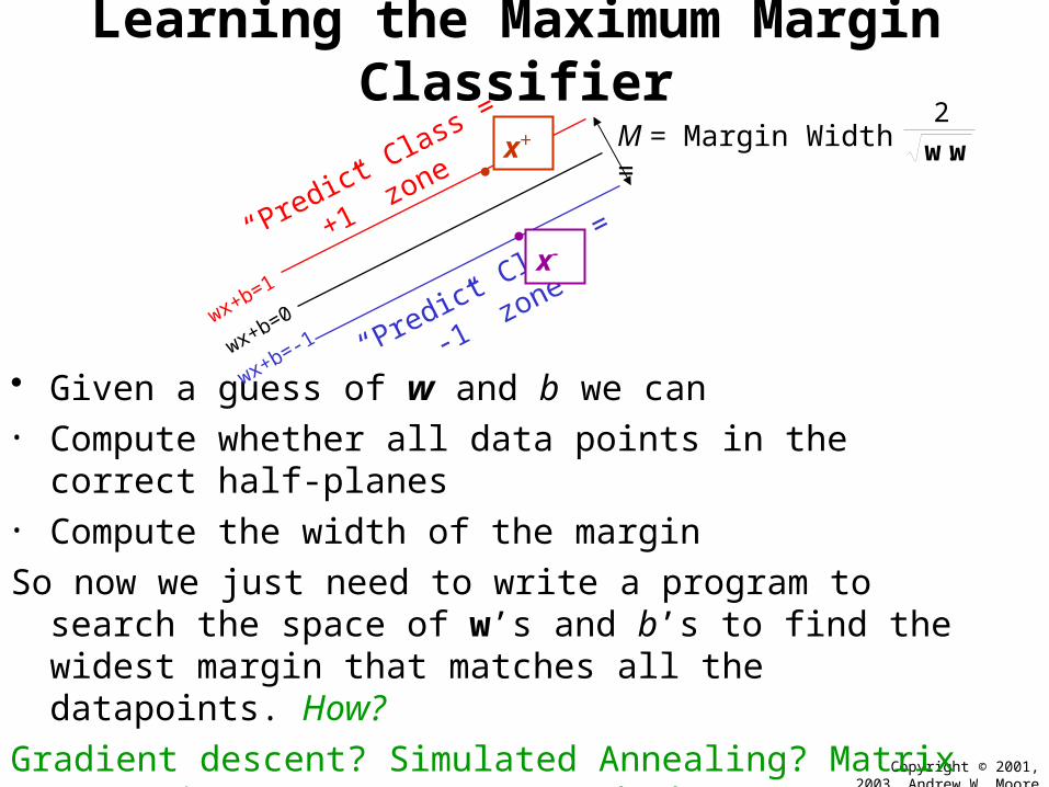
Learning the Maximum Margin Classifier
• Given a guess of w and b we can• Compute whether all data points in the correct half-planes• Compute the width of the margin
So now we just need to write a program to search the space of w’s and b’s to find the widest margin that matches all the datapoints. How?
Gradient descent? Simulated Annealing? Matrix Inversion? EM? Newton’s Method?
“Predict Class = +1” zone
“Predict Class = -1” zone
wx+b=1
wx+b=0
wx+b=-1
M = Margin Width =
x-
x+ ww.
2
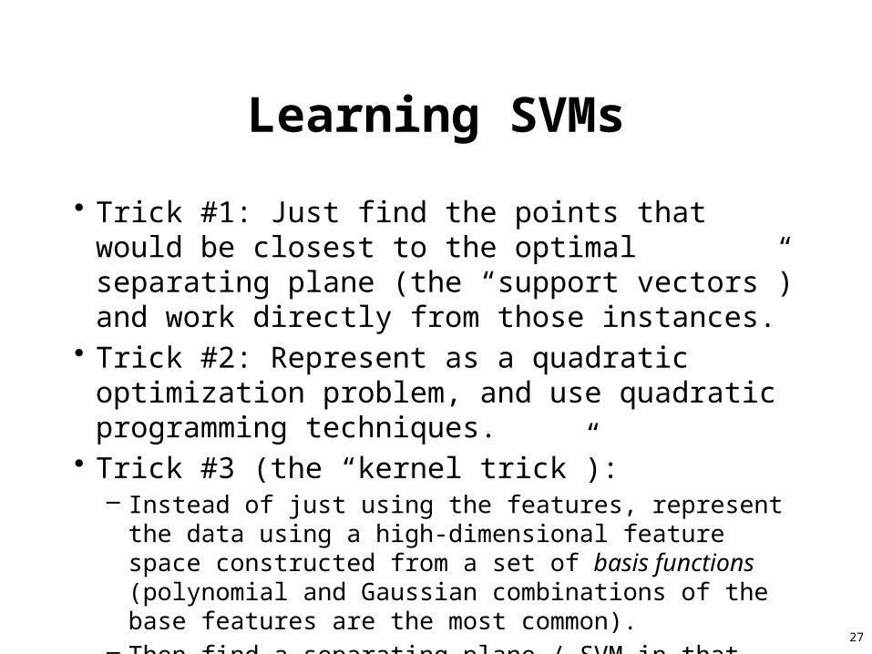
Learning SVMs
• Trick #1: Just find the points that would be closest to the optimal separating plane (the “support vectors”) and work directly from those instances.
• Trick #2: Represent as a quadratic optimization problem, and use quadratic programming techniques.
• Trick #3 (the “kernel trick”): – Instead of just using the features, represent the data using a high-
dimensional feature space constructed from a set of basis functions (polynomial and Gaussian combinations of the base features are the most common).
– Then find a separating plane / SVM in that high-dimensional space– Voila: A nonlinear classifier!
27

Copyright © 2001, 2003, Andrew W. Moore
Common SVM basis functions
zk = ( polynomial terms of xk of degree 1 to q )
zk = ( radial basis functions of xk )
zk = ( sigmoid functions of xk )
KW
||KernelFn)(][ jk
kjk φjcx
xz

Copyright © 2001, 2003, Andrew W. Moore
SVM Performance• Anecdotally they work very very well indeed.• Example: They are currently the best-known classifier on a well-
studied hand-written-character recognition benchmark• Another Example: Andrew knows several reliable people doing
practical real-world work who claim that SVMs have saved them when their other favorite classifiers did poorly.
• There is a lot of excitement and religious fervor about SVMs as of 2001.

Unsupervised Learning:Clustering
30
Unsupervised Learning
• Learn without a “supervisor” who labels instances– Clustering– Scientific discovery– Pattern discovery– Associative learning
• Clustering:– Given a set of instances without labels, partition them such that each
instance is:• similar to other instances in its partition (inter-cluster similarity)• dissimilar from instances in other partitions (intra-cluster dissimilarity)
31
Clustering Techniques
• Partitional clustering– k-means clustering
• Agglomerative clustering– Single-link clustering– Complete-link clustering– Average-link clustering
• Spectral clustering
32

33
Formal Data Clustering
• Data clustering is: – Dividing a set of data objects into groups such that there
is a clear pattern (e.g. similarity to each other) for why objects are in the same cluster
• A clustering algorithm requires:– A data set D– A clustering description C– A clustering objective Obj(C)– An optimization method Opt(D) ~ C
• Obj measures the goodness of the best clustering C that Opt(D) can find

34
What does D look like?
Training Set
6.3,2.5,5.0,1.9,Iris-virginica 6.5,3.0,5.2,2.0,Iris-virginica 6.2,3.4,5.4,2.3,Iris-virginica 5.9,3.0,5.1,1.8,Iris-virginica
5.7,3.0,4.2,1.2,Iris-versicolor 5.7,2.9,4.2,1.3,Iris-versicolor 6.2,2.9,4.3,1.3,Iris-versicolor 5.1,2.5,3.0,1.1,Iris-versicolor
5.1,3.4,1.5,0.2,Iris-setosa 5.0,3.5,1.3,0.3,Iris-setosa 4.5,2.3,1.3,0.3,Iris-setosa 4.4,3.2,1.3,0.2,Iris-setosa
Test Set
5.1,3.5,1.4,0.2,?? 4.9,3.0,1.4,0.2,?? 4.7,3.2,1.3,0.2,?? 4.6,3.1,1.5,0.2,?? 5.0,3.6,1.4,0.2,?? 5.4,3.9,1.7,0.4,?? 4.6,3.4,1.4,0.3,?? 5.0,3.4,1.5,0.2,?? 4.4,2.9,1.4,0.2,?? 4.9,3.1,1.5,0.1,?? 5.4,3.7,1.5,0.2,?? 4.8,3.4,1.6,0.2,??
Supervised learning (KNN, C.45, SVM, etc.)

35
What does D look like?
Training Set
6.3,2.5,5.0,1.9,?? 6.5,3.0,5.2,2.0,?? 6.2,3.4,5.4,2.3,?? 5.9,3.0,5.1,1.8,??
5.7,3.0,4.2,1.2,?? 5.7,2.9,4.2,1.3,?? 6.2,2.9,4.3,1.3,?? 5.1,2.5,3.0,1.1,??
5.1,3.4,1.5,0.2,?? 5.0,3.5,1.3,0.3,?? 4.5,2.3,1.3,0.3,?? 4.4,3.2,1.3,0.2,??
Test Set
5.1,3.5,1.4,0.2,?? 4.9,3.0,1.4,0.2,?? 4.7,3.2,1.3,0.2,?? 4.6,3.1,1.5,0.2,?? 5.0,3.6,1.4,0.2,?? 5.4,3.9,1.7,0.4,?? 4.6,3.4,1.4,0.3,?? 5.0,3.4,1.5,0.2,?? 4.4,2.9,1.4,0.2,?? 4.9,3.1,1.5,0.1,?? 5.4,3.7,1.5,0.2,?? 4.8,3.4,1.6,0.2,??
Un-supervised learning (Clustering!)

36
What does C look like?
• After clustering, the output looks like a ‘labeled’ data set for a supervised learning algorithm: – 6.3,2.5,5.0,1.9,1
6.5,3.0,5.2,2.0,1
6.2,3.4,5.4,2.3,1
5.9,3.0,5.1,1.8,1
5.7,3.0,4.2,1.2,2
5.7,2.9,4.2,1.3,2
6.2,2.9,4.3,1.3,2
5.1,2.5,3.0,1.1,2
5.1,3.4,1.5,0.2,3
5.0,3.5,1.3,0.3,3
4.5,2.3,1.3,0.3,3
4.4,3.2,1.3,0.2,3
11 1 1 2 2 2 23 3 3 3
Clustering Vector

37
Big Questions About Clustering
• How do we even begin clustering?• How do we know we’ve found anything?• How do we know if what we found is even useful?
– How to evaluate the results?
• What do we apply this to?– What’s the truth, versus the hope, of reality?
38
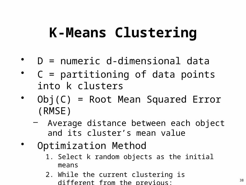
K-Means Clustering
• D = numeric d-dimensional data• C = partitioning of data points into k clusters• Obj(C) = Root Mean Squared Error (RMSE)
– Average distance between each object and its cluster’s mean value
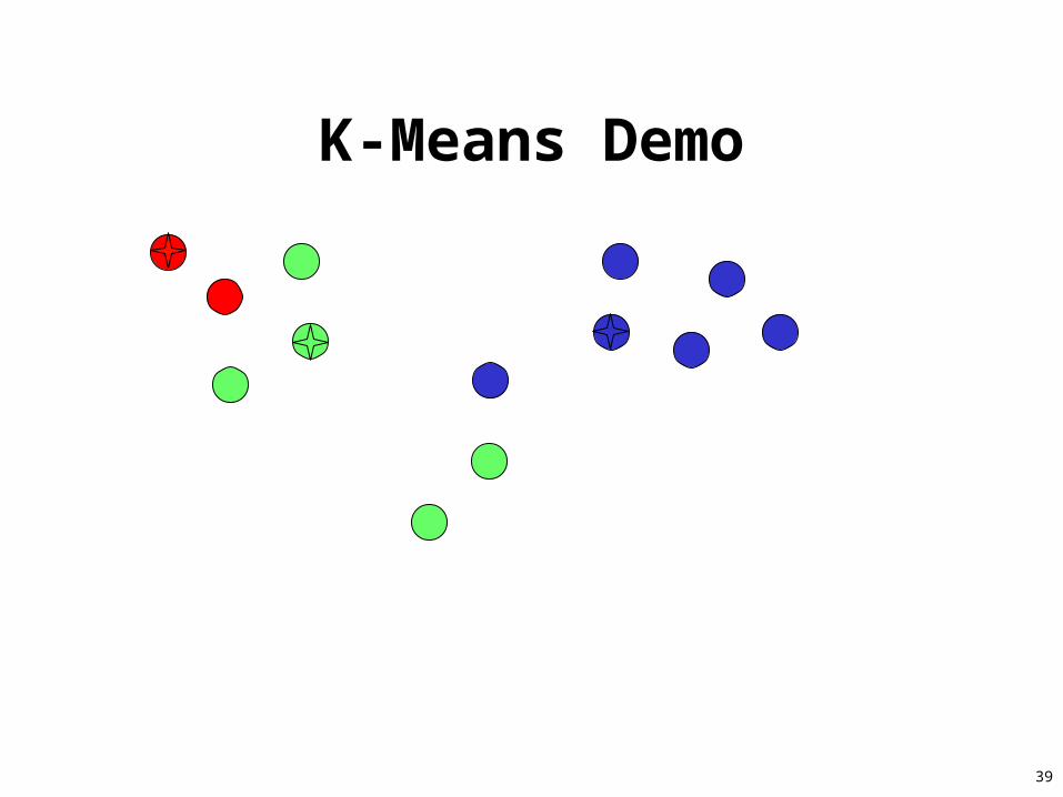
• Optimization Method1. Select k random objects as the initial means
2. While the current clustering is different from the previous:1. Move each object to the cluster with the closest mean
2. Re-compute the cluster means
39
K-Means Demo
40
K-Means Comments
• K-means has some randomness in its initialization, which means: – Two different executions on the same data, same number of clusters
will likely have different results– Two different executions may have very different run-times due to
the convergence test
• In practice, run multiple times and take result with the best RMSE

41
___-Link Clustering
1. Initialize each object in its own cluster2. Compute the cluster distance matrix M by the
selected criterion (below)3. While there is more than k clusters:
1. Join the clusters with the shortest distance 2. Update M by the selected criterion
• Criterion for ___-link clustering– Single-link: use the distance of the closest objects
between two clusters– Complete-link: use the distance of the most distant
objects between the two clusters

42
___-Link Demo
• How can we measure the distance between these clusters?
• What is best for: – Spherical data (above)?– Chain-like data?
Single-Link Distance
Complete-Link Distance
43
___-Link Comments
• The –Link algorithms are not random in any way, which means: – You’ll get the same results whenever you use the same data and
same number of clusters
• Choosing between these algorithms, and K-means (or any other clustering algorithm) requires lots of research, and careful analysis

44
My Research: Relational Data Clustering

45
• The task of organizing objects into logical groups, or clusters, taking into account the relational links between objects
Relational Data Clustering is:

46
Relational Data• Formally:
– A set of object domains– Sets of instances from those domains– Sets of relational tuples, or links between instances
• In Practice:– “Relational data” refers only to data that necessitates the use of links– Information not encoded using a relation is referred to as an attribute
• Spaces:– Attribute space = Ignore relations– Relation space = Ignore attributes
Person(Sally)Person(Fred)Person(J oe)Gender(Sally,F)Gender(Fred,M)Gender(J oe,M)Friends(Sally,Fred)Friends(Fred,J oe)
PeopleName Gender
Sally F
Fred M
Joe M
FriendsSally Fred
Fred Joe
{Sally,F} {Joe,M}
{Fred,M}
47
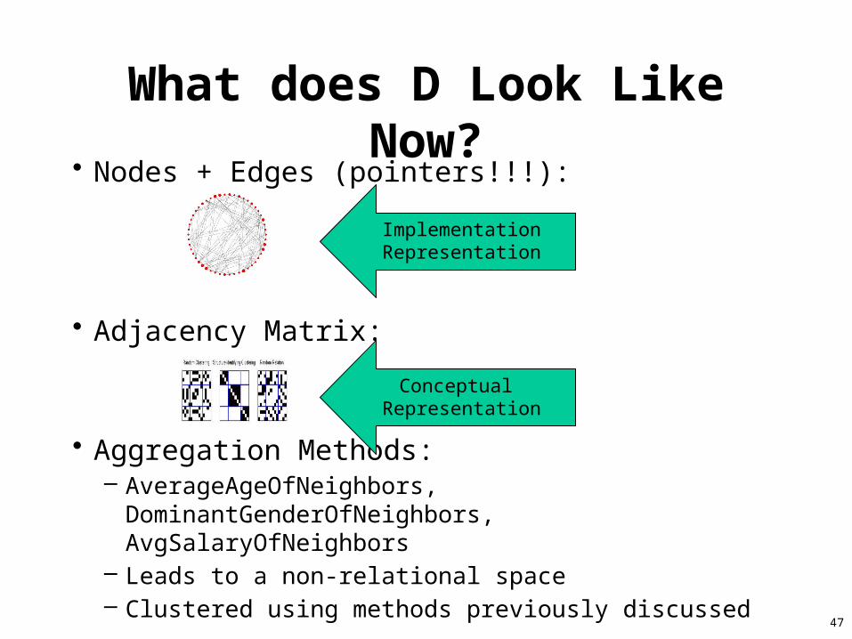
What does D Look Like Now?• Nodes + Edges (pointers!!!):
• Adjacency Matrix:
• Aggregation Methods: – AverageAgeOfNeighbors, DominantGenderOfNeighbors,
AvgSalaryOfNeighbors– Leads to a non-relational space– Clustered using methods previously discussed
Implementation Representation
Conceptual Representation
48
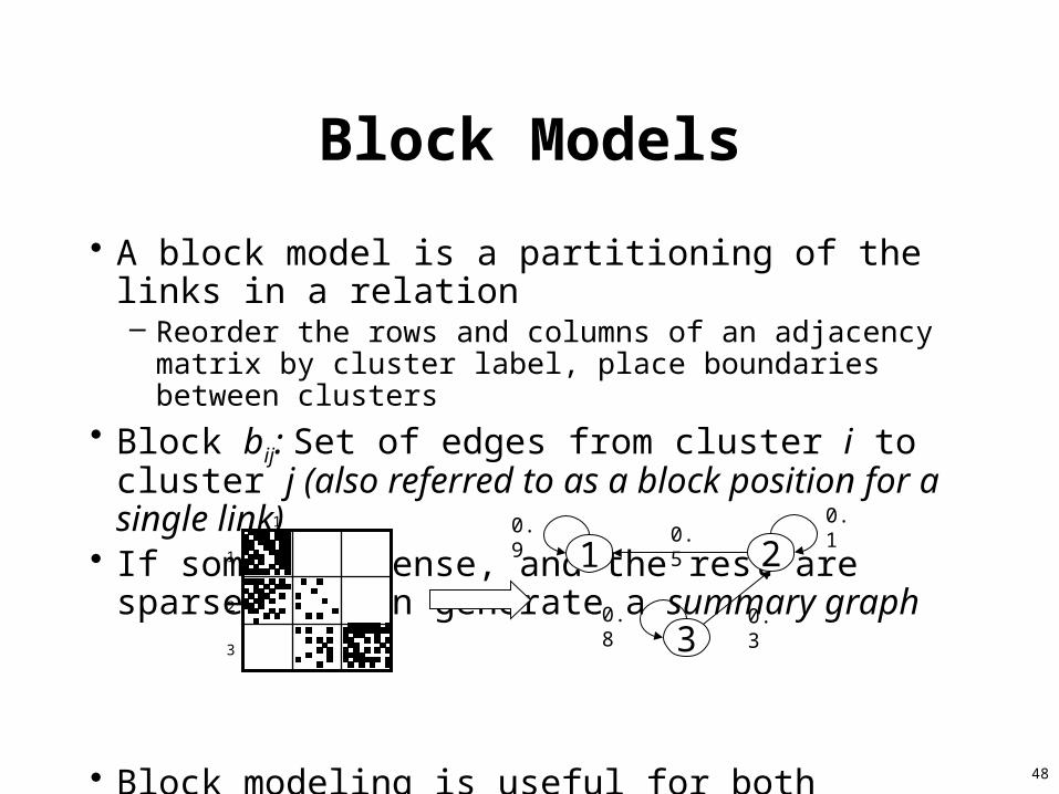
Block Models
• A block model is a partitioning of the links in a relation – Reorder the rows and columns of an adjacency matrix by cluster
label, place boundaries between clusters
• Block bij: Set of edges from cluster i to cluster j (also referred to as a block position for a single link)
• If some are dense, and the rest are sparse, we can generate a summary graph
• Block modeling is useful for both visualization and numerical analysis
1 2 3
1
2
3
1
3
20.9 0.5
0.1
0.30.8

49
Two Relational Clustering Algorithms
Community Detection• Maximizes connectivity within clusters
and minimizes connectivity between clusters
• Intuitive concept that links identify classes
• Equivalent to maximizing density only on the diagonal blocks
• Faster than more general relational clustering approaches
Stochatic Block Modeling• Maximizes the likelihood that two
objects in the same cluster have the same linkage pattern– Linkage may be within, or between
clusters• Subsumes community detection• Equivalent to maximizing density in
any block, rather than just the diagonal• Generalizes relational clustering

50
My Work: Block Modularity
• General block-model-based clustering approach• Models relations only• Motivated by poor scalability of stochastic block
modeling– Would be useful to have a block modeling approach that
scales as well as community detection algorithms• Contributions:
– A clearly defined measure of general relational structure (block modularity)
– An Iterative clustering algorithm that is much faster than prior works

51
Relational Structure
•What is “structure” –High level: non-randomness
–Relational structure: non-random connectivity pattern• A relation is structured if its observed
connectivity pattern is clearly distinguished from that of a random relation
52
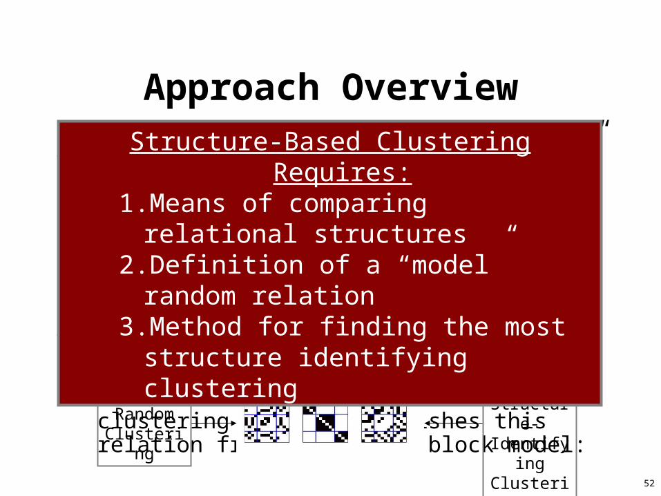
Approach Overview
• Assume that there exists a “model” random relation:
• In contrast, for any non-random relation:– There should exist at least one clustering that
distinguishes this relation from the random block model:
Random Clustering
Structure-Identifying Clustering
Any clustering of this relation will have a similar block model
Structure-Based Clustering Requires:1. Means of comparing relational structures 2. Definition of a “model” random relation3. Method for finding the most structure
identifying clustering

53
Comparing Structure: Block Modularity• Given an input relation, a model random relation*, and a structure-
identifying clustering, we compute block modularity: 1. Find the block model for each relation:
2. Compute the absolute difference of the number of links in each block:
3. Compute the sum of all the cells in the difference matrix: 1584. (Optional) Normalize value by twice the number of links: 0.4389
60 0 0
33 9 18
0 14 46
20 20 20
20 20 20
20 20 20
40 20 20
13 11 2
20 6 26
Input Relation
Model Random Relation
*Required: the model random relation should have the same number of links as the input relation
54
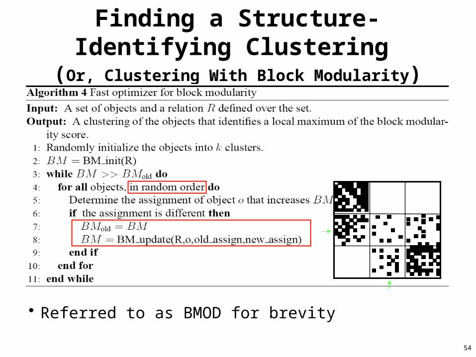
Finding a Structure-Identifying Clustering
(Or, Clustering With Block Modularity)
• Referred to as BMOD for brevity

55
Experimental Evaluation• Work-in-Progress• Past Evaluation: Comparing with small, manageable data
sets to evaluate increase in speed• New Ideas:
– Non-Block-Modeling algorithm is a current popular approach• Is BMOD faster than it? If not, how much slower?
– SCALING UP• Demonstrated speed on “small” data sets
– ~3000 nodes, 4000 edges• How would we do on, say, Facebook?
– 500 M nodes, given avg. 100 friends per node, 5 B edges– Challenges:
• Can’t download Facebook or any data source that is comparable• How to generate a ‘realistic’ artificial data set that has similar features
as FB?– Anyone want to help???
56
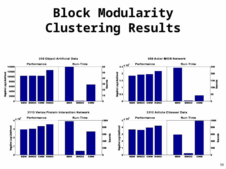
Block Modularity Clustering Results
Methodology57
• Goals: assess speed, accuracy of block modularity vs. leading stochastic method– Degree-Corrected Stochastic Block Model (DCBM) (Karrer &
Newman, 2011)
• Accuracy: Normalized Mutual Information• Data: Generated using DCBM (next slide)
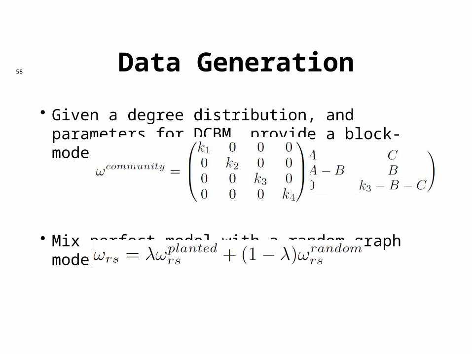
Data Generation58
• Given a degree distribution, and parameters for DCBM, provide a block-model configuration matrix:
• Mix perfect model with a random graph model:

Results59
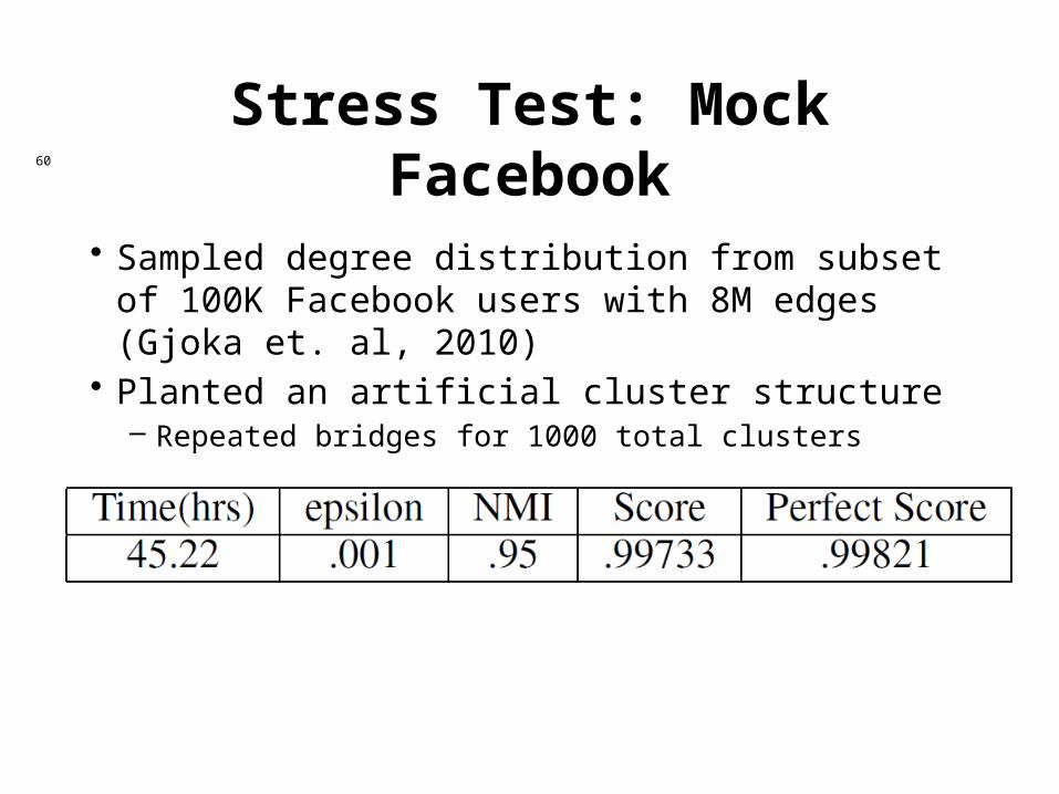
Stress Test: Mock Facebook60
• Sampled degree distribution from subset of 100K Facebook users with 8M edges (Gjoka et. al, 2010)
• Planted an artificial cluster structure– Repeated bridges for 1000 total clusters
Future Work61
• 1000’s of clusters: getting nowhere fast?– Post-analysis and applications– Information Propagation
• Map/Reduce Implementation
62
Conclusion
• Fast and effective when compared to stochastic block modeling
• Iterative, and requires some basic counting mechanisms– Much simpler and less error-prone than implementing a
stochastic algorithm– Fewer mathematical prerequisites makes the algorithm
accessible to more programmers
• A measure of structure, not just an identifier, and its value can be used for other applications