1 CS 552/652 Speech Recognition with Hidden Markov Models Winter 2011 Oregon Health & Science...

1

CS 552/652Speech Recognition with Hidden Markov Models

Winter 2011

Oregon Health & Science UniversityCenter for Spoken Language Understanding

John-Paul Hosom

Lecture 3January 10

Review of Probability & Statistics; Markov Models

2

Review of Probability and Statistics

Random Variables:

• “variable” because different values are possible

• “random” because observed value depends on outcome of some experiment

• discrete random variables:set of possible values is a discrete set

• continuous random variables:set of possible values is an interval of numbers

• usually a capital letter is used to denote a random variable.

3

Probability Density Functions:

• If X is a continuous random variable, then the p.d.f. of X is a function f(x) such that

so that the probability that X has a value between a and b is the area of the density function from a to b.

• Note: f(x) 0 for all xarea under entire graph = 1

• Example 1:


b

adxxfbXaP )()(

f(x)

xa b

4

Probability Density Functions:

• Example 2:


f(x)

xa=0.25 b=0.75

0)( otherwise 10)1(2

3)( 2 xfxxxf

Probability that x is between 0.25 and 0.75 is

547.0)3

(2

3)1(

2

3)75.025.0(

75.0

25.0

375.0

25.0

2

x

x

xxdxxxP

from Devore, p. 134

5

Cumulative Distribution Functions:

• cumulative distribution function (c.d.f.) F(x) for c.r.v. X is:

• example:


f(x)

xb=0.75


3)( 2 xfxxxf

C.D.F. of f(x) is

)3

(2

3)

3(

2

3)1(

2

3)(

3

0

3

0

2 xx

yydyyxF

xy

y

x

x

dyyfxXPxF )()()(

6

• Expected Values:

• expected (mean) value of c.r.v. X with p.d.f. f(x) is:

• example 1 (discrete):

• example 2 (continuous):


dxxfxXEX )()(

E(X) = 2·0.05+3·0.10+ … +9·0.05 = 5.35

0.05

0.250.20

0.150.10

0.15

0.05 0.05

1.0 2.0 3.0 4.0 5.0 6.0 7.0 8.0 9.0

8

3)

42(

2

3)(

2

3)1(

2

3)(

1

0

421

0

31

0

2

x

x

xxdxxxdxxxXE


3)( 2 xfxxxf

Or, take 3 numbers: 45, 20, and 12 from some populationof numbers. The mean is (45+20+12+31)/4=27. Theexpected value is ¼×45 + ¼×20 + ¼×12 + ¼×31 = 27, since the probability of any of these 4 values is equally likely at 25%. So the mean and the expected value arethe same.

7


The Normal (Gaussian) Distribution:

• the p.d.f. of a Normal distribution is

xxf x 22 2/)(e2

1),;(

where μ is the mean and σ is the standard deviation

μ

σ

σ2 is called the variance.

8


The Normal (Gaussian) Distribution:

• Any arbitrary p.d.f. can be constructed by summing N weighted Gaussians (mixtures of Gaussians)

w1 w2 w3 w4 w5 w6

• This is what is meant by a “Gaussian Mixture Model” (GMM)

9


Conditional Probability:

• event space

• the conditional probability of event A given that event B has occurred:

)(

)()|(

BP

BAPBAP

• the multiplication rule:)()|()( BPBAPBAP

A

B

10

Conditional Probability: Example (from Devore, p.52)

• 3 equally-popular airlines (1,2,3) fly from LA to NYC.Probability of 1 being delayed: 40%Probability of 2 being delayed: 50%Probability of 3 being delayed: 70%

• probability of selecting an airline=A, probability of delay=B


P(A 1 ) = 1/3

P(B|A3) = 7/10P(A3B) = 1/3 × 7/10 = 7/30

P(B’|A3) = 3/10

Late = B

Not Late = B’

A3 = Airline 3

P(B|A1) = 4/10 P(A1B) = 1/3 × 4/10 = 4/30

P(B’|A1) = 6/10

Late = B

Not Late = B’A 1

= Airline 1

P(A3 ) = 1/3

P(B|A2) = 5/10 P(A2B) = 1/3 × 5/10 = 5/30P(B’|A

2) = 5/10Late = B

Not Late = B’

A2 = Airline 2P(A2 ) = 1/3

11

Conditional Probability: Example (from Devore, p.52)

• What is probability of choosing airline 1 and being delayed on that airline?

• What is probability of being delayed?

• Given that the flight was delayed, what is probability that the airline is 1?


133.030

4

10

4

3

1)|()()( 111 ABPAPBAP

30

16

30

7

30

5

30

4321 )()()()( BAPBAPBAPBP

4

1

3016

304

)(

)()|( 1

1

BP

BAPBAP

12


Law of Total Probability:

• for independent events A1, A2, … An and any other event B:

Bayes’ Rule:

• for independent events A1, A2, … An and any other event B, with P(Ai) > 0 and P(B) > 0:

n

iii APABPBP

1

)()|()(

)(

)()|(

BP

BAPBAP k

k

)(

)()|(

)()|(

)()|(

1

BP

APABP

APABP

APABP kkn

iii

kk

13


Independence:

• events A and B are independent iff

• from multiplication rule or from Bayes’ rule,

• from multiplication rule and definition of independence, events A and B are independent iff

)()|( APBAP

)(

)()|(

)(

)()|(

AP

BPBAP

AP

BAPABP

)()()( BPAPBAP

14

A Markov Model (Markov Chain) is:

• similar to a finite-state automata, with probabilities of transitioning from one state to another:

What is a Markov Model?

S1 S5S2 S3 S4

0.5

0.5 0.3

0.7

0.1

0.9 0.8

0.2

• transition from state to state at discrete time intervals

• can only be in 1 state at any given time

1.0

15

Elements of a Markov Model (Chain):

• clockt = {1, 2, 3, … T}

• N statesQ = {1, 2, 3, … N}the single state j at time t is referred to as qt

• N eventsE = {e1, e2, e3, …, eN}

• initial probabilitiesπj = P[q1 = j] 1 j N

• transition probabilitiesaij = P[qt = j | qt-1 = i] 1 i, j N


16

Elements of a Markov Model (chain):

• the (potentially) occupied state at time t is called qt

• a state can referred to by its index, e.g. qt = j

• 1 event corresponds to 1 state:

At each time t, the occupied state outputs (“emits”)its corresponding event.

• Markov model is generator of events.

• each event is discrete, has single output.

• in typical finite-state machine, actions occur at transitions, but in most Markov Models, actions occur at each state.


17

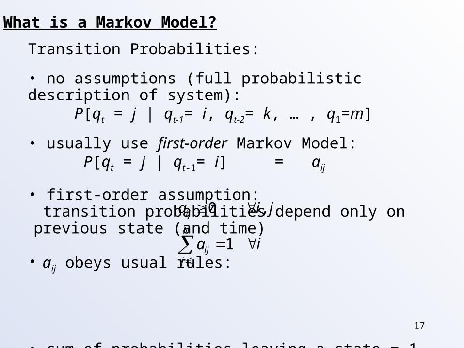
Transition Probabilities: • no assumptions (full probabilistic description of system):

P[qt = j | qt-1= i, qt-2= k, … , q1=m]

• usually use first-order Markov Model: P[qt = j | qt-1= i] = aij

• first-order assumption: transition probabilities depend only on previous state (and time)

• aij obeys usual rules:

• sum of probabilities leaving a state = 1 (must leave a state)


N

jij

ij

ia

jia

1

1

,0

18

S1 S2 S3

0.5

0.5 0.3

0.7

Transition Probabilities: • example:


a11 = 0.0 a12 = 0.5 a13 = 0.5 a1Exit=0.0 =1.0a21 = 0.0 a22 = 0.7 a23 = 0.3 a2Exit=0.0 =1.0a31 = 0.0 a32 = 0.0 a33 = 0.0 a3Exit=1.0 =1.0

1.0

19

Transition Probabilities: • probability distribution function:


S1 S2 S30.6

0.4

p(being in state S2 exactly 1 time) = 0.6 = 0.600p(being in state S2 exactly 2 times) = 0.4 ·0.6 = 0.240p(being in state S2 exactly 3 times) = 0.4 ·0.4 ·0.6 = 0.096p(being in state S2 exactly 4 times) = 0.4 ·0.4 ·0.4 ·0.6 = 0.038

= exponential decay (characteristic of Markov Models)

20

Transition Probabilities:


S1 S2 S30.1

0.9p(being in state S2 exactly 1 time) = 0.1 = 0.100p(being in state S2 exactly 2 times) = 0.9 ·0.1 = 0.090p(being in state S2 exactly 3 times) = 0.9 ·0.9 ·0.1 = 0.081p(being in state S2 exactly 5 times) = 0.9 ·0.9 · ... ·0.1 = 0.059

a22=0.9

a22=0.5

(note:in graph, nomultiplication by a23)

a22=0.7

prob

. of

bein

g in

sta

te

length of time in same state

21

Transition Probabilities: • can construct second-order Markov Model:

P[qt = j | qt-1= i, qt-2= k]


S1

S3

S2

qt-2=S2: 0.15qt-2=S3: 0.25

qt-2=S1:0.3

qt-2=S1:0.25

qt-2=S1:0.2

qt-2=S2:0.1qt-2=S3:0.2

qt-2=S2:0.2 qt-2=S2:0.3

qt-2=S3:0.35

qt-2=S1:0.10qt-2=S3:0.30

22

Initial Probabilities: • probabilities of starting in each state at time 1

• denoted by πj

• πj = P[q1 = j] 1 j N

•


11

N

jj

23

• Example 1: Single Fair Coin


S1 S2

0.5

0.5

0.5 0.5

S1 corresponds to e1 = Heads a11 = 0.5 a12 = 0.5S2 corresponds to e2 = Tails a21 = 0.5 a22 = 0.5

• Generate events:H T H H T H T T T H H

corresponds to state sequenceS1 S2 S1 S1 S2 S1 S2 S2 S2 S1 S1

24

• Example 2: Single Biased Coin (outcome depends on previous result)


S1 S2

0.3

0.4

0.7 0.6

S1 corresponds to e1 = Heads a11 = 0.7 a12 = 0.3S2 corresponds to e2 = Tails a21 = 0.4 a22 = 0.6

• Generate events:H H H T T T H H H T T H

corresponds to state sequenceS1 S1 S1 S2 S2 S2 S1 S1 S1 S2 S2 S1

25

• Example 3: Portland Winter Weather


S1S2

0.25

0.4

0.7 0.5

S3

0.20.05

0.70.1

0.1

26

• Example 3: Portland Winter Weather (con’t)

• S1 = event1 = rain S2 = event2 = clouds A = {aij} = S3 = event3 = sun

• what is probability of {rain, rain, rain, clouds, sun, clouds, rain}?Obs. = {r, r, r, c, s, c, r}S = {S1, S1, S1, S2, S3, S2, S1}time = {1, 2, 3, 4, 5, 6, 7} (days)

= P[S1] P[S1|S1] P[S1|S1] P[S2|S1] P[S3|S2] P[S2|S3] P[S1|S2]

= 0.5 · 0.7 · 0.7 · 0.25 · 0.1 · 0.7 · 0.4

= 0.001715


10.70.20.

10.50.40.

05.25.70. π1 = 0.5π2 = 0.4π3 = 0.1

27

• Example 3: Portland Winter Weather (con’t)

• S1 = event1 = rain S2 = event2 = clouds A = {aij} = S3 = event3 = sunny

• what is probability of {sun, sun, sun, rain, clouds, sun, sun}?Obs. = {s, s, s, r, c, s, s}S = {S3, S3, S3, S1, S2, S3, S3}time = {1, 2, 3, 4, 5, 6, 7} (days)

= P[S3] P[S3|S3] P[S3|S3] P[S1|S3] P[S2|S1] P[S3|S2] P[S3|S3]

= 0.1 · 0.1 · 0.1 · 0.2 · 0.25 · 0.1 · 0.1

= 5.0x10-7


10.70.20.

10.50.40.

05.25.70. π1 = 0.5π2 = 0.4π3 = 0.1

28

• Example 4: Marbles in Jars (lazy person)


Jar 1 Jar 2 Jar 3

S1 S2

0.3

0.2

0.6 0.6

S3

0.10.1

0.30.2

0.6

(assume unlimited number of marbles)

29

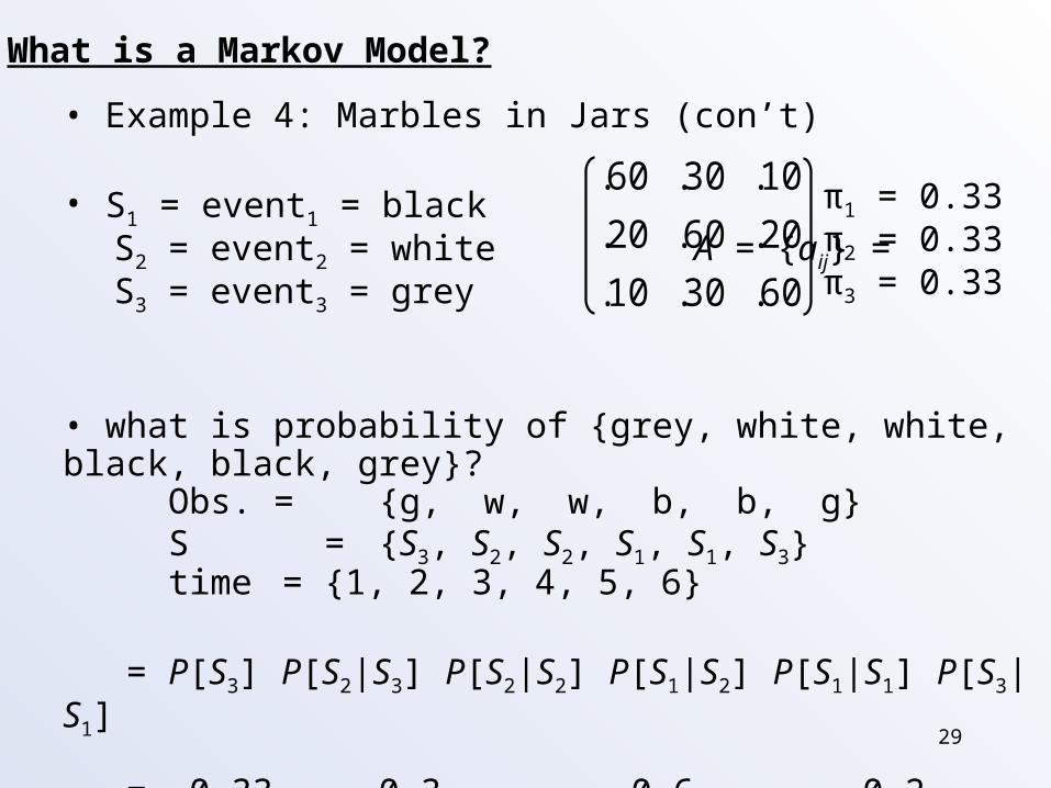
• Example 4: Marbles in Jars (con’t)

• S1 = event1 = black S2 = event2 = white A = {aij} = S3 = event3 = grey

• what is probability of {grey, white, white, black, black, grey}?Obs. = {g, w, w, b, b, g}S = {S3, S2, S2, S1, S1, S3}time = {1, 2, 3, 4, 5, 6}

= P[S3] P[S2|S3] P[S2|S2] P[S1|S2] P[S1|S1] P[S3|S1]

= 0.33 · 0.3 · 0.6 · 0.2 · 0.6 · 0.1 = 0.0007128


60.30.10.

20.60.20.

10.30.60. π1 = 0.33π2 = 0.33π3 = 0.33

30

• Example 4A: Marbles in Jars


Jar 1 Jar 2 Jar 3

S1 S2

0.3

0.2

0.6 0.6

S3

0.10.1

0.30.2

0.6

S1 S2

0.33

0.33

0.33 0.33

S3

0.330.33

0.330.33

0.33• Same data, two different models...

“lazy” “random”

31

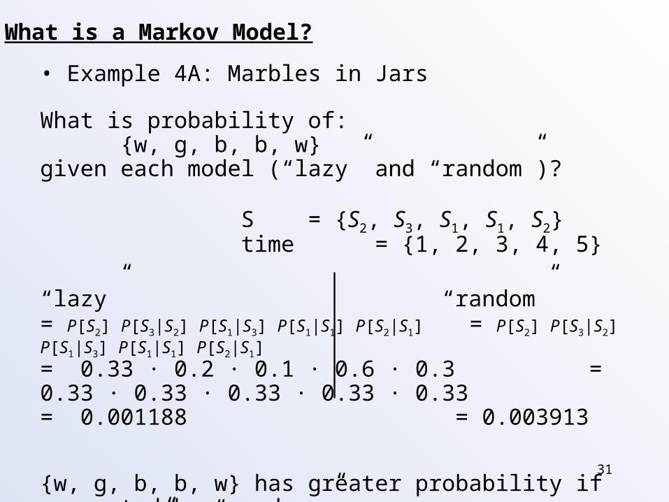
• Example 4A: Marbles in Jars

What is probability of: {w, g, b, b, w}

given each model (“lazy” and “random”)?

S = {S2, S3, S1, S1, S2}time = {1, 2, 3, 4, 5}

“lazy” “random”= P[S2] P[S3|S2] P[S1|S3] P[S1|S1] P[S2|S1] = P[S2] P[S3|S2] P[S1|S3] P[S1|S1] P[S2|S1]

= 0.33 · 0.2 · 0.1 · 0.6 · 0.3 = 0.33 · 0.33 · 0.33 · 0.33 · 0.33= 0.001188 = 0.003913

{w, g, b, b, w} has greater probability if generated by “random.”“random” model more likely to generate {w, g, b, b, w}.


32

Notes:

• Independence is assumed between events that are separated by more than one time frame, when computing probability of sequence of events (for first-order model).

• Given list of observations, we can determine exact state sequence that generated those observations. state sequence not hidden.

• Each state associated with only one event (output).

• Computing probability given a set of observations and a model is straightforward.

• Given multiple Markov Models and an observation sequence, it’s easy to determine the M.M. most likely to have generated the data.


1 CS 552/652 Speech Recognition with Hidden Markov Models Winter 2011 Oregon Health & Science...

Documents

Transcript of 1 CS 552/652 Speech Recognition with Hidden Markov Models Winter 2011 Oregon Health & Science...