1 Consensus Computation in Unreliable Networks: A System ...

1

Consensus Computation in Unreliable Networks:

A System Theoretic Approach

Fabio Pasqualetti Antonio Bicchi Francesco Bullo

Abstract

This work considers the problem of reaching consensus in an unreliable linear consensus network. A solution tothis problem is relevant for several tasks in multi-agent systems including motion coordination, clock synchronization,and cooperative estimation. By modeling the unreliable nodes as unknown and unmeasurable inputs affecting thenetwork, we recast the problem into an unknown-input system theoretic framework. Only relying on their directmeasurements, the agents detect and identify the misbehaving agents using fault detection and isolation techniques. Weconsider both the case that misbehaviors are simply caused by faults, or that they are the product of a definite, malignant“Byzantine” strategy. We express the solvability conditions of the two cases in a system theoretic framework, and froma graph theoretic perspective. We show that generically any node can correctly detect and identify the misbehavingagents, provided that the connectivity of the network is sufficiently high. Precisely, for a linear consensus networkto be generically resilient to k concurrent faults, the connectivity of the communication graph needs to be 2k + 1, ifByzantine agents are allowed, and k + 1, if non-colluding agents are considered. We finally provide algorithms fordetecting and isolating misbehaving agents. The first procedure applies standard fault detection techniques, and affordscomplete intrusion detection if global knowledge of the graph is available to each agent, at a high computational cost.The second method is designed to exploit the presence in a network of weakly interconnected subparts, and providescomputationally efficient detection of misbehaving agents whose behavior deviates more than a threshold, which isquantified in terms of the interconnection structure.

I. INTRODUCTION

Distributed systems and networks have received much attention in the last years because of their flexibility and

computational performance. One of the most frequent tasks to be accomplished by autonomous agents is to agree

upon some parameters. Agreement variables represent quantities of interest such as the work load in a network of

parallel computers, the clock speed for wireless sensor networks, the velocity, the rendezvous point, or the formation

pattern for a team of autonomous vehicles; e.g., see [1], [2], [3].

Several algorithms achieving consensus have been proposed and studied in the computer science community [4].

In this work, we consider linear consensus iterations, where, at each time instant, each node updates its state as

This material is based upon work supported in part by the ARO Institute for Collaborative Biotechnology award DAAD19-03-D-0004, bythe AFOSR MURI award FA9550-07-1-0528, by the Contract IST 224428 (2008) (STREP) “CHAT - Control of Heterogeneous AutomationSystems: Technologies for scalability, reconfigurability and security,” and by the CONET, the Cooperating Objects Network of Excellence,funded by the European Commission under FP7 with contract number FP7-2007-2-224053. The authors thank Dr. Natasha Neogi for insightfulconversations, and the reviewers for their thoughtful and constructive remarks.

Fabio Pasqualetti is with the Center for Control, Dynamical Systems and Computation, University of California, Santa Barbara,[email protected] .

Antonio Bicchi is with the Centro I. R. “E. Piaggio”, Universita di Pisa, [email protected] .Francesco Bullo is with the Center for Control, Dynamical Systems and Computation, University of California, Santa Barbara,

[email protected] .

February 15, 2011 DRAFT

2

a weighted combination of its own value and those received from its neighbors [5], [6]. The choice of algorithm

weights is a parameter that influences the convergence speed toward the steady state value [7].

Because of the lack of a centralized entity that monitors the activity of the nodes of the network, distributed

systems are prone to attacks and components failure, and it is of increasing importance to guarantee trustworthy

computation even in the presence of misbehaving parts [8]. Misbehaving agents can interfere with the nominal

functions of the network in different ways. In this paper, we consider two extreme cases: that the deviations from

their nominal behavior are due to genuine, random faults in the agents; or that agents can instead craft messages

with the purpose of disrupting the network functions. In the first scenario, faulty agents are unaware of the structure

and state of the network and ignore the presence of other faults. In the second scenario, the worst-case assumption

is made that misbehaving agents have knowledge of the structure and state of the network, and may collude with

others to produce the biggest damage. We refer to the first case as non-colluding, or faulty; to the second case as

malicious, or Byzantine.

Reaching unanimity in an unreliable system is an important problem, well studied by computer scientists interested

in distributed computing. A first characterization of the resilience of distributed systems to malicious attacks appears

in [9], where the authors consider the task of agreeing upon a binary message sent by a “Byzantine general,” when

the communication graph is complete. In [10] the resilience of a partially connected1 network seeking consensus

is analyzed, and it is shown that the well-behaving agents of a network can always agree upon a parameter if and

only if the number of malicious agents

(i) is less than 12 of the network connectivity, and

(ii) is less than 13 of the number of processors.

This result has to be regarded as a fundamental limitation of the ability of a distributed consensus system to sustain

arbitrary malfunctioning: the presence of misbehaving Byzantine processors can be tolerated only if their number

satisfies the above threshold, independently of whatever consensus protocol is adopted.

In this work, we consider linear consensus algorithms in which every agent, including the misbehaving ones, are

assumed to send the same information to all their neighbors. This assumption appears to be realistic for most control

scenarios. In a sensing network for instance, the data used in the consensus protocol consist of the measurements

taken directly by the agents, and it is assumed that the measurements regarding the same quantity coincide. Also,

in a broadcast network, the information is transmitted using broadcast messages, so that the content of a message

is the same for all the receiving nodes. The problem of characterizing the resilience properties of linear consensus

strategies has been partially addressed in recent works [11], [12], [13], where, for the malicious case, it is shown

that, despite the limited abilities of the misbehaving agents, the resilience to external attacks is still limited by

the connectivity of the network. In [11] the problem of detecting and identifying misbehaving agents in a linear

consensus network is first introduced, and a solution is proposed for the single faulty agent case. In [12], [13],

the authors provide one policy that k malicious agents can follow to prevent some of the nodes of a 2k-connected

network from computing the desired function of the initial state, or, equivalently, from reaching an agreement. On

the contrary, if the connectivity is 2k + 1 or more, then the authors show that generically the set of misbehaving

nodes is identified independent of its behavior, so that the desired consensus is eventually reached.

1The connectivity of a graph is the maximum number of disjoint paths between any two vertices of the graph. A graph is complete if it hasconnectivity n− 1, where n is the number of vertices in the graph.


3

The main differences between this paper and the references [12], [13] are as follows. First, the method proposed

in [12], [13] takes inspiration from parity space methods for fault detection, while, following our early work [11],

we adopt here unknown-input observers techniques (cf. [14]). Second, we focus on consensus networks, and we

derive specific results for this important case that cannot be assessed for general linear iterations. Third, we consider

two different types of misbehaving agents, namely malicious and faulty agents, and we provide network resilience

bounds for both cases. Fourth, we exhaustively characterize the complete set of policies that make a set of k agents

undetectable and/or unidentifiable, as opposed to [12] where only a particular disrupting strategy is defined. Fifth,

we study system theoretic properties of consensus systems (e.g., detectability, stabilizability, left-invertibility), and

we quantify the effect of some misbehaving inputs on the network performance. Finally, we address the problem

of detection complexity and we propose a computationally efficient detection method, as opposed to combinatorial

procedures. Our approach also differs from the existing computer science literature, e.g., our analysis leads to

the development of algorithms that can be easily extended to work on both discrete and continuous time linear

consensus networks, and also with partial knowledge of the network topology.

The main contributions of this work are as follows. By recasting the problem of linear consensus computation in

an unreliable system into a system theoretic framework, we provide alternative and constructive system-theoretic

proofs of existing bounds on the number of identifiable misbehaving agents in a linear network, i.e., k Byzantine

agents can be detected and identified if the network is (2k + 1)-connected, and they cannot be identified if the

network is (2k)-connected or less. Moreover, by showing some connections between linear consensus networks

and linear dynamical systems, we exhaustively describe the strategies that misbehaving nodes can follow to disrupt

a linear network that is not sufficiently connected. We prove that the inputs that allow the misbehaving agents to

remain undetected or unidentified coincide with the inputs-zero of a linear system associated with the consensus

network, and they can be ignored if only genuinely faulty agents are considered. For the latter case, we provide

a novel and comprehensive analysis on the detection and identification of non-colluding agents. We show that k

faulty agents can be identified if the network is (k + 1)-connected, and cannot if the network is k-connected or

less. For both the cases of Byzantine and non-colluding agents, we prove that the proposed bounds are generic with

respect to the network communication weights, i.e., given an (unweighted) consensus graph, the bounds hold for

almost all (consensus) choices of the communication weights. In other words, if we are given a (k + 1)-connected

consensus network for which k faulty agents cannot be identified, then a random and arbitrary small change of

the communication weights (within the space of consensus weights) make the misbehaving agents identifiable with

probability one. In the last part of the paper, we discuss the problem of detecting and identifying misbehaving

agents when either the partial knowledge of the network or hardware limitations make it impossible to implement

an exact identification procedure. We introduce a notion of network decentralization, in terms of relatively weakly

connected subnetworks, and derive a sufficient condition on the consensus matrix that allows to identify a certain

class of misbehaving agents under limited information on the network structure, and that ultimately leads to a

prompt recovery of the network functionalities.

The rest of the paper is organized as follows. Section II briefly recalls some basic facts on the geometric approach

to the study of linear systems, and on the fault detection and isolation problem. In Section III we model linear

consensus networks with misbehaving agents. Section IV presents the conditions under which the misbehaving

agents are detectable and identifiable. In Section V we characterize the effect of an unidentifiable attack on the

network consensus state. In Section VI we show that the resilience of linear consensus networks to failures and


4

external attacks is a generic property with respect to the consensus weights. In Section VII we present our algorithmic

procedures. Precisely we derive an exact identification algorithm, and an approximate and low-complexity procedure.

Finally, Sections VIII and IX contain respectively our numerical studies and our conclusion.

II. NOTATION AND PRELIMINARY CONCEPTS

We adopt the same notation as in [15]. Let n, m, p ∈ N, let A ∈ Rn×n, B ∈ Rn×m, and C ∈ Rp×n. Throughout

the paper, let the triple (A,B, C) denote the linear discrete time system

x(t + 1) = Ax(t) + Bu(t),

y(t) = Cx(t),(1)

and let the subspaces B ⊆ Rn×n and C ⊆ Rn×n denote respectively the image space Im(B) and the null space

Ker(C). A subspace V ⊆ Rn×n is a (A,B)-controlled invariant if AV ⊆ V + B, while a subspace S ⊆ Rn×n is a

(A, C)-conditioned invariant if A(S∩C) ⊆ S. The set of all controlled invariants contained in C admits a supremum,

which we denote with V∗, and which corresponds to the locus of all possible state trajectories of (1) invisible at the

output. On the other hand, the set of the conditioned invariants containing B admits an infimum, which we denote

with S∗. Several problems, including disturbance decoupling, non interacting control, fault detection and isolation,

and state estimation in the presence of unknown inputs have been addressed and solved in a geometric framework

[15], [16].

In the classical Fault Detection and Isolation (FDI) setup, the presence of sensor failures and actuator malfunctions

is modeled by adding some unknown and unmeasurable functions ui(t) to the nominal system. The FDI problem

is to design, for each failure i, a filter of the form

wi(t + 1) = Fiwi(t) + Eiy(t),

ri(t) = Miw(t) + Hiy(t),(2)

also known as residual generator, that takes the observables y(t) and generates a residual vector ri(t) that allows to

uniquely identify if ui(t) becomes nonzero, i.e., if the failure i occurred in the system. Let B1, . . . , Bm be the input

matrices of the failure functions u1, . . . , um. As a result of [15], [17], the i-th failure can be correctly identified

if and only if Bi ∩ (V∗K\{i} + S∗K\{i}) = ∅, where V∗K\{i} and S∗K\{i} are the maximal controlled and minimal

conditioned invariant subspaces associated with the triple (A, [B1 · · ·Bi−1 Bi+1 · · ·Bm], C). It can be shown that,

under the above solvability condition, the filter (2) can be designed as a dead beat device to have finite convergence

time [17]: this property will be used in Section VII for the characterization of our intrusion detection algorithm.

We remark that, although the FDI problem does not coincide with the problem we are going to face, we will be

using some standard FDI techniques to design our identification algorithms, and we refer the reader to [14] for a

comprehensive treatment of the subject.

III. LINEAR CONSENSUS IN THE PRESENCE OF MISBEHAVING AGENTS

Let G denote a directed graph with vertex set V = {1, . . . , n} and edge set E ⊂ V × V , and recall that the

connectivity of G is the maximum number of disjoint paths between any two vertices of the graph, or, equivalently,

the minimum number of vertices in a vertex cutset [18]. The neighbor set of a node i ∈ V , i.e., all the nodes j ∈ V

such that the pair (j, i) ∈ E, is denoted with Ni. We let each vertex j ∈ V denote an autonomous agent, and we


5

associate a real number xj with each agent j. Let the vector x ∈ Rn contain the values xj . A linear iteration over

G is an update rule for x and is described by the linear discrete time system

x(t + 1) = Ax(t), (3)

where the (i, j)-th entry of A is nonzero only if (j, i) ∈ E. If the matrix A is row stochastic and primitive, then,

independent of the initial values of the nodes, the network asymptotically converges to a configuration in which

the state of the agents coincides. In the latter case, the matrix A is referred to as a consensus matrix, and the

system (3) is called consensus system. The graph G is referred to as the communication graph associated with the

consensus system (3) or, equivalently, with the consensus matrix A. A detailed treatment of the applications, and

the convergence aspects of the consensus algorithm is in [1], [2], [3], and in the references therein.

We allow for some agents to update their state differently than specified by the matrix A by adding an exogenous

input to the consensus system. Let ui(t), i ∈ V , be the input associated with the i-th agent, and let u(t) be the

vector of the functions ui(t), then the consensus system becomes x(t + 1) = Ax(t) + u(t).

Definition 1 (Misbehaving agent) An agent j is misbehaving if there exists a time t ∈ N such that uj(t) 6= 0.

In Section IV we will give a precise definition of the distinction, made already in the Introduction, between faulty

and malicious agents, on the basis of their inputs.

Let K = {i1, i2, . . . } ⊆ V denote a set of misbehaving agents, and let BK = [ei1 ei2 · · · ], where ei is the i-th

vector of the canonical basis. The consensus system with misbehaving agents K assumes the form

x(t + 1) = Ax(t) + BKuK(t). (4)

As it is shown in [11], algorithms of the form (3) have no resilience to malfunctions, and the presence of

a misbehaving agent may prevent the entire network from reaching consensus. As an example, let c ∈ R, and

let ui(t) = −Aix(t) + c, where Ai denotes the i-th row of A. After reordering the variables in a way that the

well-behaving nodes come first, the consensus system can be rewritten as

x(t + 1) =

[Q R

0 1

]x(t), (5)

where the matrix Q corresponds to the interaction among the nodes V \{i}, while R denotes the connection between

the sets V \ {i} and {i}. Recall that a matrix is said to be Schur stable if all its eigenvalues lie in the open unit

disk.

Lemma III.1 (Quasi-stochastic submatrices) Let A be an n× n consensus matrix, and let J be a proper subset

of {1, . . . , n}. The submatrix with entries Ai,k, i, k ∈ J , is Schur stable.

Proof: Reorder the nodes such that the indexes in J come first in the matrix A. Let AJ be the leading

principal submatrix of dimension |J |. Let AJ =[

AJ 00 0

], where the zeros are such that AJ is n × n, and note

that ρ(AJ) = ρ(AJ), where ρ(AJ) denotes the spectral radius of the matrix AJ [19]. Since A is a consensus

matrix, it has only one eigenvalue of unitary modulus, and ρ(A) = 1. Moreover, A ≥ |AJ |, and A 6= |AJ |, where

|AJ | is such that its (i, j)-th entry equals the absolute value of the (i, j)-th entry of AJ , ∀i, j. It is known that

ρ(AJ) ≤ ρ(A) = 1, and that if equality holds, then there exists a diagonal matrix D with nonzero diagonal entries,


6

such that A = DAJD−1 [20]. Because A is irreducible, there exists no diagonal matrix D with nonzero diagonal

entries such that A = DAJD−1. We conclude that ρ(AJ) < ρ(A) = 1.

Because of Lemma III.1, the matrix Q in (5) is Schur stable, so that the steady state value of the well-behaving

agents in (5) depends upon the action of the misbehaving node, and it corresponds to (I −Q)−1Rc. In particular,

since (I −Q)−1R = [1 · · · 1]T, a single misbehaving agent can steer the network towards any consensus value by

choosing the constant c.2

It should be noticed that a different model for the misbehaving nodes consists in the modification of the entries

of A corresponding to their incoming communication edges. However, since the resulting network evolution can

be obtained by properly choosing the input uK(t) and letting the matrix A fixed, our model does not limit

generality, while being convenient for the analysis. For the same reason, system (4) also models the case of

defective communication edges. Indeed, if the edge from the node i to the node j is defective, then the message

received by the agent j at time t is incorrect, and hence also the state xj(t), t ≥ t. Since the values xj(t) can be

produced with an input uj(t), the failure of the edge (i, j) can be regarded as the j-th misbehaving action. Finally,

the following key difference between our model and the setup in [10] should be noticed. If the communication

graph is complete, then up to n − 1 (instead of bn/3c) misbehaving agents can be identified in our model by a

well-behaving agent. Indeed, since with a complete communication graph the initial state x(0) is correctly received

by every node, the consensus value is computed after one communication round, so that the misbehaving agents

cannot influence the dynamics of the network.

IV. DETECTION AND IDENTIFICATION OF MISBEHAVING AGENTS

The problem of ensuring trustworthy computation among the agents of a network can be divided into a detection

phase, in which the presence of misbehaving agents is revealed, and an identification phase, in which the identity

of the intruders is discovered. A set of misbehaving agents may remain undetected from the observations of a node

j if there exists a normal operating condition under which the node would receive the same information as under

the perturbation due to the misbehavior. To be more precise, let Cj = [en1 . . . enp ]T, {n1, . . . , np} = Nj , denote

the output matrix associated with the agent j, and let yj(t) = Cjx(t) denote the measurements vector of the j-th

agent at time t. Let x(x0, u, t) denote the network state trajectory generated from the initial state x0 under the

input sequence u(t), and let yj(x0, u, t) be the sequence measured by the j-th node and corresponding to the same

initial condition and input.

Definition 2 (Undetectable input) For a linear consensus system of the form (4), the input uK(t) introduced by

a set K of misbehaving agents is undetectable if

∃x1, x2 ∈ Rn, j ∈ V : ∀t ∈ N, yj(x1, uK , t) = yj(x2, 0, t).

A more general concern than detection is identifiability of intruders, i.e. the possibility to distinguish from

measurements between the misbehaviors of two distinct agents, or, more generally, between two disjoint subsets of

agents. Let K ⊂ 2V contain all possible sets of misbehaving agents.3

2If the misbehaving input is not constant, then the network may not achieve consensus. In particular, the effect of a misbehaving input uK

on the network state at time t is given byPt

τ=0 At−τ BKuK(τ) (see also Section V).3An element of K is a subset of {1, . . . , n}. For instance, K may contain all the subsets of {1, . . . , n} with a specific cardinality.


7

Definition 3 (Unidentifiable input) For a linear consensus system of the form (4) and a nonempty set K1 ∈ K,

an input uK1(t) is unidentifiable if there exist K2 ∈ K, with K1 ∩K2 = ∅, and an input uK2(t) such that

∃x1, x2 ∈ Rn, j ∈ V : ∀t ∈ N, yj(x1, uK1 , t) = yj(x2, uK2 , t).

Of course, an undetectable input is also unidentifiable, since it cannot be distinguished from the zero input. The

converse does not hold. Unidentifiable inputs are a very specific class of inputs, to be precisely characterized later

in this section. Correspondingly, we define

Definition 4 (Malicious behaviors) A set of misbehaving agents K is malicious if its input uK(t) is unidentifiable.

It is faulty otherwise.

We provide now a characterization of malicious behaviors for the particularly important class of linear consensus

networks. Notice however that, if the matrix A below is not restricted to be a consensus matrix, then the following

Theorem extends the results in [12] by fully characterizing the inputs for which a group of misbehaving agents

remains unidentified from the output observations of a certain node.

Theorem IV.1 (Characterization of malicious behaviors) For a linear consensus system of the form (4) and a

nonempty set K1 ∈ K, an input uK1(t) is unidentifiable if and only ift∑

τ=0

CjAt−τBK1uK1(τ) = CjA

t+1x +t∑

τ=0

CjAt−τBK2uK2(τ),

for all t ∈ N, and for some uK2(t), with K2 ∈ K and K1∩K2 = ∅, and x ∈ Rn. If the same holds with uK2(t) ≡ 0,

the input is actually undetectable.

Proof: By definitions 2 and 3, an input uK1(t) is unidentifiable if yj(x1, uK1 , t) = yj(x2, uK2 , t), and it is

undetectable if yj(x1, uK1 , t) = yj(x2, 0, t), for some x1, x2, and uK2(t). Because of the linearity of the network,

the statement follows.

Remark 1 (Malicious behaviors are not generic) Because an unidentifiable input must satisfy the equation in

Theorem IV.1, excluding pathological cases, unidentifiable signals are not generic, and they can be injected only

intentionally by colluding misbehaving agents. This motivates our definition of “malicious” for those agents which

use unidentifiable inputs.

We consider now the resilience of a consensus network to faulty and malicious misbehaviors. Let I denote the

identity matrix of appropriate dimensions. The zero dynamics of the linear system (A,BK , Cj) are the (nontrivial)

state trajectories invisible at the output, and can be characterized by means of the (n + p)× (n + m) pencil

P (z) =

[zI −A BK

Cj 0

].

The complex value z is said to be an invariant zero of the system (A,BK , Cj) if there exists a state-zero direction

x0, and an input-zero direction g, such that (zI−A)x0+BKg = 0, and Cjx0 = 0. Also, if rank(P (z)) = n+m for

all but finitely many complex values z, then the system (A,BK , Cj) is left-invertible, i.e., starting from any initial

condition, there are no two distinct inputs that give rise to the same output sequence [21]. We next characterize the

relationship between the zero dynamics of a consensus system and the connectivity of the consensus graph.


8

Lemma IV.1 (Zero dynamics and connectivity) Given a k-connected linear network with matrix A, there exists

a set of agents K1, with |K1| > k, and a node j such that the consensus system (A,BK1 , Cj) is not left-invertible.

Furthermore, there exists a set of agents K2, with |K2| = k, and a node j such that the system (A,BK2 , Cj) has

nontrivial zero dynamics.

Proof: Let G be the digraph associated with A, and let k be the connectivity of G. Take a set K of k + 1

misbehaving nodes, such that k of them form a vertex cut S of G. Note that, since the connectivity of G is k, such

a set always exists. The network G is divided into two subnetworks G1 and G3, which communicate only through

the nodes S. Assume that the misbehaving agent K \ S belongs to G3, while the observing node j belongs to G1.

After reordering the nodes such that the vertices of G1 come first, the vertices S come second, and the vertices of

G3 come third, the consensus matrix A is of the form[

A11 A12 0A21 A22 A230 A32 A33

], where the zero matrices are due to the fact

that S is a vertex cut. Let uS(t) = −A23x3(t), where x3 is the vector containing the values of the nodes of G3,

and let uK\S(t) be any arbitrary nonzero function. Clearly, starting from the zero state, the values of the nodes of

G1 are constantly 0, while the subnetwork G3 is driven by the misbehaving agent K \ S. We conclude that the

triple (A,BK , Cj) is not left-invertible.

Suppose now that K ≡ S as previously defined, and let uK(t) = −A23x3(t). Let the initial condition of the

nodes of G1 and of S be zero. Since every state trajectory generated by x3 6= 0 does not appear in the output of

the agent j, the triple (A,BK , Cj) has nontrivial zero dynamics.

It is straightforward to show that a misbehaving set K is detectable by the agent j if and only if the system

(A,BK , Cj) has no zero dynamics. Hence, following Lemma IV.1, we next state an upper bound on the number

of misbehaving agents that can be detected.

Theorem IV.2 (Detection bound) Given a k-connected linear consensus network, there exist undetectable inputs

for a specific set of k misbehaving agents.

Proof: Let K , with |K| = k, be the misbehaving set, and let K form a vertex cut of the consensus network.

Because of Lemma IV.1, for some output matrix Cj , the consensus system has nontrivial zero dynamics, i.e., there

exists an initial condition x(0) and an input uK(t) such that yj(t) = 0 at all times. Hence, the input uK(t) is

undetectable from the observations of j.

We now consider the identification problem.

Theorem IV.3 (Identification of misbehaving agents) For a set of misbehaving agents K1 ∈ K, every input is

identifiable from j if and only if the consensus system (A, [BK1 BK2 ], Cj) has no zero dynamics for every K2 ∈ K.

Proof: (Only if) By contradiction, let x0 and [uTK1

−uTK2

]T be a state-zero direction, and an input-zero sequence

for the system (A, [BK1 BK2 ], Cj). We have

yj(t) = 0 = Cj

(Atx0 +

t−1∑τ=0

At−τ−1BK1uK1(τ)−t−1∑τ=0

At−τ−1BK2uK2(τ))

,

Therefore,

Cj

(Atx1

0 +t−1∑τ=0


= Cj

(Atx2

0 +t−1∑τ=0


,


9

where x10 − x2

0 = x0. Clearly, since the output sequence generated by K1 coincide with the output sequence

generated by K2, the two inputs are unidentifiable.

(If) Suppose that, for any K2 ∈ K, the system (A[BK1 BK2 ]) has no zero dynamics, i.e., there exists no initial

condition x0 and input [uTK1

uTK2

]T that result in the output being zero at all times. By the linearity of the network,

every input uK1 is identifiable.

As a consequence of Theorem IV.3, if up to k misbehaving agents are allowed to act in the network, then a

necessary and sufficient condition to correctly identify the set of misbehaving nodes is that the consensus system

subject to any set of 2k inputs has no nontrivial zero dynamics.

Theorem IV.4 (Identification bound) Given a k-connected linear consensus network, there exist unidentifiable

inputs for a specific set of bk−12 c+ 1 misbehaving agents.

Proof: Since 2(bk−12 c + 1) ≥ k, by Lemma IV.1 there exist K1, K2, with |K1| = |K2| = bk−1

2 c + 1, and

j such that the system (A, [BK1 BK2 ], Cj) has nontrivial zero dynamics. By Theorem IV.3, there exists an input

and an initial condition such that the set K1 is undistinguishable from K2 to the agent j.

So far we have shown that, in the worst case, in a k-connected network, at most k−1 (resp. bk−12 c) misbehaving

agents can be detected (resp. identified) by every agent. Notice that, for a linear consensus network, Theorem IV.4

provides an alternative proof of the resilience bound first presented in [10] and in [12].

We now focus on the faulty misbehavior case. Notice that, because such agents are identifiable by definition, we

only need to guarantee the existence of identifiable inputs. We start by showing that, independent of the cardinality

of a set K, there exist detectable inputs for a consensus system (A,BK , Cj), so that any set of faulty agents is

detectable. By using a result from [22], an input uK(t) is undetectable from the measurements of the j-th agent only

if for all t ∈ N, it holds CjAvBKuK(t) = CjA

v+1x(t), where CjAvBK is the first nonzero Markov parameter,

and x(t) is the network state at time t. Notice that, because of the irreducibility assumption of a consensus matrix,

independently of the cardinality of the faulty set and of the observing node j, there always exists a finite v such

that CjAvBK 6= 0, so that every input uK(t) 6= (CjA

vBK)†CjAv+1x(t) is detectable. We now characterize an

upper bound on the maximum number of identifiable inputs, or, equivalently, on the number of identifiable faulty

agents. We show that, if the number of misbehaving components is allowed to equal the connectivity of consensus

network, then there exists a set of misbehaving agents that are unidentifiable independent of their input.

Theorem IV.5 (Identification of faulty agents) Given a k-connected linear consensus network, there exists no

identifiable input for a specific set of k misbehaving agents

Proof: Let K1, with |K1| = k, form a vertex cut. The network is divided into two subnetworks G1 and G2

by the agents K1. Let K2, with |K2| ≤ k, be the set of faulty agents, and suppose that the set K2 belongs to the

subnetwork G2. Let j be an agent of G1. Notice that, because K1 forms a vertex cut, for every initial condition

x(0) and for every input uK2(t), there exists an input uK1(t) such that the output sequences at the node j coincide.

In other words, every input uK2(t) is unidentifiable.

Hence, in a k-connected network, a set of k faulty agents may remain unidentified independent of its input

function. It should be noticed that Theorems IV.4 and IV.5 only give an upper bound on the maximum number of

concurrent misbehaving agents that can be detected and identified. In Section VI it will be shown that, generically,

in a k-connected network, there exists no unidentifiable input for any set of bk−12 c misbehaving agents, and there


10

exist identifiable inputs for any set of k−1 misbehaving agents. In other words, if there exists a set of misbehaving

nodes that cannot be identified by an agent, then, provided that the connectivity of the communication graph is

sufficiently high, a random and arbitrarily small change of the consensus matrix makes the misbehaving nodes

detectable and identifiable with probability one.

V. EFFECTS OF UNIDENTIFIED MISBEHAVING AGENTS

In the previous section, the importance of zero dynamics in the misbehavior detection and identification problem

has been shown. In particular, we proved that a misbehaving agent may alter the nominal network behavior while

remaining undetected by injecting an input-zero associated with the current network state. We now study the effect

of an unidentifiable attack on the final consensus value. As a preliminary result, we prove the detectability of a

consensus network.

Lemma V.1 (Detectability) Let the matrix A be row stochastic and irreducible.4 For any network node j, the pair

(A,Cj) is detectable.

Proof: If A is stochastic and irreducible, then it has at least h ≥ 1 eigenvalues of unitary modulus. Precisely,

the spectrum of A contains {1 = eiθ0 , eiθ1 , . . . , eiθh−1}. By Wielandt’s theorem [19], we have ADk = eiθkDkA,

where k ∈ {0, . . . , h − 1}, and Dk is a full rank diagonal matrix. By multiplying both sides of the equality by

the vector of all ones, we have ADk1 = eiθkDkA1 = eiθkDk1, so that Dk1 is the eigenvector associated with the

eigenvalue eiθk . Observe that the vector Dk1 has no zero component, and that, by the eigenvector test [21], the pair

(A,Cj) is detectable. Indeed, since A is irreducible, the neighbor set Nj is nonempty, and the eigenvector Dk1,

with k ∈ {0, . . . , h− 1}, is not contained in Ker(Cj).

By duality, a result on the stabilizability of the pair (A,Bj) can also be asserted.

Lemma V.2 (Stabilizability) Let the matrix A be row stochastic and irreducible. For any network node j, the pair

(A,Bj) is stabilizable.

Remark 2 (State estimation via local computation) If a linear system is detectable (resp. stabilizable), then a

linear observer (resp. controller) exists to asymptotically estimate (resp. stabilize) the system state. By combining

the above results with Lemma III.1, we have that, under a mild assumption on the matrix A, the state of a linear

network can be asymptotically observed (resp. stabilized) via local computation. Consider for instance the problem

of designing an observer [15], and let Cj = eTj . Take G = −Aj , where Aj denotes the j-th column of A. By

permuting the entries, the matrix A + GCj can be written as a block-triangular matrix, i.e.,

A + GCj =

[∗ 0

∗ 0

],

which is stable because of Lemma III.1. Finally, since the nonzero entries of G correspond to the out-neighbors5

of the node j, the output injection operation GCj only requires local information.

4Notice that the primitivity of A is not assumed here.5The agent i is an out-neighbor of j if the (i, j)-th entry of A is nonzero, or, equivalently, if (j, i) is an edge.


11

A class of undetectable attacks is now presented. Notice that misbehaving agents can arbitrarily change their

initial state without being detected during the consensus iterations, and, by doing so, misbehaving components can

cause at most a constant error on the final consensus value. Indeed, let A be a consensus matrix, and let K be the set

of misbehaving agents. Let x(0) be the network initial state, and suppose that the agents K alter their initial value,

so that the network initial state becomes x(0) + BKc, where c ∈ R|K|. Recall from [19] that limt→∞ At = 1π,

where 1 is the vector of all ones, and π is such that πA = π. Therefore , the effect of the misbehaving set K on

the final consensus state is 1πBKc. Clearly, if the vector x(0)+BKc is a valid initial state, the misbehaving agents

cannot be detected. On the other hand, since it is possible for uncompromised nodes to estimate the observable

part of the initial state of the whole network, if an acceptability region (or an a priori probability distribution) is

available on initial states, then, by analyzing the reconstructed state, a form of intrusion detection can be applied,

e.g., see [23]. We conclude this paragraph by showing that misbehaving agents have no interest in altering their

initial states while remaining completely undetected by an observer, since, by doing so, they cannot alter the final

consensus value. Indeed, for the attack to be undetectable from an agent j, the vector BKc needs to belong to

the unobservable subspace of (A,Cj). Let v be an eigenvector associated with the unobservable eigenvalue z, i.e.,

(zI −A)v = 0 and Cjv = 0. We have π(zI −A)v = (z − 1)πv = 0, and, because of the detectability of (A,Cj),

it follows |z| < 1 (cf. Lemma V.1), and hence πv = 0. Therefore, if the attack BKc is undetectable from any of

the agents, then limt→∞ AtBKc = 1πBKc = 0, so that the change of the initial states of misbehaving agents does

not affect the final consensus value.

A different class of unidentifiable attacks consists of injecting a signal corresponding to an input-zero for the

current network state. We start by characterizing the potential disruption caused by misbehaving nodes that introduce

nonzero, but exponentially vanishing inputs.6

Lemma V.3 (Exponentially stable input) Let A be a consensus matrix, and let K be a set of agents. Let u : N 7→R|K| be exponentially decaying. There exists z ∈ (0, 1) and u ∈ R|K| such that

limt→∞

t∑τ=0

At−τBKu(τ) � (1− z)−11πBK u,

where � denotes componentwise inequality, 1 is the vector of all ones of appropriate dimension, and π is such that

πA = π.

Proof: Let z ∈ (0, 1) and 0 � u0 ∈ R|K| be such that u(k) � zku0. Then, since A is a nonnegative matrix,

for all t, τ ∈ N, with t ≥ τ , we have At−τBKu(τ) � At−τBKzτu0, and hence limt→∞∑t

τ=0 At−τBKu(τ) �limt→∞

∑tτ=0 At−τBKzτu0. Notice that (1−z)−1 = limt→∞

∑tτ=0 zτ . We now show that limt→∞

∑tτ=0 zτ (1π−

At−τ ) = limt→∞∑t

τ=0 E(t, τ) � 0, from which the theorem follows. Let e(t, τ) be any component of E(t, τ).

Because limt→∞ At = 1π, there exist c and ρ, with |z| ≤ |ρ| < 1, such that e(t, τ) ≤ czτρt−τ . We have

limt→∞

t∑τ=0

czτρt−τ = limt→∞

cρtt∑

τ=0

zτρ−τ = 0,

6An output-zeroing input can always be written as u(k) = −(CAνB)†CAν+1(KνA)kx(0) −(CAνB)†CAν+1

“Pk−1l=0 (KνA)k−1−lBuh(l)

”+ uh(h), where ν ∈ N, (CAνB) is the first nonzero Markov parameter,

Kν = I − B(CAνB)†CAν is a projection matrix, x(0) ∈Tν

l=0 Ker(CAl) is the system initial state, and uh(k) is such thatCAνBuh(k) = 0 [22].


12

4 51 36 7 2

8

(a)

2

7

9 31

6 5

48

(b)

Fig. 1. In Fig. 1(a) The agents {1, 2} are misbehaving. The consensus system (A, B{1,2}, C3) has unstable zeros. In Fig. 1(b) the agents{1, 2} are misbehaving. The consensus system (A, B{1,2}, C6) is not left-invertible.

so that∑t

τ=0 E(t, τ) converges to zero as t approaches infinity.

Following Lemma V.3, if the zero dynamics are exponentially stable, then misbehaving agents can affect the

final consensus value by a constant amount without being detected, if and only if they inject vanishing inputs

along input-zero directions. If an admissible region is known for the network state, then a tight bound on the

effect of misbehaving agents injecting vanishing inputs can be provided. Notice moreover that, in this situation, a

well-behaving agent is able to detect misbehaving agents whose state is outside an admissible region by simply

analyzing its state. Finally, for certain consensus networks, the effect of an exponentially stable input decreases to

zero with the cardinality of the network. Indeed, let π = π/n, where π is a constant row vector and n denotes the

cardinality of the network.7 Then, when n grows, the effect of the input u(t) = ztu, with |z| < 1, on the consensus

value becomes negligible.

The left-invertibility and the stability of the zero dynamics is not an inherent property of a consensus system.

Consider for instance the graph of Fig. 1(a), where the agents {1, 2} are malicious. If the network matrices are

A =

1/2 0 1/2 0 0 0 0 00 1/2 0 0 0 1/2 0 00 0 1/3 1/3 1/3 0 0 0

1/16 0 5/8 1/16 0 1/4 0 00 1/16 1/4 0 5/16 0 3/8 0

1/2 0 0 1/2 0 0 0 00 1/3 0 0 2/3 0 0 0

1/2 1/2 0 0 0 0 0 0

, B{1,2} =

1 00 10 00 00 00 00 00 0

, C3 =[

0 0 1 0 0 0 0 00 0 0 1 0 0 0 00 0 0 0 1 0 0 0

],

then the system (A,B{1,2}, C3) is left-invertible, but the invariant zeros are {0,+2,−2}. Hence, for given initial

conditions, there exist non vanishing input sequences that do not appear in the output. Moreover, for the graph in

Fig. 1(b), let the network matrices be

A =

1/3 1/3 0 0 0 0 0 0 1/31/3 1/3 1/3 0 0 0 0 0 00 1/4 1/4 1/4 0 0 0 1/4 00 0 1/4 1/4 1/4 0 0 0 1/40 0 0 1/3 1/3 1/3 0 0 00 0 0 0 1/3 1/3 1/3 0 00 0 0 0 0 1/3 1/3 1/3 00 0 1/4 0 0 0 1/4 1/4 1/4

1/4 0 0 1/4 0 0 0 1/4 1/4

, B{1,2} =

1 00 10 00 00 00 00 00 00 0

, C6 =[

0 0 0 0 1 0 0 0 00 0 0 0 0 1 0 0 00 0 0 0 0 0 1 0 0

].

It can be verified that the system (A,B{1,2}, C6) is not left-invertible. Indeed, for zero initial conditions, any input

of the form u1 = −u2 does not appear in the output sequence of the agent 6. In some cases, the left-invertibility

of a consensus system can be asserted independently of the consensus matrix.

Theorem V.1 (Left-invertibility, single intruder case) Let A be a consensus matrix, and let Bi = ei, Cj = eTj .

Then the system (A,Bi, Cj) is left-invertible.

7For instance, if A is doubly stochastic, then π = 1T [19].


13

Proof: Suppose, by contradiction, that (A,Bi, Cj) is not left-invertible. Then there exist state trajectories that,

starting from the origin, are invisible to the output. In other words, since the input is a scalar, the Markov parameters

CjAtBi have to be zero for all t. Notice the (i, k)-th component of At is nonzero if there exists a path of length

t from i to k. Because A is irreducible, there exists t such that CjAtBi 6= 0, and therefore the consensus system

is left-invertible.

If in Theorem V.1 one identifies the i-th node with a single intruder, and the j-th node with an observer node,

the theorem states that, for known initial conditions of the network, any two distinct inputs generated by a single

intruder produce different outputs at all observing nodes, and hence can be detected. Consider for example a flocking

application, in which the agent are supposed to agree on the velocity to be maintained during the execution of the

task [1]. Suppose that a linear consensus iteration is used to compute a common velocity vector, and suppose that

the algorithm has terminated, so that the states of the agents are equal to each other. Then no single misbehaving

agent can change the velocity of the team without being detected, because no zero dynamic can be generated by a

single agent starting from a consensus state.

We now consider the case in which several misbehaving agents are allowed to act simultaneously. The following

result relating the position of the misbehaving agents in the network and the zero dynamics of a consensus system

can be asserted.

Theorem V.2 (Stability of zero dynamics) Let K be a set of agents and let j be a network node. The zero

dynamics of the consensus system (A,BK , Cj) are exponentially stable if one of the following is true:

(i) the system (A,BK , Cj) is left-invertible, and there are no edges from the nodes K to V \ {Nj ∪K};

(ii) the system (A,BK , Cj) is left-invertible, and there are no edges from the nodes V \ {Nj ∪K} to Nj; or

(iii) the sets K and Nj are such that K ⊆ Nj .

Proof: Let z be an invariant zero, x and u a state-zero and input-zero direction, so that

(zI −A)x + BKu = 0, and Cjx = 0 (6)

Reorder the nodes such that the set K comes first, the set Nj \ K second, and the set V \ {K ∪ Nj} third. The

consensus matrix and the vector x are accordingly partitioned as

A =

A11 A12 A13

A21 A22 A23

A31 A32 A33

, x =

x1

x2

x3

,

and the input and output matrices become BK = [I 0 0]T and Cj = [∗ I 0]. For equations (6) to be verified, it has

to be x2 = 0, zx1 = A11x1 + A13x3 − uk, and[0

zx3

]=

[A21 A23

A31 A33

] [x1

x3

].

Case (i). Since there are no edges from the nodes K to V \ {Nj ∪ K}, we have A31 = 0, and hence it has

to be (zI − A33)x3 = 0, i.e., z needs to be an eigenvalue of A33. We now show that x3 6= 0. Suppose by

contradiction that x3 = 0, and that z is an invariant zero, with state-zero and input-zero direction x = [xT1 0 0]T and

uK = (zI −A11)x1, respectively. Then, for all complex value z, the vectors x and uK = (zI −A11)x1 constitute

the state-zero and the input-zero direction associated with the invariant zero z. Because the system is assumed to


14

j

i1

i2

K Nj V \ {Nj ∪K}

(a)

j

i1

i2

i3

Nj K V \ {Nj ∪K}

(b)

j

i1

i2

Nj V \ {Nj ∪K}K

(c)

Fig. 2. The stability of the zero dynamics of a left-invertible consensus system can be asserted depending upon the location of the misbehavingagents in the network. Let j be the observer agent, and let K be the misbehaving set. Then, the zero dynamics are asymptotically stable if theset Nj separates the sets K and V \ {Nj ∪K} (cfr. Fig. 2(a)), or if the set K separates the sets Nj and V \ {Nj ∪K} (cfr. Fig. 2(b)), or ifthe set K is a subset of Nj (cfr. Fig. 2(c)).

be left-invertible, there can only be a finite number of invariant zeros [22], so that we conclude that x3 6= 0 or that

the system has no zero dynamics. Because z needs to be an eigenvalue of A33, and because of Lemma III.1, we

conclude that the zero dynamics are asymptotically stable.

Case (ii). Since there are no edges from the nodes V \ {Nj ∪K} to Nj , we have A23 = 0. We now show that

Ker(A21) = 0. Suppose by contradiction that 0 6= x1 ∈ Ker(A21). Consider the equation (zI − A33)x3 = A31x1,

and notice that, because of Lemma III.1, for all z with |z| ≥ 1, the matrix zI − A33 is invertible. Therefore, if

|z| ≥ 1, the vector [(x1)T 0 ((zI − A33)−1A31x1)T]T is a state-zero direction, with input-zero direction uK =

−(zI − A11)x1 + A13x3. The system would have an infinite number of invariant zeros, being therefore not left-

invertible. We conclude that Ker(A21) = 0. Consequently, we have x1 = 0 and (zI −A33)x3 = 0, so that |z| < 1.

Case (iii). Reorder the variables such that the nodes Nj come before V \Nj . For the existence of a zero dynamics,

it needs to hold x1 = 0 and (zI −A22)x2 = 0. Hence, |z| < 1.

We are left to study the case of a network with zeros outside the open unit disk, where intruders may inject

non-vanishing inputs while remaining unidentified. For this situation, we only remark that a detection procedure

based on an admissible region for the network state can be implemented to detect inputs evolving along unstable

zero directions.

VI. STRUCTURAL PROPERTIES AND GENERIC SOLVABILITY

In the framework of traditional control theory, the entries of the matrices describing a dynamical system are

assumed to be known without uncertainties. It is often the case, however, that such entries only approximate the

exact values. In order to capture this modeling uncertainty, structured systems have been introduced and studied,

e.g., see [24], [16], [25]. Let a structure matrix [M ] be a matrix in which each entry is either a fixed zero or an

indeterminate parameter, and let the tuple of structure matrices ([A], [B], [C], [D]) denote the structured system

x(t + 1) = [A]x(t) + [B]u(t),

y(t) = [C]x(t) + [D]u(t).(7)

A numerical system (A,B, C, D) is an admissible realization of ([A], [B], [C], [D]) if it can be obtained by fixing the

indeterminate entries of the structure matrices at some particular value, and two systems are structurally equivalent

if they are both an admissible realization of the same structured system. Let d be the number of indeterminate


15

entries altogether. By collecting the indeterminate parameters into a vector, an admissible realization is mapped to

a point in the Euclidean space Rd. A property which can be asserted on a dynamical system is called structural (or

generic) if, informally, it holds for almost all admissible realizations. To be more precise, following [25], we say

that a property is structural (or generic) if and only if the set of admissible realizations satisfying such property

forms a dense subset of the parameters space.8 Moreover, it can be shown that, if a property holds generically, then

the set of parameters for which such property is not verified lies on an algebraic hypersurface of Rd, i.e., it has

zero Lebesgue measure in the parameter space. For instance, left-invertibility of a dynamical system is known to

be a structural property with respect to the parameters space Rd.

Let the connectivity of a structured system ([A], [B], [C]) be the connectivity of the graph defined by its nonzero

parameters. In what follows, we assume [D] = 0, and we study the zero dynamics of a structured consensus system

as a function of its connectivity. Let the generic rank of a structure matrix [M ] be the maximal rank over all possible

numerical realizations of [M ].

Lemma VI.1 (Generic zero dynamics and connectivity) Let ([A], [B], [C]) be a k-connected structured system.

If the generic rank of [B] is less than k, then almost every numerical realization of ([A], [B], [C]) has no zero

dynamics.

Proof: Since the system ([A], [B], [C]) is k-connected and the generic rank r of [B] is less than k, there

are r disjoint paths from the input to the output [26]. Then, from Theorem 4.3 in [26], the system ([A], [B], [C])

is generically left-invertible. Additionally, by using Lemma 3 in [13], it can be shown that ([A], [B], [C]) has

generically no invariant zeros. We conclude that almost every realization of ([A], [B], [C]) has no nontrivial zero

dynamics.

Given a structured triple ([A], [B], [C]) with d nonzero elements, the set of parameters that make ([A], [B], [C])

a consensus system is a subset S of Rd, because the matrix A needs to be row stochastic and primitive. A

certain property that holds generically in Rd needs not be valid generically with respect to the feasible set S. Let

([A], [B], [C]) be structure matrices, and let S ⊂ Rd be the set of parameters that make ([A], [B], [C]) a consensus

system. We next show that the left-invertibility and the number of invariant zeros are generic properties with respect

to the parameter space S.

Theorem VI.1 (Genericity of consensus systems) Let ([A], [B], [C]) be a k-connected structured system. If the

generic rank of [B] is less than k, then almost every consensus realization of ([A], [B], [C]) has no zero dynamics.

Proof: Let d be the number of nonzero entries of the structured system ([A], [B], [C]). From Theorem VI.1

we know that, generically with respect to the parameter space Rd, a numerical realization of ([A], [B], [C]) has no

zero dynamics. Let S ⊂ Rd be the subset of parameters that makes ([A], [B], [C]) a consensus system. We want to

show that the absence of zero dynamics is a generic property with respect to the parameter space S. Observe that

S is dense in Rd−n, where n is the dimension of [A]. Then [27], [28], it can be shown that, in order to prove that

our property is generic with respect to S, it is sufficient to show that there exist some consensus systems which

have no zero dynamics. To construct a consensus system with no zero dynamics consider the following procedure.

Let (A,B, C) be a nonnegative and irreducible linear system with no zero dynamics, where the number of inputs is

8A subset S ⊆ P ⊆ Rd is dense in P if, for each r ∈ P and every ε > 0, there exists s ∈ S such that the Euclidean distance ‖s− r‖ ≤ ε.


16

strictly less that the connectivity of the associated graph. Notice that, following the above discussion, such system

can always be found. The Perron-Frobenius Theorem for nonnegative matrices ensures the existence of a positive

eigenvector x of A associated with the eigenvalue of largest magnitude r [19]. Let D be the diagonal matrix

whose main diagonal equals x, then the matrix r−1D−1AD is a consensus matrix [29]. A change of coordinates

of (A,B, C) using D yields the system (D−1AD,D−1B,CD), which has no zero dynamics. Finally, the system

(r−1D−1AD,D−1B,CD) is a k-connected consensus system with, generically, no zero dynamics. Indeed, if there

exists a value z, a state-zero direction x0, and an input-zero direction g for the system (r−1D−1AD,D−1B,CD),

then the value zr, with state direction x0/r and input direction u, is an invariant zero of (D−1AD,D−1B,CD),

which contradicts the hypothesis.

Because a sufficiently connected consensus system has generically no zero dynamics, the following remarks about

the robustness of a generic property should be considered. First, generic means open, i.e. some appropriately small

perturbations of the matrices of the system having a generic property do not destroy this property. Second, generic

implies dense, hence any consensus system which does not have a generic property can be changed into a system

having this property just by arbitrarily small perturbations. We are now able to extend the result presented in

[13] concerning the resilience of a linear network to external attacks to the case of linear consensus networks. In

particular, we next show that a k-connected network can generically tolerate up to bk−12 c malicious agents or up

k − 1 faulty agents.

Theorem VI.2 (Generic identification of misbehaving agents) Given a k-connected consensus network, gener-

ically, there exists no unidentifiable input for any set of bk−12 c misbehaving agents. Moreover, generically, there

exists identifiable inputs for every set of k − 1 misbehaving agents.

Proof: Since 2bk−12 c < k, by Lemma VI.1 the consensus system with any set of 2bk−1

2 c has generically no

zero dynamics. By Theorem IV.3, any set of bk−12 c malicious agents is detectable and identifiable by every node

in the network. We now consider the case of faulty agents. Let V be the set of nodes, and K1,K2 ⊂ V , with

|K1| = |K2| = k−1, be two disjoint sets of faulty agents. Let j ∈ V . We need to show the existence of identifiable,

i.e., faulty, inputs. By using a result of [26] on the generic rank of the matrix pencil of a structured system, since

the given consensus network is k-connected and |K1| = k− 1, it can be shown that the system (A, [BK1 Bi], Cj),

for all i ∈ K2, is left-invertible, which confirms the existence of identifiable inputs for the current network state.

By Definition 4, we conclude that the faulty set K1 is generically identifiable by any well-behaving agent.

The resilience of a linear consensus network to external attacks has been characterized from a system theoretic

and from a graph theoretic perspective. In the next section, we describe three algorithms to detect and identify

misbehaving agents, and to ultimately recover the network functionalities from external attacks.

VII. INTRUSION DETECTION ALGORITHMS

In this section, we present three decentralized algorithms to detect and identify the misbehaving agents in a

consensus network. The first procedure allows to asymptotically detect a detectable attack via local computation.

The second method allows every well-behaving agent to identify the entire misbehaving set. Although these first

two algorithms require only local measurements, the complete knowledge of the matrix A, and hence of the entire

consensus network, is necessary for the implementation. The third algorithm, instead, requires the agents to know

only a certain neighborhood of the consensus graph, and it allows for a local identification of misbehaving agents.

We start by describing our first method, which is based on the following theorem.


17

Theorem VII.1 (Detection filter) Let K be a set of agents and let j be a network node. Assume that the zero

dynamics of the consensus system (A,BK , Cj) are exponentially stable. Let ANj represents the Nj columns of the

matrix A. The filter

z(t + 1) = (A + GCj)z(t)−GCjx(t),

x(t) = Lz(t) + HCjx(t),(8)

with G = −ANj , H = CTj , and L = I −HCj , is such that, in the limit for t →∞, the quantity x(t + 1)−Ax(t)

is nonzero only if the input uK(t) is nonzero. Moreover, if K ⊂ Nj , then the filter (8) asymptotically estimates the

state of the network, independent of the behavior of the agents K.

Proof: Let G = −ANj, and consider the estimation error e(t + 1) = z(t + 1)− x(t + 1) = (A + GCj)e(t)−

BKuK(t). Notice that Le(t) = Lz(t)+CTj Cjx(t)−x(t), and hence x(t) = x(t)+Le(t). Consequently, x(t+1)−

Ax(t) = BKuK(t)+Le(t+1)−ALe(t). By using Lemma III.1, it is a straightforward matter to show that (A+GCj)

is Schur stable. If uK(t) = 0, then x(t + 1)−Ax(t) converges to zero. Suppose now that K ⊆ Nj . The reachable

set of e, i.e., the minimum (A + GCj) invariant containing BK , coincides with BK . Indeed (A + GCj)BK = ∅.

Since BK ⊆ Ker(L) by construction, the vectors Le(t) and x(t)− x(t) converge to zero.

By means of the filter described in the above theorem, a distributed intrusion detection procedure can be designed,

see [11]. Here, each well-behaving agent only implements one detection filter, making the asymptotic detection task

computationally easy to be accomplished. We remark that, since the filter converges exponentially, an exponentially

decaying input of appropriate size may remain undetected (see Lemma V.3 for a characterization of the effect of

exponentially vanishing inputs on the final consensus value). For a finite time detection of misbehaving agents, and

for the identification of misbehaving components, a more sophisticated algorithm is presented in Algorithm 1.

Theorem VII.2 (Complete identification) Let A be a consensus matrix, let K be the set of misbehaving agents,

and let c be the connectivity of the consensus network. Assume that:

(i) every agent knows the matrix A and k ≥ |K|, and

(ii) k < c, if the set K is faulty, and 2k < c if the set K is malicious.

Then the Complete Identification algorithm allows each well-behaving agent to generically detect and identify every

misbehaving agent in finite time.

Proof: We focus on agent j. Let k = |K|, and let K be the set containing all the(n−1k+1

)combinations of k +1

elements of V \ {j}. For each set K ∈ K, consider the system ΣK = (A,BK , Cj), and compute9 a set of residual

generator filters for ΣK . If the connectivity of the communication graph is sufficiently high, then, generically, each

residual function is nonzero if and only if the corresponding failure mode is active. Let K be the set of misbehaving

nodes, then, whenever K ⊂ K, the residual function associated with the failure mode K \K becomes zero after

an initial transient, so that the agent K \ K is recognized as well-behaving. By exclusion, because the residuals

associated with the misbehaving agents are always nonzero, the set K is identified.

By means of the Complete Identification algorithm, the detection and the identification of the misbehaving agents

take place in finite time and independent of the misbehaving input, because the residual generators can be designed

9A procedure to design a residual generator filter can be found in [17].


18

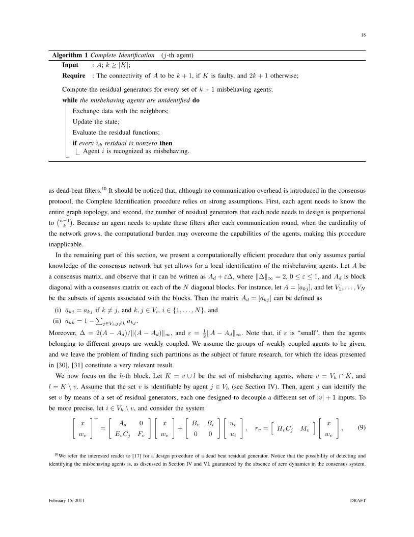
Algorithm 1 Complete Identification (j-th agent)Input : A; k ≥ |K|;Require : The connectivity of A to be k + 1, if K is faulty, and 2k + 1 otherwise;

Compute the residual generators for every set of k + 1 misbehaving agents;

while the misbehaving agents are unidentified doExchange data with the neighbors;

Update the state;

Evaluate the residual functions;

if every ith residual is nonzero thenAgent i is recognized as misbehaving.

as dead-beat filters.10 It should be noticed that, although no communication overhead is introduced in the consensus

protocol, the Complete Identification procedure relies on strong assumptions. First, each agent needs to know the

entire graph topology, and second, the number of residual generators that each node needs to design is proportional

to(n−1

k

). Because an agent needs to update these filters after each communication round, when the cardinality of

the network grows, the computational burden may overcome the capabilities of the agents, making this procedure

inapplicable.

In the remaining part of this section, we present a computationally efficient procedure that only assumes partial

knowledge of the consensus network but yet allows for a local identification of the misbehaving agents. Let A be

a consensus matrix, and observe that it can be written as Ad + ε∆, where ‖∆‖∞ = 2, 0 ≤ ε ≤ 1, and Ad is block

diagonal with a consensus matrix on each of the N diagonal blocks. For instance, let A = [akj ], and let V1, . . . , VN

be the subsets of agents associated with the blocks. Then the matrix Ad = [akj ] can be defined as

(i) akj = akj if k 6= j, and k, j ∈ Vi, i ∈ {1, . . . , N}, and

(ii) akk = 1−∑

j∈Vi,j 6=k akj .

Moreover, ∆ = 2(A − Ad)/‖(A − Ad)‖∞, and ε = 12‖A − Ad‖∞. Note that, if ε is “small”, then the agents

belonging to different groups are weakly coupled. We assume the groups of weakly coupled agents to be given,

and we leave the problem of finding such partitions as the subject of future research, for which the ideas presented

in [30], [31] constitute a very relevant result.

We now focus on the h-th block. Let K = v ∪ l be the set of misbehaving agents, where v = Vh ∩ K, and

l = K \ v. Assume that the set v is identifiable by agent j ∈ Vh (see Section IV). Then, agent j can identify the

set v by means of a set of residual generators, each one designed to decouple a different set of |v|+ 1 inputs. To

be more precise, let i ∈ Vh \ v, and consider the system[x

wv

]+

=

[Ad 0

EvCj Fv

] [x

wv

]+

[Bv Bi

0 0

] [uv

ui

], rv =

[HvCj Mv

] [x

wv

], (9)

10We refer the interested reader to [17] for a design procedure of a dead beat residual generator. Notice that the possibility of detecting andidentifying the misbehaving agents is, as discussed in Section IV and VI, guaranteed by the absence of zero dynamics in the consensus system.


19

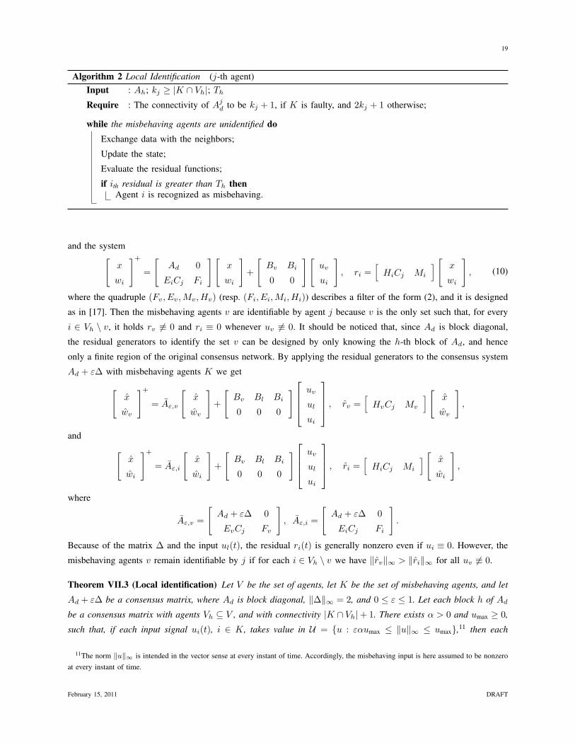
Algorithm 2 Local Identification (j-th agent)Input : Ah; kj ≥ |K ∩ Vh|; Th

Require : The connectivity of Ajd to be kj + 1, if K is faulty, and 2kj + 1 otherwise;

while the misbehaving agents are unidentified doExchange data with the neighbors;

Update the state;

Evaluate the residual functions;

if ith residual is greater than Th thenAgent i is recognized as misbehaving.

and the system[x

wi

]+

=

[Ad 0

EiCj Fi

] [x

wi

]+

[Bv Bi

0 0

] [uv

ui

], ri =

[HiCj Mi

] [x

wi

], (10)

where the quadruple (Fv, Ev,Mv,Hv) (resp. (Fi, Ei,Mi,Hi)) describes a filter of the form (2), and it is designed

as in [17]. Then the misbehaving agents v are identifiable by agent j because v is the only set such that, for every

i ∈ Vh \ v, it holds rv 6≡ 0 and ri ≡ 0 whenever uv 6≡ 0. It should be noticed that, since Ad is block diagonal,

the residual generators to identify the set v can be designed by only knowing the h-th block of Ad, and hence

only a finite region of the original consensus network. By applying the residual generators to the consensus system

Ad + ε∆ with misbehaving agents K we get[x

wv

]+

= Aε,v

[x

wv

]+

[Bv Bl Bi

0 0 0

] uv

ul

ui

, rv =[

HvCj Mv

] [x

wv

],

and [x

wi

]+

= Aε,i

[x

wi

]+

[Bv Bl Bi

0 0 0

] uv

ul

ui

, ri =[

HiCj Mi

] [x

wi

],

where

Aε,v =

[Ad + ε∆ 0

EvCj Fv

], Aε,i =

[Ad + ε∆ 0

EiCj Fi

].

Because of the matrix ∆ and the input ul(t), the residual ri(t) is generally nonzero even if ui ≡ 0. However, the

misbehaving agents v remain identifiable by j if for each i ∈ Vh \ v we have ‖rv‖∞ > ‖ri‖∞ for all uv 6≡ 0.

Theorem VII.3 (Local identification) Let V be the set of agents, let K be the set of misbehaving agents, and let

Ad + ε∆ be a consensus matrix, where Ad is block diagonal, ‖∆‖∞ = 2, and 0 ≤ ε ≤ 1. Let each block h of Ad

be a consensus matrix with agents Vh ⊆ V , and with connectivity |K ∩ Vh|+ 1. There exists α > 0 and umax ≥ 0,

such that, if each input signal ui(t), i ∈ K, takes value in U = {u : εαumax ≤ ‖u‖∞ ≤ umax},11 then each

11The norm ‖u‖∞ is intended in the vector sense at every instant of time. Accordingly, the misbehaving input is here assumed to be nonzeroat every instant of time.


20

well-behaving agent j ∈ Vh identifies in finite time the faulty agents K ∩ Vh by means of the Local Identification

algorithm.

Proof: We focus on the agent j ∈ Vh, and, without loss of generality, we assume that uK(0) 6= 0, and that

the residual generators have a finite impulse response. Let dj = ‖Vh‖, and note that dj time steps are sufficient

for each agent j ∈ Vh to identify the misbehaving agents. Let ut denote the input sequence up to time t. Let

v = K ∩ Vh, l = K \ v, and observe that rv(dj) = [ HvCj Mv ] Adjε,vx(0) + hv ? u

dj−1v + hl ? u

dj−1l , where hv

and hl denote the impulse response from uv and ul respectively, and ? denotes the convolution operator. We

now determine an upper bound for each term of rv(dj). Let the misbehaving inputs take value in U = {u :

εαumax ≤ ‖u‖∞ ≤ umax}. By using the triangle inequality on the impulse responses of the residual generator,

it can be shown that ‖hl ? udj−1l ‖∞ ≤ ‖hl ? u

dj−1l ‖∞ + εc1umax = εc1umax, where hl denotes the impulse

response form ul to rv of the system (9), and c1 is a finite positive constant independent of ε. Moreover, it can

be shown that there exist two positive constant c2 and c3 such that ‖ [ HvCj Mv ] Adjε,vx(0)‖∞ ≤ εc2umax, and

minuv∈U ‖hv ? udj−1v ‖∞ ≥ minuv∈U ‖hv ? u

dj−1v ‖∞ − εc3umax. Analogously, for the residual generator associated

with the well-behaving agent i, we have ri(dj) = [ HiCj Mi ] Adj

ε,ix(0) + hv ? udj−1v + hl ? u

dj−1l , and hence

ri(dj) ≤ ε(c(i)4 + c

(i)5 + c

(i)6 )umax. Let c = c1 + c2 + c3 + maxi∈Vh\v(c(i)

4 + c(i)5 + c

(i)6 ), and let β be such

that minuv∈U ‖hv ? udj−1v ‖∞ > βumin. Then a correct identification of the misbehaving agents v takes place if

βumin = βεαumax > εcumax, and hence if α > c/β.

Notice that the constant α in Theorem VII.3 can be computed by bounding the infinity norm of the impulse

response of the residual generators. An example is in Section VIII-B. A procedure to achieve local detection

and identification of misbehaving agents is in Algorithm 2, where Ahd denotes the h-th block of Ad, and Th the

corresponding threshold value. Observe that in the Local Identification procedure an agent only performs local

computation, and it is assumed to have only local knowledge of the network structure.

Remark 3 It is not a trivial fact that the misbehaving agents become locally identifiable when the parameter ε is

sufficiently small. Indeed, as long as ε > 0, the effect of the perturbation ε∆ on the residuals becomes eventually

relevant with respect to the dynamics described by only Ad, preventing, after a certain time, a correct identification

of the misbehaving agents [30].

VIII. EXAMPLES

In the first example of this section the Complete Identification algorithm is used, while in the second example

the Local Identification procedure is implemented.

A. Complete detection and identification

Consider the network of Fig. 3(a), and let A be a randomly chosen consensus matrix. In particular,

A =

0.2795 0.1628 0 0.1512 0.4066 0 0 00.0143 0.3363 0.3469 0 0 0.3025 0 0

0 0.0718 0.1904 0.2438 0 0 0.4941 00.0844 0 0.4457 0.0660 0 0 0 0.40400.1709 0 0 0 0.2694 0.2472 0 0.3125

0 0.4199 0 0 0.1575 0.3293 0.0932 00 0 0.0174 0 0 0.4241 0.2850 0.27350 0 0 0.3024 0.2039 0 0.2065 0.2873

.

The network is 3-connected, and it can be verified that for any set K of 3 misbehaving agents, and for any observer

node j, the triple (A,BK , Cj) is left-invertible. Also, for any set K of cardinality 2, and for any node j, the triple

(A,BK , Cj) has no invariant zeros. As previously discussed, any well-behaving node can detect and identify up to 2


21

1

65

8 7

34

2

(a)

! " # $ % & ' ( ) !* !! !"

*

*+!

*+"

*+#

*+$

,-./

0

0

! " # $ % & ' ( ) !* !! !"

!*+!

!*+*%

*

*+*%

,-./

0

0

! " # $ % & ' ( ) !* !! !"

!*+"

!*+!

*

*+!

*+"

,-./

0

0

3-th residual

4-th residual

7-th residual

(b)

Fig. 3. In Fig. 3(a) a consensus network where the nodes 3 and 7 are faulty. In Fig. 3(b) the residual functions computed by the agent 1 underthe hypothesis that the misbehaving set is {3, 4, 7}.

faulty agents, or up to 1 malicious agent. Consider the observations of the agent 1, and suppose that the agents {3, 7}inject a random signal into the network. As described in Algorithm 1, the agent 1 designs the residual generator

filters and computes the residual functions for each of the(73

)possible sets of misbehaving nodes, and identify the

well-behaving agents. Consider for example the system x(t + 1) = Ax(t) + B3u3(t) + B4u4(t) + B7u7(t), and

suppose we want to design a filter of the form (2) which is only sensible to the signal u4. The unobservability

subspace SM{3,7} = (V∗{3,7} + S∗{3,7}), is

SM{3,7} = Im

0 0 0 0 00 0 0 −0.6624 00 1 0 0 00 0 −0.4740 −0.6597 00 0 −0.8798 0.3548 0

0.4116 0 −0.0327 0.0132 00 0 0 0 1

0.9114 0 0.0148 −0.0060 0

,

and a possible choice for the matrices of the residual generator is

F =[

0 0 00.0014 −0.3222 −0.3424−0.0013 0.3031 0.3222

], E =

[0.2795 0.1628 0.1512 0.40660.0138 0.4982 −0.2280 0.20030.0082 −0.6095 0.3012 −0.1568

],

M =[−1 0 0

0 0.9999 0.0128

], H =

[1 0 0 00 −0.7491 0.5832 −0.3142

].

It can be checked that, independent of the initial condition of the network, the residual function associated with

the input 4 is zero, as in 3(b), so that the agent 4 is regarded as well-behaving. Agents 3, 7, instead, have always

nonzero residual functions, and are recognized as misbehaving. If the misbehaving nodes are allowed to be malicious,

then no more than 1 misbehaving node can be tolerated. Indeed, because of Theorem IV.1, there exists a set K

of 4 misbehaving agents such that the system (A,BK , C1) exhibits nontrivial zero dynamics. For instance, let

K = {2, 4, 6, 8}, and note that if the initial condition x(0) belongs to

V∗ = Im

0 0 00 0 01 0 00 0 00 0 00 0.7842 00 0 10 −0.6205 0

,

then the input uK(t) = Fbx(t), where

Fb =[ 0 0 −0.3469 0 0 −0.1860 0 0.1472

0 0 −0.4457 0 0 0.1966 0 −0.15550 0 0 0 0 −0.1063 −0.1148 0.08410 0 0 0 0 0.0636 −0.1894 −0.0503

],


22

1

5

6

4

7

2

3ε

ε

(a)

0 0.01 0.02 0.03 0.04 0.05 0.06 0.070

0.05

0.1

0.15

ε∗

(b)

Fig. 4. In Fig. 4(a) a consensus network with weak connections. In Fig. 4(b) the solid line corresponds to the largest magnitude of the residualassociated with the well-behaving agent 3, while the dashed line denotes the smallest magnitude of the residual associated with the misbehavingagent 2, both as a function of the parameter ε. If ε ≤ ε∗, then there exists a threshold that allows to identify the misbehaving agent 2.

is such that y1(t) = 0 for all t ≥ 0.12 Therefore, the two systems (A,B{2,4}, C1) and (A,B{6,8}, C1), with initial

conditions x1(0) and x2(0) = x1(0)− x(0), and inputs

u{2,4}(t) = [ 1 0 0 00 1 0 0 ]Fb(x1(t)− x2(t)), u{6,8}(t) = [ 0 0 1 0

0 0 0 1 ]Fb(x2(t)− x1(t)),

have exactly the same output dynamic, so that the two sets {2, 4} and {6, 8} are indistinguishable by the agent 1.

B. Local detection and identification

Consider the consensus network in Fig. 4(a), where A = Ad + ε∆, and

Ad =

1/3 1/3 1/3 0 0 0 01/3 1/3 1/3 0 0 0 01/3 1/3 1/3 0 0 0 00 0 0 1/4 1/4 1/4 1/40 0 0 1/4 1/4 1/4 1/40 0 0 1/4 1/4 1/4 1/40 0 0 1/4 1/4 1/4 1/4

, ∆ =

0 0 0 0 0 0 00 −1 0 1 0 0 00 0 −1 0 0 0 10 0 1 0 −1 0 00 0 0 0 0 0 00 0 0 0 0 0 00 0 1 0 0 0 −1

.

Let K = {2, 7} be the set of misbehaving agents, let 0.1 ≤ u2(t), u7(t) ≤ 3 at each time t, and let ‖x(0)‖∞ ≤ 1.

Consider the agent 1, and let (F2, E2,M2,H2) and (F3, E3,M3,H3) be the residual generators as in (9) and (10)

respectively, where

F2 =[−1/3 −1/31/3 1/3

], E2 =

[−2/3 0 −1/32/3 0 1/3

], M2 =

[1 00 −1

], H2 = [ 1 0 0

0 1 0 ] ,

and

F3 =[−1/3 1/3−1/3 1/3

], E3 =

[−2/3 −1/3 0−2/3 −1/3 0

], M3 =

[−1 00 1

], H3 =

[−1 0 00 0 1

].

Let h32 (resp. h3

7) be the impulse response from the input u2 (resp. u7) to r3, and let u12 (resp. u1

7) denote the input

signal u2 (resp. u7) up to time 1. Note that the misbehaving agent can be identified after 2 time steps, and that the

residual associated with the agent 3 is

r3(2) = [ H3C1 M3 ][

Ad+ε∆ 0E3C1 F3

]2 [x(0)

0

]+ h3

2 ? u12 + h3

7 ? u17,

where ? denotes the convolution operator. After some computation we obtain

r3(2) = ε [ H3C1 M3 ][

Ad∆+∆Ad+ε∆2 ∆B2 ∆B7E3C1∆ 0 0

] [x(0)u2(0)u7(0)

]

12Notice that the malicious agents need to know the entire state to implement this feedback law. The case in which the malicious agents canonly implement local feedback actions is left as a direction for future research, for which the result in [12] is very relevant.


23

(a)

0 0.005 0.01 0.015 0.02 0.025 0.03 0.035 0.04 0.045 0.050

0.05

0.1

0.15

0.2

0.25

(b)

Fig. 5. In Fig. 5(a) a consensus network partitioned into 3 areas. Each agent identifies the neighboring misbehaving agents by only knowingthe topology of the subnetwork it belongs to. In Fig. 5(b) the smallest magnitude of the residual associated with a misbehaving agent (dashedline) and the largest magnitude of the residual associated with a well-behaving agent (solid line) are plotted as a function of ε.

and, analogously,

r2(2) = ε [ H2C1 M2 ][

Ad∆+∆Ad+ε∆2 ∆B2 ∆B7E2C1∆ 0 0

] [x(0)u2(0)u7(0)

]+ [ H2C1 M2 ]

[AdB2 B2

E2C1B2 0

] [u2(0)u2(1)

]Recall that the agent 1 is able to identify the misbehaving agent 2 if, independent of u1

2 and u17, there exists a

threshold T such that ‖r2(2)‖∞ ≥ T , and ‖r3(2)‖∞ < T . The behavior of ‖r2(2)‖∞ and ‖r3(2)‖∞ as a function

of ε is in Fig. 4(b). Note that for ε = ε∗ = 0.026 we have ‖r2(2)‖∞ = ‖r3(2)‖∞ = 0.07. For instance, if ε = 0.01,

then it can be verified that ‖r2(2)‖∞ > 0.1, and ‖r3(2)‖∞ < 0.05. It follows that a threshold T = 0.1 allows

the agent 1 to identify the misbehaving agent 2. On the other hand, if ε = 0.03, then ‖r2(2)‖∞ ≥ 0.01, and

‖r3(2)‖∞ ≤ 0.12, so that the misbehaving agent 2 may remain unidentified. Indeed, if x(0) = [ 1 1 1 −1 −1 −1 −1 ],

u12 = u1

7 = [ 0.1 0.1 ], then ‖r2(2)‖∞ = 0.01 and ‖r3(2)‖∞ = 0.12, so that the agent 3 is recognized as misbehaving

instead of the agent 2.

As a final remark, note that the larger the consensus network, the more convenient the proposed approximation

procedure becomes. For instance, consider the network presented in [32], and here reported in Fig. 5(a). Such

a clustered interconnection structure, in which the edges connecting different clusters have a small weight, may

be preferable in many applications because much simpler and efficient protocols can be implemented within each

cluster. Assume that there is a misbehaving agent in each cluster, and consider the residuals computed after 5 steps

of the consensus algorithm. Let ε be the weight of the edges connecting different clusters. Fig. 5(b) shows, as a

function of ε, the smallest magnitude of the residual associated with a misbehaving agent (dashed line) versus the

largest magnitude of the residual associated with a well-behaving agent (solid line). If ε is sufficiently small, then

our local identification method allows each well-behaving agent to promptly detect and identify the misbehaving

agents belonging to the same group, and hence to restore the functionality of the network. For instance, if ε ≤ 0.01,

then, following Theorem VII.3, if the misbehaving input take value in {u : 0.1 ≤ |u| ≤ 3}, then a misbehaving

agent is correctly detected and identified by a well-behaving agent.

IX. CONCLUSION

The problem of distributed reliable computation in networks with misbehaving nodes is considered, and its

relationship with the fault detection and isolation problem for linear systems is discussed. The resilience of linear

consensus networks to external attacks is characterized through some properties of the underlying communication


24

graph, as well as from a system-theoretic perspective. In almost any linear consensus network, the misbehaving

components can be correctly detected and identified, as long as the connectivity of the communication graph

is sufficiently high. Precisely, for a linear distributed consensus network to be resilient to k concurrent faults, the

connectivity of the communication graph needs to be 2k+1, if Byzantine failures are allowed, and k+1, otherwise.

Finally, for the faulty agents case, good performance can be obtained even when the agents do not know the entire

topology of the consensus network, or when they are subject to memory or computation constraints.

Interesting aspects requiring further investigation include a quantitative study of the strong observability of a

consensus network. More precisely, instead of determining whether or not a consensus network is strongly observable

from the agent j, it is useful to characterize the gain between the inputs of a set of misbehaving agents and the

observations of the agent j. Indeed, depending on how small such gain is, some undetectable behaviors may be

neglected because not implementable by the misbehaving agents. Additionally, it is of interest to study the strong

observability property under specific consensus protocols, e.g., those resulting from an optimization process on

the communication weights, or those preserving the statistical properties of the initial consensus vector. Finally,

the problem of clustering a large network into smaller parts is crucial for the performance of the proposed local

identification procedure, and it remains the subject of future research.

REFERENCES

[1] W. Ren, R. W. Beard, and E. M. Atkins, “Information consensus in multivehicle cooperative control: Collective group behavior throughlocal interaction,” IEEE Control Systems Magazine, vol. 27, no. 2, pp. 71–82, 2007.

[2] R. Olfati-Saber, J. A. Fax, and R. M. Murray, “Consensus and cooperation in networked multi-agent systems,” Proceedings of the IEEE,vol. 95, no. 1, pp. 215–233, 2007.

[3] F. Bullo, J. Cortes, and S. Martınez, Distributed Control of Robotic Networks, ser. Applied Mathematics Series. Princeton UniversityPress, 2009, available at http://www.coordinationbook.info.

[4] N. A. Lynch, Distributed Algorithms. Morgan Kaufmann, 1997.[5] A. Jadbabaie, J. Lin, and A. S. Morse, “Coordination of groups of mobile autonomous agents using nearest neighbor rules,” IEEE

Transactions on Automatic Control, vol. 48, no. 6, pp. 988–1001, 2003.[6] R. Olfati-Saber and R. M. Murray, “Consensus problems in networks of agents with switching topology and time-delays,” IEEE Transactions

on Automatic Control, vol. 49, no. 9, pp. 1520–1533, 2004.[7] L. Xiao and S. Boyd, “Fast linear iterations for distributed averaging,” Systems & Control Letters, vol. 53, pp. 65–78, 2004.[8] P. Michiardi and R. Molva, “CORE: A collaborative reputation mechanism to enforce node cooperation in mobile ad hoc network,” in

Communications and Multimedia Security Conference (CMS), Portoroz, Slovenia, Sept. 2002.[9] L. Lamport, R. Shostak, and M. Pease, “The Byzantine generals problem,” ACM Transactions on Programming Languages and Systems,

vol. 4, no. 3, pp. 382–401, 1982.[10] D. Dolev, “The Byzantine generals strike again,” Journal of Algorithms, vol. 3, pp. 14–30, 1982.[11] F. Pasqualetti, A. Bicchi, and F. Bullo, “Distributed intrusion detection for secure consensus computations,” in IEEE Conf. on Decision

and Control, New Orleans, LA, Dec. 2007, pp. 5594–5599.[12] S. Sundaram and C. N. Hadjicostis, “Distributed function calculation via linear iterations in the presence of malicious agents - Part I:

Attacking the network,” in American Control Conference, Seattle, WA, June 2008, pp. 1350–1355.[13] ——, “Distributed function calculation via linear iterations in the presence of malicious - Part II: Overcoming malicious behavior,” in

American Control Conference, Seattle, WA, June 2008, pp. 1356–1361.[14] R. Patton, P. Frank, and R. Clark, Fault Diagnosis in Dynamic Systems: Theory and Applications. Prentice Hall, 1989.[15] G. Basile and G. Marro, Controlled and Conditioned Invariants in Linear System Theory. Prentice Hall, 1991.[16] W. M. Wonham, Linear Multivariable Control: A Geometric Approach, 3rd ed. Springer, 1985.[17] M.-A. Massoumnia, G. C. Verghese, and A. S. Willsky, “Failure detection and identification,” IEEE Transactions on Automatic Control,

vol. 34, no. 3, pp. 316–321, 1989.[18] C. D. Godsil and G. F. Royle, Algebraic Graph Theory, ser. Graduate Texts in Mathematics. Springer, 2001, vol. 207.[19] C. D. Meyer, Matrix Analysis and Applied Linear Algebra. SIAM, 2001.[20] R. A. Horn and C. R. Johnson, Matrix Analysis. Cambridge University Press, 1985.


25

[21] H. L. Trentelman, A. Stoorvogel, and M. Hautus, Control Theory for Linear Systems. Springer, 2001.[22] J. Tokarzewski, Finite Zeros in Discrete Time Control Systems, ser. Lecture notes in control and information sciences. Springer, 2006.[23] E. Montijano, S. Martınez, and S. Sagues, “De-ransac: Robust distributed consensus in sensor networks,” IEEE Transactions on Systems,

Man & Cybernetics. Part B: Cybernetics, May 2010, submitted.[24] J. M. Dion, C. Commault, and J. van der Woude, “Generic properties and control of linear structured systems: a survey,” Automatica,

vol. 39, no. 7, pp. 1125–1144, 2003.[25] K. J. Reinschke, Multivariable Control: A Graph-Theoretic Approach. Springer, 1988.[26] J. van der Woude, “The generic number of invariant zeros of a structured linear system,” SIAM Journal on Control and Optimization,

vol. 38, no. 1, pp. 1–21, 1999.[27] A. N. Kolmogorov and S. V. Fomin, Introductory Real Analysis. Dover Publications, 1975.[28] K. Tchon, “On generic properties of linear systems: An overview,” Kybernetika, vol. 19, no. 6, pp. 467–474, 1983.[29] H. Minc, Nonnegative Matrices. Wiley, 1988.[30] R. G. Phillips and P. Kokotovic, “A singular perturbation approach to modeling and control of Markov chains,” IEEE Transactions on

Automatic Control, vol. 26, no. 5, pp. 1087–1094, 1981.[31] J. H. Chow, J. Cullum, and R. A. Willoughby, “A sparsity-based technique for identifying slow-coherent areas in large power systems,”

IEEE Transactions on Power Apparatus and Systems, vol. PAS-103, no. 3, pp. 463–473, 1984.[32] E. Bıyık and M. Arcak, “Area aggregation and time-scale modeling for sparse nonlinear networks,” Systems & Control Letters, vol. 57,

no. 2, pp. 142–149, 2007.


1 Consensus Computation in Unreliable Networks: A System ...

Documents

Transcript of 1 Consensus Computation in Unreliable Networks: A System ...