1

Clustering

Sunita Sarawagi

http://www.it.iitb.ac.in/~sunita

Outline

What is Clustering Similarity measures Clustering Methods Summary References

What Is Good Clustering?

A good clustering method will produce high quality clusters with high intra-class similarity low inter-class similarity

The quality of a clustering result depends on both the similarity measure used by the method and its implementation.

The quality of a clustering method is also measured by its ability to discover some or all of the hidden patterns.

Chapter 8. Cluster Analysis

What is Cluster Analysis? Types of Data in Cluster Analysis A Categorization of Major Clustering Methods Partitioning Methods Hierarchical Methods Density-Based Methods Grid-Based Methods Model-Based Clustering Methods Outlier Analysis Summary

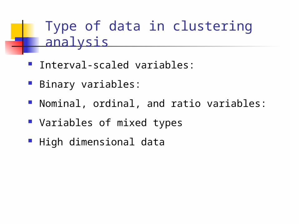
Type of data in clustering analysis

Interval-scaled variables:

Binary variables:

Nominal, ordinal, and ratio variables:

Variables of mixed types

High dimensional data

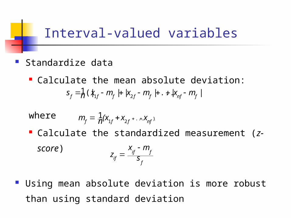
Interval-valued variables

Standardize data

Calculate the mean absolute deviation:

where

Calculate the standardized measurement (z-

score)

Using mean absolute deviation is more robust than

using standard deviation

.)...21

1nffff

xx(xn m

|)|...|||(|121 fnffffff

mxmxmxns

f

fifif s

mx z

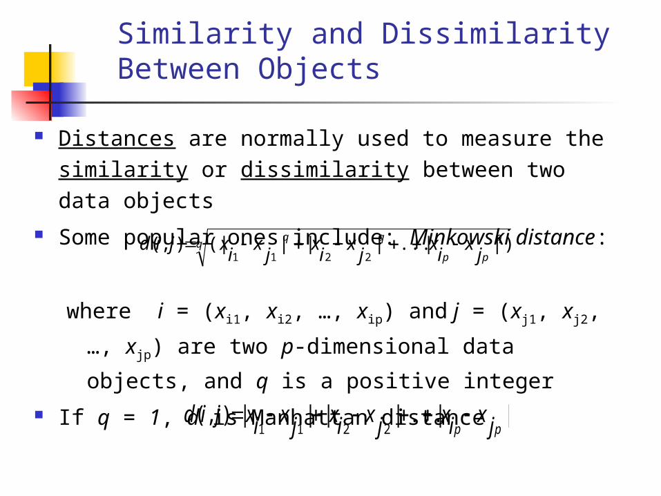
Similarity and Dissimilarity Between Objects

Distances are normally used to measure the similarity or dissimilarity between two data objects

Some popular ones include: Minkowski distance:

where i = (xi1, xi2, …, xip) and j = (xj1, xj2, …, xjp)

are two p-dimensional data objects, and q is a positive integer

If q = 1, d is Manhattan distance

qq

pp

qq

jx

ix

jx

ix

jx

ixjid )||...|||(|),(

2211

||...||||),(2211 pp jxixjxixjxixjid

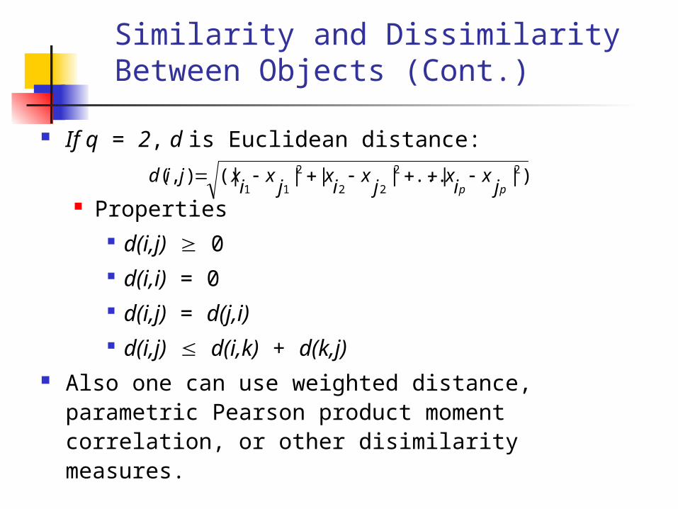
Similarity and Dissimilarity Between Objects (Cont.)

If q = 2, d is Euclidean distance:

Properties d(i,j) 0 d(i,i) = 0 d(i,j) = d(j,i) d(i,j) d(i,k) + d(k,j)

Also one can use weighted distance, parametric Pearson product moment correlation, or other disimilarity measures.

)||...|||(|),( 22

22

2

11 pp jx

ix

jx

ix

jx

ixjid

Binary Variables

A contingency table for binary data

Simple matching coefficient (invariant, if the

binary variable is symmetric):

Jaccard coefficient (noninvariant if the binary

variable is asymmetric):

dcbacb jid

),(

pdbcasum

dcdc

baba

sum

0

1

01

cbacb jid

),(

Object i

Object j

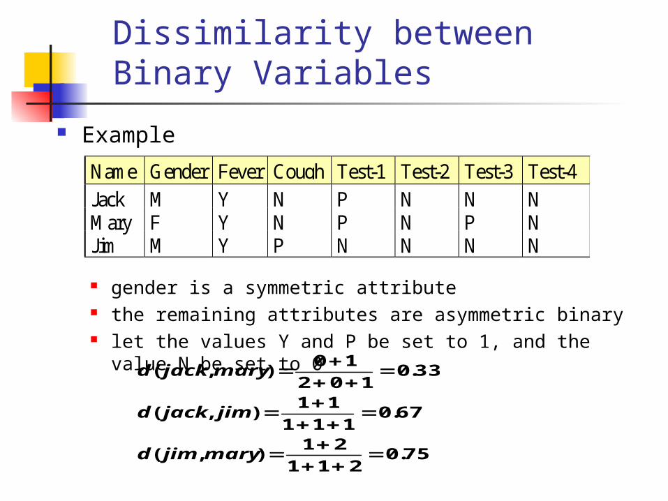
Dissimilarity between Binary Variables

Example

gender is a symmetric attribute the remaining attributes are asymmetric binary let the values Y and P be set to 1, and the value N be

set to 0

Name Gender Fever Cough Test-1 Test-2 Test-3 Test-4

Jack M Y N P N N NMary F Y N P N P NJim M Y P N N N N

75.0211

21),(

67.0111

11),(

33.0102

10),(

maryjimd

jimjackd

maryjackd

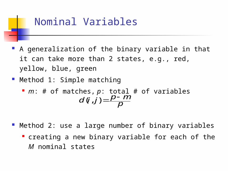
Nominal Variables

A generalization of the binary variable in that it can take more than 2 states, e.g., red, yellow, blue, green

Method 1: Simple matching m: # of matches, p: total # of variables

Method 2: use a large number of binary variables creating a new binary variable for each of the M

nominal states

pmpjid ),(

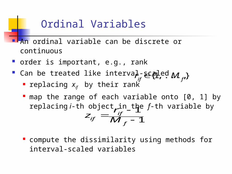
Ordinal Variables

An ordinal variable can be discrete or continuous order is important, e.g., rank Can be treated like interval-scaled

replacing xif by their rank

map the range of each variable onto [0, 1] by replacing i-th object in the f-th variable by

compute the dissimilarity using methods for interval-scaled variables

11

f

ifif M

rz

},...,1{fif

Mr

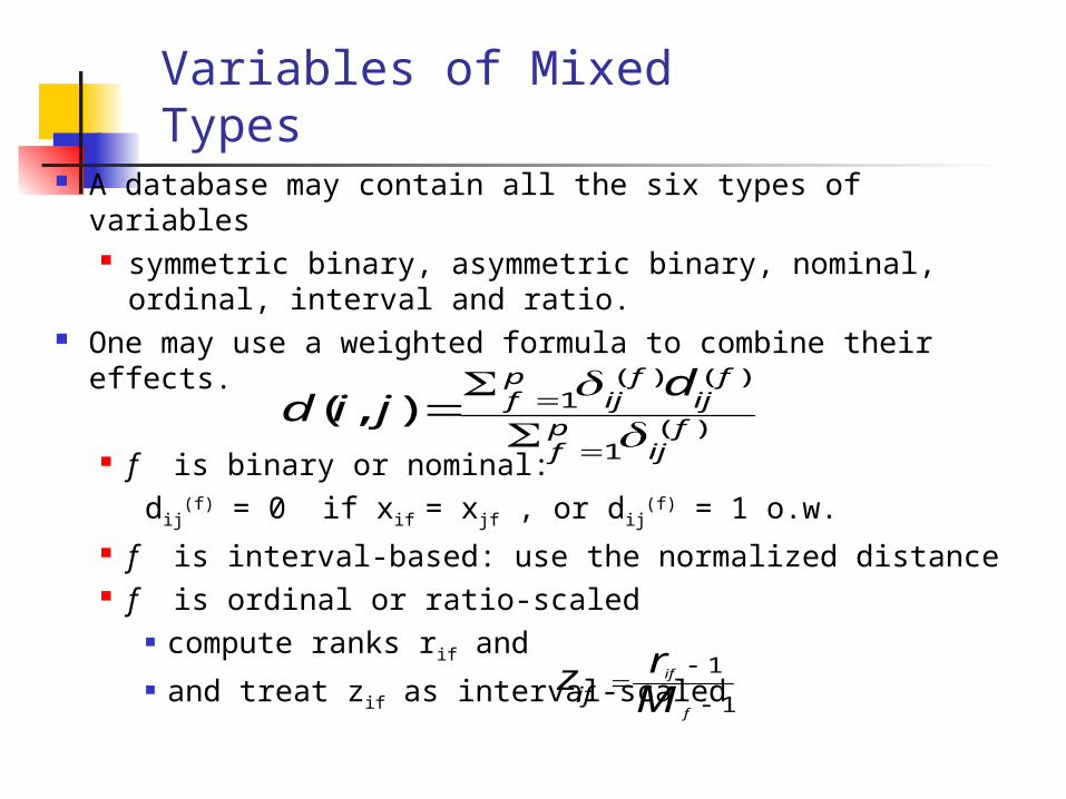
Variables of Mixed Types

A database may contain all the six types of variables symmetric binary, asymmetric binary, nominal,

ordinal, interval and ratio. One may use a weighted formula to combine their

effects.

f is binary or nominal:dij

(f) = 0 if xif = xjf , or dij(f) = 1 o.w.

f is interval-based: use the normalized distance f is ordinal or ratio-scaled

compute ranks rif and and treat zif as interval-scaled

)(1

)()(1),(

fij

pf

fij

fij

pf

djid

1

1

f

if

Mrz

if

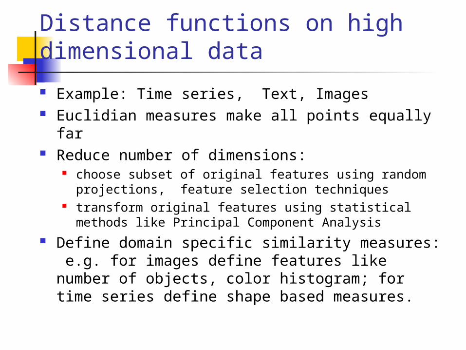
Distance functions on high dimensional data

Example: Time series, Text, Images Euclidian measures make all points equally far Reduce number of dimensions:

choose subset of original features using random projections, feature selection techniques

transform original features using statistical methods like Principal Component Analysis

Define domain specific similarity measures: e.g. for images define features like number of objects, color histogram; for time series define shape based measures.

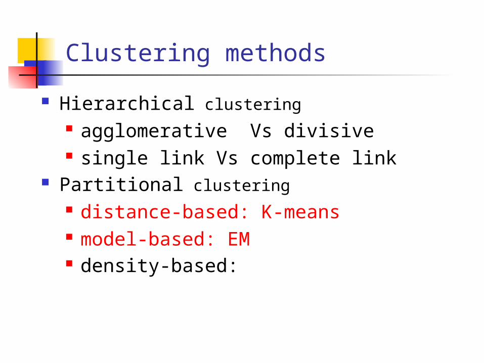
Clustering methods

Hierarchical clustering agglomerative Vs divisive single link Vs complete link

Partitional clustering distance-based: K-means model-based: EM density-based:

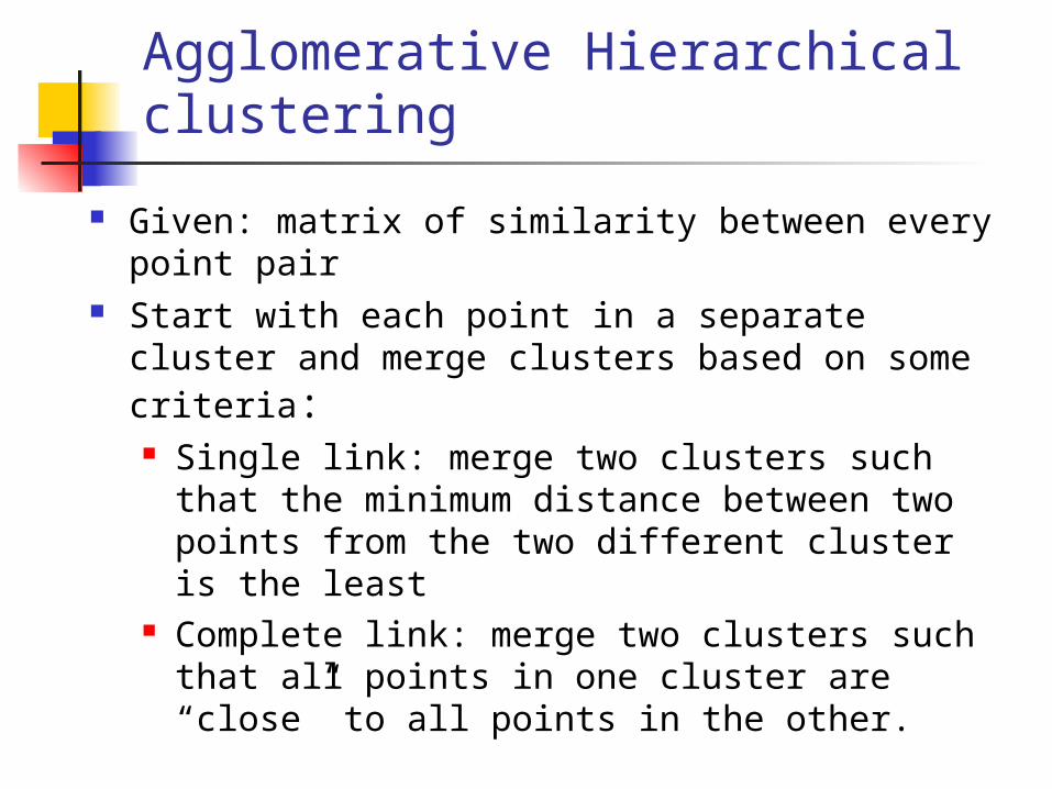
Agglomerative Hierarchical clustering

Given: matrix of similarity between every point pair

Start with each point in a separate cluster and merge clusters based on some criteria: Single link: merge two clusters such that the

minimum distance between two points from the two different cluster is the least

Complete link: merge two clusters such that all points in one cluster are “close” to all points in the other.

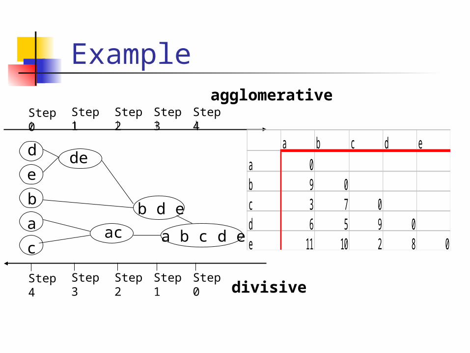
Example

Step 0 Step 1 Step 2 Step 3 Step 4

e

a

b

c

d de

ac

b d e

a b c d e

Step 4 Step 3 Step 2 Step 1 Step 0

agglomerative

divisive

a b c d e

a 0b 9 0c 3 7 0d 6 5 9 0e 11 10 2 8 0

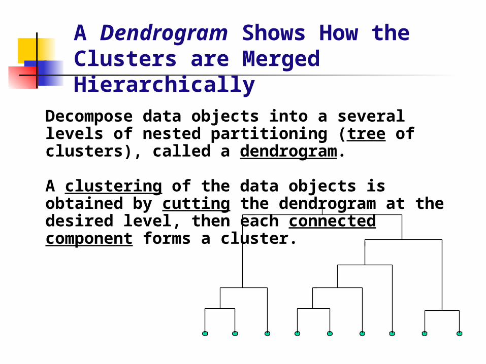
A Dendrogram Shows How the Clusters are Merged Hierarchically

Decompose data objects into a several levels of nested partitioning (tree of clusters), called a dendrogram.

A clustering of the data objects is obtained by cutting the dendrogram at the desired level, then each connected component forms a cluster.

Partitioning Algorithms: Basic Concept

Partitioning method: Construct a partition of a database D of n objects into a set of k clusters

Given a k, find a partition of k clusters that optimizes the chosen partitioning criterion Global optimal: exhaustively enumerate all partitions Heuristic methods: k-means and k-medoids

algorithms k-means (MacQueen’67): Each cluster is represented

by the center of the cluster k-medoids or PAM (Partition around medoids)

(Kaufman & Rousseeuw’87): Each cluster is represented by one of the objects in the cluster

The K-Means Clustering Method

Given k, the k-means algorithm is implemented in 4 steps: Partition objects into k nonempty subsets Compute seed points as the centroids of the

clusters of the current partition. The centroid is the center (mean point) of the cluster.

Assign each object to the cluster with the nearest seed point.

Go back to Step 2, stop when no more new assignment.

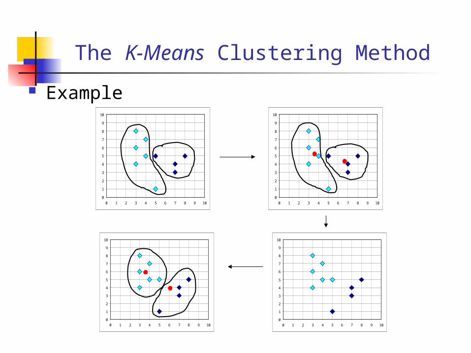
The K-Means Clustering Method

Example

0

1

2

3

4

5

6

7

8

9

10

0 1 2 3 4 5 6 7 8 9 10

0

1

2

3

4

5

6

7

8

9

10

0 1 2 3 4 5 6 7 8 9 10

0

1

2

3

4

5

6

7

8

9

10

0 1 2 3 4 5 6 7 8 9 10

0

1

2

3

4

5

6

7

8

9

10

0 1 2 3 4 5 6 7 8 9 10

Comments on the K-Means Method

Strength Relatively efficient: O(tkn), where n is # objects, k is #

clusters, and t is # iterations. Normally, k, t << n. Often terminates at a local optimum. The global

optimum may be found using techniques such as: deterministic annealing and genetic algorithms

Weakness Applicable only when mean is defined, then what about

categorical data? Need to specify k, the number of clusters, in advance Unable to handle noisy data and outliers Not suitable to discover clusters with non-convex

shapes

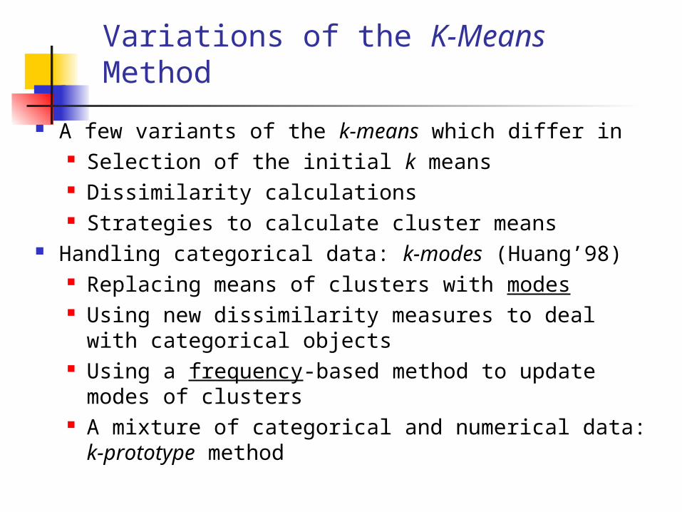
Variations of the K-Means Method

A few variants of the k-means which differ in Selection of the initial k means Dissimilarity calculations Strategies to calculate cluster means

Handling categorical data: k-modes (Huang’98) Replacing means of clusters with modes Using new dissimilarity measures to deal with

categorical objects Using a frequency-based method to update modes

of clusters A mixture of categorical and numerical data: k-

prototype method

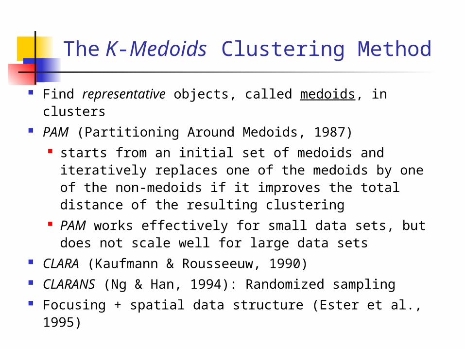
The K-Medoids Clustering Method

Find representative objects, called medoids, in clusters

PAM (Partitioning Around Medoids, 1987) starts from an initial set of medoids and

iteratively replaces one of the medoids by one of the non-medoids if it improves the total distance of the resulting clustering

PAM works effectively for small data sets, but does not scale well for large data sets

CLARA (Kaufmann & Rousseeuw, 1990) CLARANS (Ng & Han, 1994): Randomized sampling Focusing + spatial data structure (Ester et al., 1995)

Model based clustering

Assume data generated from K probability distributions

Typically Gaussian distribution Soft or probabilistic version of K-means clustering

Need to find distribution parameters. EM Algorithm

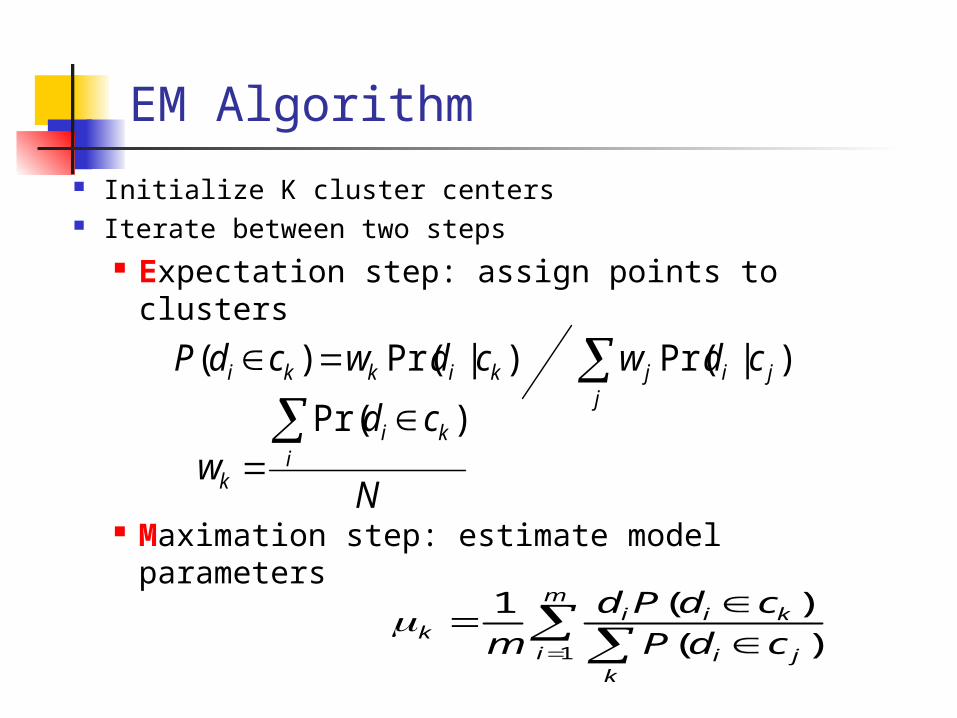
EM Algorithm

Initialize K cluster centers Iterate between two steps

Expectation step: assign points to clusters

Maximation step: estimate model parameters

j

jijkikki cdwcdwcdP ) |Pr() |Pr() (

m

ik

ji

kiik cdP

cdPd

m 1 ) (

) (1

N

cdw i

ki

k

) Pr(

Summary

Cluster analysis groups objects based on their similarity and has wide applications

Measure of similarity can be computed for various types of data

Clustering algorithms can be categorized into partitioning methods, hierarchical methods, and model-based methods

Outlier detection and analysis are very useful for fraud detection, etc. and can be performed by statistical, distance-based or deviation-based approaches

Acknowledgements: slides partly from Jiawei Han’s book: Data mining concepts and Techniques.

References (1)

R. Agrawal, J. Gehrke, D. Gunopulos, and P. Raghavan. Automatic subspace clustering of high dimensional data for data mining applications. SIGMOD'98

M. R. Anderberg. Cluster Analysis for Applications. Academic Press, 1973. M. Ankerst, M. Breunig, H.-P. Kriegel, and J. Sander. Optics: Ordering points to

identify the clustering structure, SIGMOD’99. P. Arabie, L. J. Hubert, and G. De Soete. Clustering and Classification. World

Scietific, 1996 M. Ester, H.-P. Kriegel, J. Sander, and X. Xu. A density-based algorithm for

discovering clusters in large spatial databases. KDD'96. M. Ester, H.-P. Kriegel, and X. Xu. Knowledge discovery in large spatial

databases: Focusing techniques for efficient class identification. SSD'95. D. Fisher. Knowledge acquisition via incremental conceptual clustering.

Machine Learning, 2:139-172, 1987. D. Gibson, J. Kleinberg, and P. Raghavan. Clustering categorical data: An

approach based on dynamic systems. In Proc. VLDB’98. S. Guha, R. Rastogi, and K. Shim. Cure: An efficient clustering algorithm for

large databases. SIGMOD'98. A. K. Jain and R. C. Dubes. Algorithms for Clustering Data. Printice Hall, 1988.

References (2)

L. Kaufman and P. J. Rousseeuw. Finding Groups in Data: an Introduction to Cluster Analysis. John Wiley & Sons, 1990.

E. Knorr and R. Ng. Algorithms for mining distance-based outliers in large datasets. VLDB’98.

G. J. McLachlan and K.E. Bkasford. Mixture Models: Inference and Applications to Clustering. John Wiley and Sons, 1988.

P. Michaud. Clustering techniques. Future Generation Computer systems, 13, 1997.

R. Ng and J. Han. Efficient and effective clustering method for spatial data mining. VLDB'94.

E. Schikuta. Grid clustering: An efficient hierarchical clustering method for very large data sets. Proc. 1996 Int. Conf. on Pattern Recognition, 101-105.

G. Sheikholeslami, S. Chatterjee, and A. Zhang. WaveCluster: A multi-resolution clustering approach for very large spatial databases. VLDB’98.

W. Wang, Yang, R. Muntz, STING: A Statistical Information grid Approach to Spatial Data Mining, VLDB’97.

T. Zhang, R. Ramakrishnan, and M. Livny. BIRCH : an efficient data clustering method for very large databases. SIGMOD'96.