1 Classification Methods: k-Nearest Neighbor Naïve Bayes Ram Akella Lecture 4 February 9, 2011 UC...
57
1 Classification Methods: k-Nearest Neighbor Naïve Bayes Ram Akella Lecture 4 February 9, 2011 UC Berkeley Silicon Valley Center/SC
-
date post
19-Dec-2015 -
Category
Documents
-
view
217 -
download
2
Transcript of 1 Classification Methods: k-Nearest Neighbor Naïve Bayes Ram Akella Lecture 4 February 9, 2011 UC...
1
Classification Methods: k-Nearest Neighbor Naïve Bayes
Ram AkellaLecture 4February 9, 2011
UC Berkeley Silicon Valley Center/SC
2
Overview
Example The Naïve rule Two data-driven methods (no model)
K-nearest neighbors Naïve Bayes

3
Example: Personal Loan Offer
As part of customer acquisition efforts, Universal bank wants to run a campaign for current customers to purchase a loan.In order to improve target marketing, they want to find customers that are most likely to accept the personal loan offer.They use data from a previous campaign on 5000 customers, 480 of them accepted.

4
Personal Loan Data Description
ID Customer IDAge Customer's age in completed yearsExperience #years of professional experienceIncome Annual income of the customer ($000)ZIPCode Home Address ZIP code.Family Family size of the customerCCAvg Avg. spending on credit cards per month ($000)Education Education Level. 1: Undergrad; 2: Graduate; 3: Advanced/ProfessionalMortgage Value of house mortgage if any. ($000)Personal Loan Did this customer accept the personal loan offered in the last campaign?Securities Account Does the customer have a securities account with the bank?CD Account Does the customer have a certificate of deposit (CD) account with the bank?Online Does the customer use internet banking facilities?CreditCard Does the customer use a credit card issued by UniversalBank?
File: “UniversalBank KNN NBayes.xls”
5
The Naïve Rule
Classify a new observation as a member of the majority class In the personal loan example, the
majority of customers did not accept the loan

6
0
10
20
30
40
50
60
70
80
90
100
$0 $20,000 $40,000 $60,000 $80,000
Income
Ag
e Regular beer
Light beer
K-Nearest Neighbor: Idea
Find the k closest records to the one to be classified, and let them “vote”.

7
What does the algorithm do?
Computes the distance between the record to be classified and each of records in the training set Finds the k shortest distances Computes the vote of these k neighbors This is repeated for every record in the
validation set
8
Experiment
We have 100 training points : 60 pink and 40 blue. Then we have 50 test points,
For each point, we voted, using 5-nearest neighbor
How do we measure how well the classifier did?
We compare the predicted with actual value in each of the 50 point validation/test set

9
Distance between 2 observations Single variable case: each item has 1 value.
Customer 1 has income = 49K Multivariate case: Each observation is a vector of
values. Customer1 = (Age=25,Exp=1,Income=49,…,CC=0) Customer2 = (Age=49,Exp=19,Income=34,…,CC=0)
The distance between obs i and j is denoted dij. Distance Requirements:
Non-negative ( dij > 0 ) dii = 0 Symmetry (dij = dji ) Triangle inequality ( dij + djk dik )
10
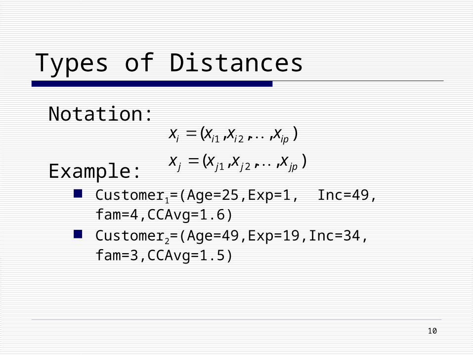
Types of Distances
Notation:
Example: Customer1=(Age=25,Exp=1, Inc=49,
fam=4,CCAvg=1.6) Customer2=(Age=49,Exp=19,Inc=34,
fam=3,CCAvg=1.5)
),,,(
),,,(
21
21
jpjjj
ipiii
xxxx
xxxx

11
Euclidean Distance
The Euclidean distance between the age of customer1 (25) and customer2 (49):
The Euclidean distance between the two on the 5-dimensions (Age, Exper, Income, Family, CCAvg):
2222
211 jpipjijiij xxxxxxd
[ (25-49)2 + (1-19)2 + (49-34)2 + (4-3)2 + (1.6-1.5)2]= =30.82
[ (25-49)2 ] = 24

which pair is closest ?
Income AgeCarry $31,779 36Sam $32,739 40Miranda $33,880 38
55%
27%
18%
1. Carry & Sam2. Sam & Miranda
3. Carry & Miranda
Carry & Sam: (31.779-32.739)2 + (36-40)2 = 960.00
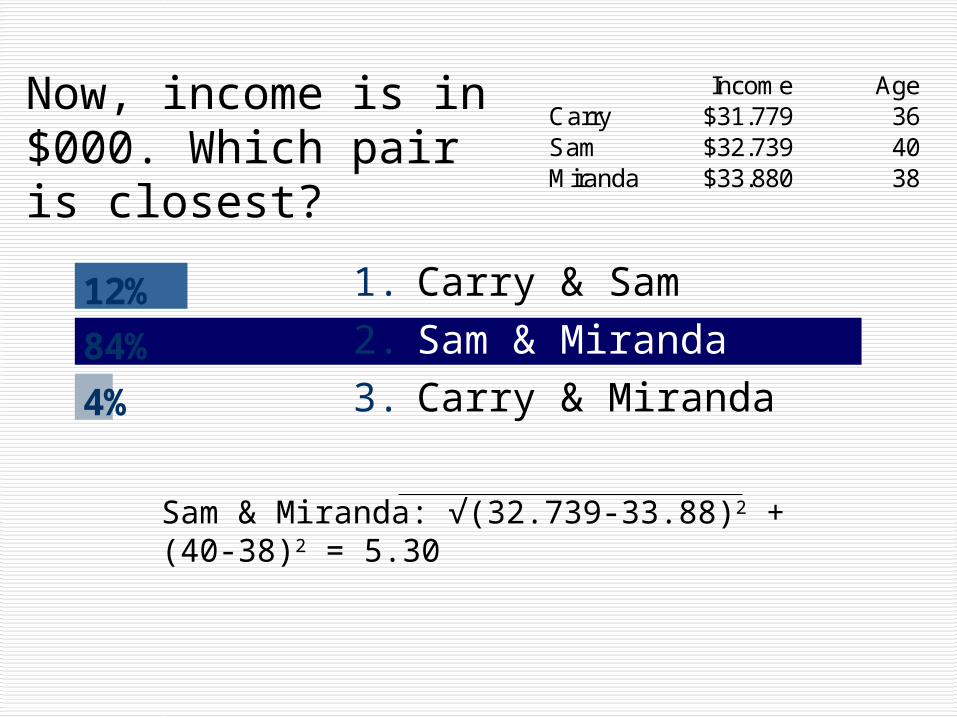
Now, income is in $000. Which pair is closest?
12%
84%
4%
1. Carry & Sam2. Sam & Miranda3. Carry & Miranda
Sam & Miranda: √(32.739-33.88)2 + (40-38)2 = 5.30
Income AgeCarry $31.779 36Sam $32.739 40Miranda $33.880 38
14
Why do we need to standardize the variables?
The distance measure is influenced by the units of the different variables, especially if there is a wide variation in units. Variables with “larger” units will influence the distances more than others.
The solution: standardize each variable before measuring distances!

15
Other distances Squared Euclidean distance Correlation-based distance: the correlation between
two vectors of (standardized) items/observations, rij, measures their similarity. We can define a distance measure as dij = 1- rij
2
Statistical distance (no need to standardize)
Manhattan distance (“city-block”)
Note: some software use “similarities” instead of “distances”.
jpipjijiij xxxxxxd 2211
Tjijiij xxSxxd 1 The only measure that accounts for covariance!

16
Distances for Binary Data
Are obtained from the 2x2 table of counts.
0 1
0 a b
1 c d
Married? Smoker? Manager?Carrie 1 1 1Sam 0 1 0Miranda 0 0 1
Carrie
Miranda 0 1
0
1
0
0 1
2

17
Choosing the number or neighbors (K)
Too small: under-smoothing Too large: over-smoothing Typically k<20 K should be odd (to avoid ties)
Solution: Use validation set to find “best” k

18
Output
1 0.00 4.15
2 1.30 4.45
3 2.47 4.10
4 2.10 3.80
5 3.40 4.50
Training Data scoring - Summary Report (for k=4)
0.5
Actual Class 1 0
1 243 43
0 20 2694
Class # Cases # Errors % Error
1 286 43 15.03
0 2714 20 0.74
Overall 3000 63 2.10
Validation Data scoring - Summary Report (for k=4)
0.5
Actual Class 1 0
1 134 60
0 16 1790
Class # Cases # Errors % Error
1 194 60 30.93
0 1806 16 0.89
Overall 2000 76 3.80
Error Report
Cut off Prob.Val. for Success (Updatable)
Classification Confusion Matrix
Predicted Class
Cut off Prob.Val. for Success (Updatable)
Classification Confusion Matrix
Predicted Class
Error Report
Validation error log for different k
Value of k% Error
Training% Error
Validation
1 0.00 4.15
2 1.30 4.45
3 2.47 4.10
4 2.10 3.80 <--- Best k
5 3.40 4.50
0.5
We’re using the validation data here to choose the best k
Lift chart (validation dataset)
0
50
100
150
200
250
0 1000 2000 3000
# cases
Cu
mu
lati
ve
CumulativePersonal Loanwhen sortedusing predictedvalues
CumulativePersonal Loanusing average

19
Advantages and Disadvantages of K nearest neighbors
The Good Very flexible, data-driven Simple With large amount of data, where predictor levels are
well represented, has good performance Can also be used for continuous y: instead of voting,
take average of neighbors (XLMiner: Prediction > K-NN)
The bad No insight about importance/role of each predictor Beware of over-fitting! Need a test set Can be computationally intensive for large k Need LOTS of data (exponential in #predictors)
20
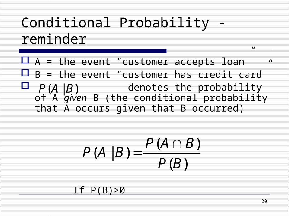
Conditional Probability - reminder
A = the event “customer accepts loan” B = the event “customer has credit card” denotes the probability of A given
B (the conditional probability that A occurs given that B occurred)
)(
)()|(
BP
BAPBAP
)|( BAP
If P(B)>0

21
Naïve Bayes Naive Bayes is one of the
most efficient and effective inductive learning algorithms for machine learning and data mining.
It calculates the probability of a point E to belong to a certain class Ci based on its attributes (x1, x2, …, xn) It assumes that the
attributes are conditional independent on the class Ci
C
x1 x2 xn….
22
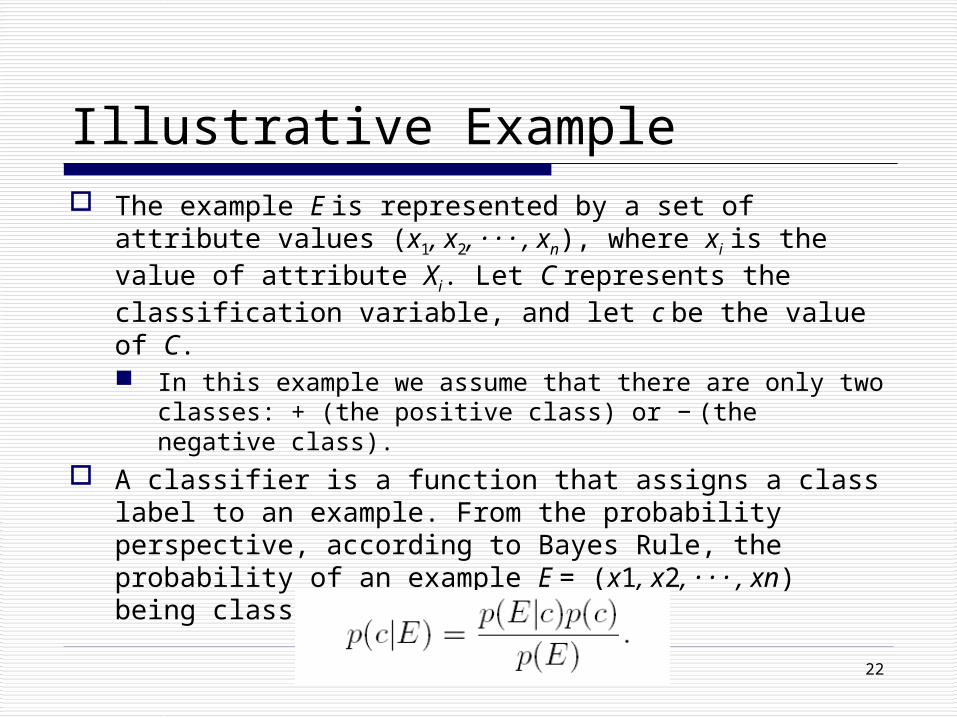
Illustrative Example The example E is represented by a set of attribute
values (x1, x2, · · · , xn), where xi is the value of attribute Xi. Let C represents the classification variable, and let c be the value of C. In this example we assume that there are only two
classes: + (the positive class) or − (the negative class).
A classifier is a function that assigns a class label to an example. From the probability perspective, according to Bayes Rule, the probability of an example E = (x1, x2, · · · , xn) being class c is

23
Naïve Bayes ClassifierE is classified as the class C = +if and only if:
where fb(E) is called a Bayesian classifier.Assume that all attributes are independent given the value of the class variable, that is:
The function fb(E) is called a naive Bayesian classifier,or simply naive Bayes (NB).
24
Augmented Naïve Bayes Naive Bayes is the simplest form of Bayesian network,
in which all attributes are independent given the value of the class variable.
This conditional independence assumption is rarely true in most real-world applications. A straightforward approach to overcome the
limitation of naive Bayes is to extend its structure to represent explicitly the dependencies among attributes.

25
Augmented Naïve BayesAn augmented naive Bayes (ANB), is an extended classifier, in which the class node directly points to all attribute nodes, and there exist links among attribute nodes. An ANB represents a joint probability distribution represented by:
where pa(xi) denotes an assignment to values of the parents of Xi. C
x1 x2 Xn-1…. xn
26
Why does this classifier work? The basic idea comes from
In a given dataset, two attributes may depend on each other, but the dependence may distribute evenly in each class.
Clearly, in this case, the conditional independence assumption is violated, but naive Bayes is still the optimal classifier.
What eventually affects the classification is the combination of dependencies among all attributes. If we just look at two attributes, there may exist strong
dependence between them that affects the classification.
When the dependencies among all attributes work together, however, they may cancel each other out and no longer affect the classification.
27
Why does this classifier work?
Definition 1:Given an example E, two classifiers f1 and f2 are said to be equal under zero-one loss on E, if f1(E) ≥ 0 if and only if f2(E) ≥ 0, denoted by f1(E) = f2(E) for every example E in the example space.
28
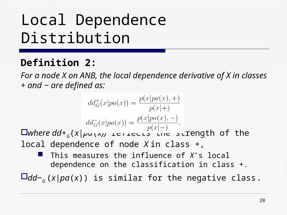
Local Dependence Distribution
Definition 2:For a node X on ANB, the local dependence derivative of X in classes + and − are defined as:
where dd+G(x|pa(x)) reflects the strength of the local dependence of node X in class +,
This measures the influence of X’s local dependence on the classification in class +.
dd−G (x|pa(x)) is similar for the negative class.
29
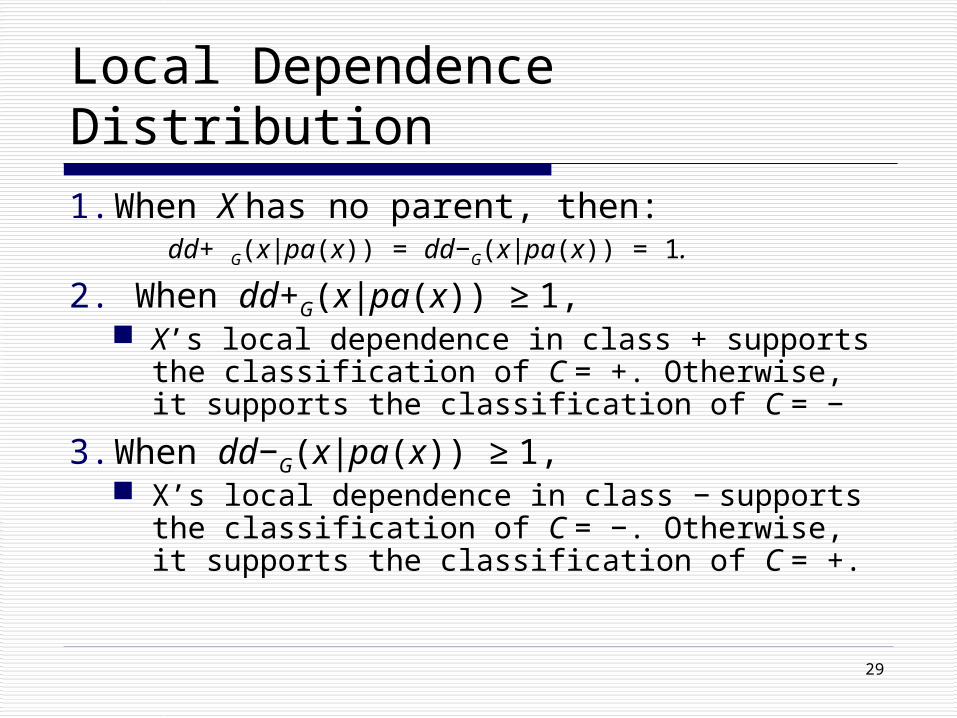
Local Dependence Distribution
1. When X has no parent, then: dd+ G(x|pa(x)) = dd−G(x|pa(x)) = 1.
2. When dd+G(x|pa(x)) ≥ 1, X’s local dependence in class + supports
the classification of C = +. Otherwise, it supports the classification of C = −
3. When dd−G(x|pa(x)) ≥ 1, X’s local dependence in class − supports
the classification of C = −. Otherwise, it supports the classification of C = +.

30
Local Dependence Distribution
When the local dependence derivatives in both classes support the different classifications, the local dependencies in the two classes cancel partially each other out,
The final classification that the local dependence supports, is the class with the greater local dependence derivative.
Another case is that the local dependence derivatives in the two classes support the same classification. Then, the local dependencies in the two classes work together to support the classification.
31
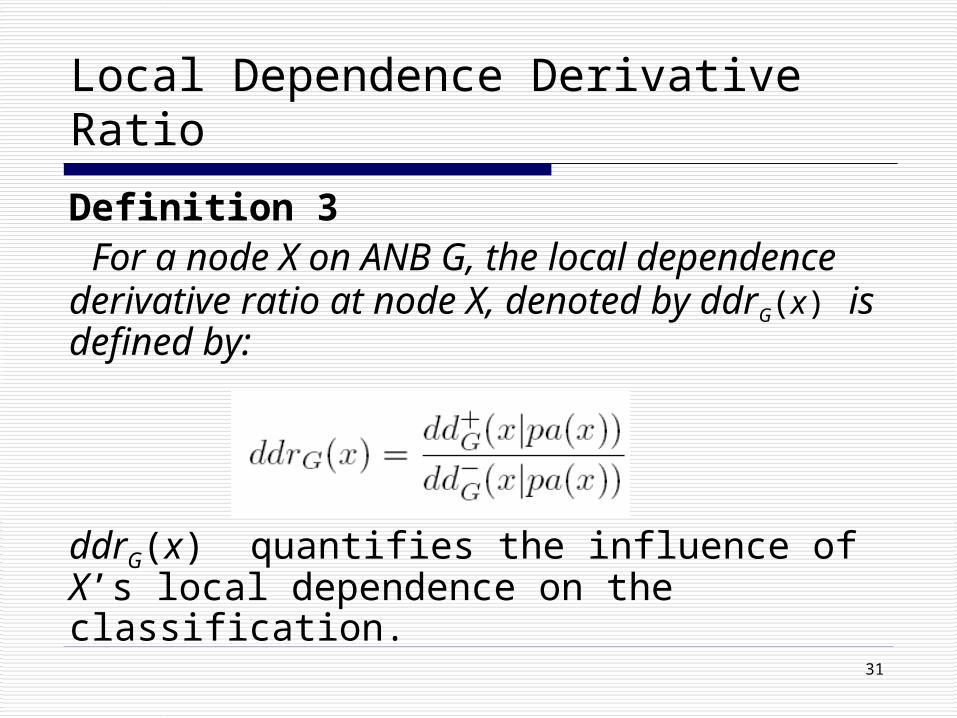
Local Dependence Derivative Ratio
Definition 3 For a node X on ANB G, the local dependence derivative ratio at node X, denoted by ddrG(x) is defined by:
ddrG(x) quantifies the influence of X’s local dependence on the classification.
32
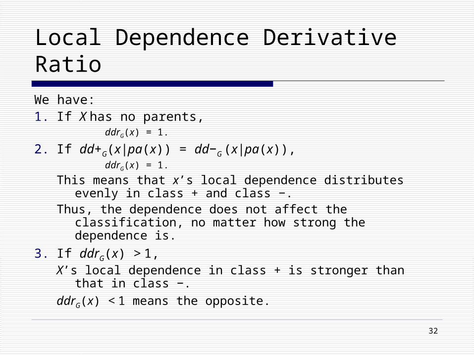
Local Dependence Derivative Ratio
We have:1. If X has no parents,
ddrG(x) = 1.
2. If dd+G(x|pa(x)) = dd−G (x|pa(x)), ddrG(x) = 1.
This means that x’s local dependence distributes evenly in class + and class −.
Thus, the dependence does not affect the classification, no matter how strong the dependence is.
3. If ddrG(x) > 1, X’s local dependence in class + is stronger than that in
class −. ddrG(x) < 1 means the opposite.
33
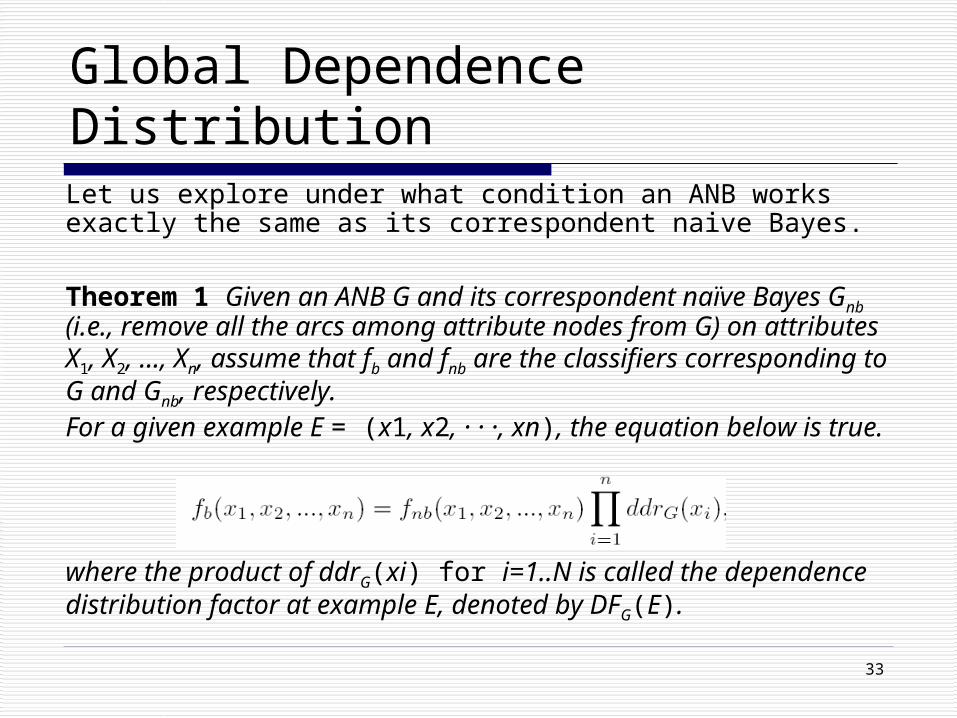
Global Dependence DistributionLet us explore under what condition an ANB works exactly the same as its correspondent naive Bayes.
Theorem 1 Given an ANB G and its correspondent naïve Bayes Gnb (i.e., remove all the arcs among attribute nodes from G) on attributes X1, X2, ..., Xn, assume that fb and fnb are the classifiers corresponding to G and Gnb, respectively.For a given example E = (x1, x2, · · ·, xn), the equation below is true.
where the product of ddrG(xi) for i=1..N is called the dependence distribution factor at example E, denoted by DFG(E).

34
Global Dependence Distribution
Proof:

35
Global Dependence Distribution
Theorem 2 Given an example E = (x1, x2, ..., xn), an ANB G is equal to its correspondent naive Bayes Gnb under zero-one loss if and only if when fb(E) ≥ 1, DFG(E) ≤ fb(E); or when fb(E) < 1, DFG(E) > fb(E).

36
Global Dependence DistributionApplying the theorem 2 we have the following
results:1. When DFG(E) = 1, the dependencies in ANB G
has no influence on the classification. The classification of G is exactly the same as that of
its correspondent naïve Bayes Gnb. There exist three cases for DFG(E) = 1.
no dependence exists among attributes. for each attribute X on G, ddrG(x) = 1; that is, the
local distribution of each node distributes evenly in both classes.
the influence that some local dependencies support classifying E into C = +is canceled out by the influence that other local dependences support classifying E into C = −.
37
Global Dependence Distribution
2. fb(E) = fnb(E) does not require that DFG(E) = 1. The precise condition is given by Theorem 2. That explains why naive Bayes still produces accurate classification even in the datasets with strong dependencies among attributes (Domingos & Pazzani 1997).
3. The dependencies in an ANB flip (change) the classification of its correspondent naive Bayes, only if the condition given by Theorem 2 is no longer true.
38
Conditions of the optimality of the Naïve Bayes
Naive Bayes classifier is optimal if the dependencies among attributes cancel each other out.
The classifier is still optimal even though the dependencies do exist
39
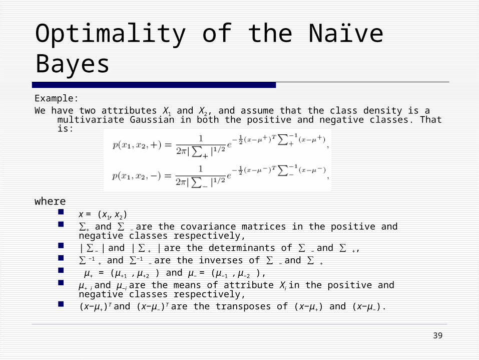
Optimality of the Naïve BayesExample:We have two attributes X1 and X2, and assume that the class density is a
multivariate Gaussian in both the positive and negative classes. That is:
where x = (x1, x2) ∑+ and ∑ − are the covariance matrices in the positive and negative
classes respectively, | ∑ − | and | ∑ + | are the determinants of ∑ − and ∑ +, ∑ −1
+ and ∑−1 − are the inverses of ∑ − and ∑ +
μ+ = (μ+1 , μ+2 ) and μ− = (μ−1 , μ−2 ), μ+ i and μ−i are the means of attribute Xi in the positive and negative
classes respectively, (x−μ+)T and (x−μ−)T are the transposes of (x−μ+) and (x−μ−).

40
Optimality of the Naïve BayesWe assume:The two classes have a common covariance matrix ∑+ = ∑− = ∑ ,
X1 and X2 have the same variance σ in both classes.
Then, when applying a logarithm to the Bayesian classifier, defined previously, we obtain the following fb classifier

41
Optimality of the Naïve Bayes Then, because of the conditional independence
assumption, we have the correspondent naive Bayesian classifier fnb
Assume that
X1 and X2 are independent if σ12 = 0. If σ ≠ σ12, we have:

42
Optimality of the Naïve Bayes
An example E is classified into the positive class by fb, if and only if fb ≥ 0. fnb is similar.
When fb or fnb is divided by a non-zero positive constant, the resulting classifier is the same as fb or fnb. Then

43
Optimality of the Naïve Bayes
where a = − (1/σ2)(μ+ + μ−)Σ−1(μ+ − μ−), is a constant independent of x.
For any x1 and x2, Naive Bayes has the same classification as that of the underlying classifier if:

44
Optimality of the Naïve Bayes
This is:
1

45
Optimality of the Naïve Bayes
Assuming that:
We can simplify the equation to:
where
1

46
Optimality of the Naïve Bayes
The shaded area of the figure shows the region in which the Naïve Bayes Classifier is optimal

47
Example with 2 predictors: CC, Online
P(accept =1 | CC=1, online=1) =
)0()0|1,1()1()1|1,1(
)1()1|1,1(
acceptPacceptOnlineCCPacceptPacceptOnlineCCP
acceptPacceptOnlineCCP50/286
Count of Personal Loan OnlineCreditCard Personal Loan 0 1 Grand Total
0 0 769 1163 19321 71 129 200
0 Total 840 1292 21321 0 321 461 782
1 36 50 861 Total 357 511 868Grand Total 1197 1803 3000
286/3000

P(CC=1, Online=1 | accept=0) is approx
20%
20%
20%
20%
20% 1. 50/2862. 1-50/2863. 461/30004. 461/(3000-286)5. 129/(3000-286)

49
Example with 2 predictors: CC, Online
P(accept =1 | CC=1, online=1) =
)0()0|1,1()1()1|1,1(
)1()1|1,1(
acceptPacceptOnlineCCPacceptPacceptOnlineCCP
acceptPacceptOnlineCCP
0978.0
30002714
2714461
3000286
28650
3000286
28650

50
The practical difficulty
We need to have ALL the combinations of predictor categories CC=1,Online=1 CC=1, Online=0 CC=0, Online=1 CC=0, Online=0
With many predictors, this is pretty unlikely

51
Example with (only) 3 predictors: CC, Online, CD account
Count of Personal Loan CD Account Online0 0 Total 1 1 Total Grand Total
CreditCard Personal Loan 0 1 0 10 0 769 1152 1921 11 11 1932
1 69 100 169 2 29 31 2000 Total 838 1252 2090 2 40 42 2132
1 0 318 363 681 3 98 101 7821 30 30 6 50 56 86
1 Total 348 363 711 9 148 157 868Grand Total 1186 1615 2801 11 188 199 3000
CD account=0, Online=1, CreditCard=1

52
A practical solution: From Bayes to Naïve Bayes
Substitute P(CC=1,Online=1 | accept) with P(CC=1 | accept) x P(Online=1 | accept)
This means that we are assuming independence between CC and Online!
If the dependence is not extreme, it will work reasonably well

53
Example with 2 predictors: CC, Online
P(accept =1 | CC=1, online=1) =
)0()0|1,1()1()1|1,1((
)1()1|1,1(
acceptPacceptOnlineCCPacceptPacceptOnlineCCPP
acceptPacceptOnlineCCP
Count of Personal Loan OnlineCreditCard Personal Loan 0 1 Grand Total
0 0 769 1163 19321 71 129 200
0 Total 840 1292 21321 0 321 461 782
1 36 50 861 Total 357 511 868Grand Total 1197 1803 3000
)1|1()1|1( acceptOnlinePacceptCCP
)0|1()0|1( acceptOnlinePacceptCCP

54
Naïve Bayes for CC, Online: P(accept =1 | CC=1, online=1) =
)0()0|1,1()1()1|1,1((
)1()1|1,1(
acceptPacceptOnlineCCPacceptPacceptOnlineCCPP
acceptPacceptOnlineCCP
102.0
30002714
27141642
2714782
3000286
286179
28686
3000286
286179
28686
)1|1()1|1( acceptOnlinePacceptCCP
)0|1()0|1( acceptOnlinePacceptCCP
Count of Personal Loan OnlinePersonal Loan 0 1 Grand Total
0 1090 1624 27141 107 179 286
Grand Total 1197 1803 3000
Count of Personal Loan CreditCardPersonal Loan 0 1 Grand Total
0 1932 782 27141 200 86 286
Grand Total 2132 868 3000

55
Naïve Bayes in XLMiner
Classification> Naïve Bayes
Prior class probabilities
Prob.
0.095333333
0.904666667
Value Prob Value Prob
0 0.374125874 0 0.401621223
1 0.625874126 1 0.598378777
0 0.699300699 0 0.711864407
1 0.300699301 1 0.288135593
Online
CreditCard
Classes-->
1 0Input Variables
1
0
<-- Success Class
Conditional probabilities
According to relative occurrences in training data
Class
P(CC=1| accept=1) = 86/286

56
Naïve Bayes in XLMiner
Scoring the validation data
XLMiner : Naive Bayes - Classification of Validation Data
0.5
Row Id.Predicted
ClassActual Class
Prob. for 1 (success)
Online CreditCard
2 0 0 0.08795125 0 0
3 0 0 0.08795125 0 0
7 0 0 0.097697987 1 0
8 0 0 0.092925663 0 1
11 0 0 0.08795125 0 0
13 0 0 0.08795125 0 0
14 0 0 0.097697987 1 0
15 0 0 0.08795125 0 0
16 0 0 0.10316131 1 1
Cut off Prob.Val. for Success (Updatable) ( Updating the value here will NOT update value in summary report )
Data range['UniversalBank KNN NBayes.xls']'Data_Partition1'!$C$3019:$O$5018

57
Advantages and Disadvantages The good
Simple Can handle large amount of predictors High performance accuracy, when the goal is ranking Pretty robust to independence assumption!
The bad Requires large amounts of data Need to categorize continuous predictors Predictors with “rare” categories -> zero prob (if this
category is important, this is a problem) Gives biased probability of class membership No insight about importance/role of each predictor