BrianG.Keating,1 ChristopherW.O’Dell,...

AN INSTRUMENT FOR INVESTIGATING THE LARGE ANGULAR SCALE POLARIZATION OF THECOSMIC MICROWAVE BACKGROUND

Brian G. Keating,1ChristopherW. O’Dell, Joshua O. Gundersen,

2Lucio Piccirillo,

3Nate C. Stebor,

4

and Peter T. Timbie

Department of Physics, 2531 Sterling Hall, University ofWisconsin—Madison,Madison,WI 53706Received 2001 November 14; accepted 2002 August 30

ABSTRACT

We describe the design and performance of a microwave polarimeter used to make precisionmeasurementsof polarized astrophysical radiation in three microwave frequency bands spanning 26–36 GHz. Theinstrument uses cooled HEMT amplifiers in a correlation polarimeter configuration to achieve high sensitiv-ity and long-term stability. The instrument demonstrates long-term stability and has produced the mostrestrictive upper limits to date on the large angular scale polarization of the 2.7 K cosmic microwave back-ground radiation.

Subject headings: cosmic microwave background — cosmology: observations —instrumentation: polarimeters — radio continuum: general

1. INTRODUCTION

Observations of the cosmic microwave background(CMB) are some of the most powerful tools in cosmology.The CMB has the promise to address the most fundamentalcosmological questions: the geometry and age of theuniverse, the matter content of the universe, the ionizationhistory, and the spectrum of primordial perturbations. TheCMB is specified by three characteristics: its spectrum, thespatial distribution of its total intensity, and the spatial dis-tribution of its polarization. All three properties depend onthe fundamental cosmological parameters. Several instru-ments have produced precision measurements of its spec-trum and anisotropy at large, medium, and small angularscales (see, e.g., Wang, Tegmark, & Zaldarriaga 2001 andreferences therein).

Similar to the CMB anisotropy power spectrum, thepolarization power spectrum encodes information on allangular scales. Large angular scales (>1�) correspond toregions on the last scattering surface that were larger thanthe causal horizon at that time. In the absence of reioniza-tion, polarization on these scales was affected only by thelongest wavelength modes of the primordial power spec-trum. Reionization is expected to produce a new polarizedpeak in the power spectrum near ‘d20, where the precisepeak location depends on the redshift at which the universe(Zaldarriaga 1998; Keating et al. 1998) became reionized.

The large-scale region of the anisotropy power spectrumwas measured by the COBE DMR, and this established thenormalization for models of large-scale structure formation.The effect of reionization on the anisotropy power spectrumis to damp all angular scales by a factor of e�2� , where � isthe optical depth to the reionization epoch. This effect is

degenerate with several other cosmological parameters(Zaldarriaga 1997), and nonzero � cannot be unambigu-ously detected, at any scale, from the anisotropy powerspectrum alone. Similarly, the effect of gravitational waveson the anisotropy power spectrum is also degenerate withother cosmological parameters (Zaldarriaga, Spergel, &Seljak 1997). Detection of CMB polarization at scales >1�

has the potential to detect reionization and primordialgravitational waves.

Although the polarization signal at large angular scales isexpected to be weaker than at small scales, the design of alarge angular scale experiment is simpler and more compactthan an experiment probing small scales. A large angularscale experiment with no external beam forming optics (i.e.,no primary mirror), exhibits minimal spurious polarizationand reduces susceptibility to numerous sources of system-atic error. In this paper we describe our approach to meas-uring the large-scale polarization of the CMB: PolarizationObservations of Large Angular Regions (POLAR).

POLAR’s design builds on techniques developed in pre-vious searches for CMB polarization (Nanos 1979; Lubin &Smoot 1981; Wollack et al. 1997) and is driven by the sizeand angular scale of the anticipated CMB signals, spectralremoval of foreground sources, optimization of the observ-ing scheme, long-term stability, and immunity to potentialsystematic effects. POLAR is a wide bandwidth (�8 GHz)correlation polarimeter dedicated to measurements of theCMB. POLAR measures polarization in the Ka band,between 26 and 36 GHz, using cooled High Electron Mobi-lity Transistor (HEMT) amplifiers. This band is multiplexedinto three sub-bands to allow for discrimination againstforeground sources. The radiometer executes a zenith driftscan with a 7� FWHM beam produced by a corrugated feedhorn antenna. In the Spring of 2000 POLAR observed a’7� wide region from R:A: ¼ 112� to 275� at declination43� for 45 days from the University of Wisconsin—Madi-son’s Pine Bluff Observatory in Pine Bluff, Wisconsin (Lati-tude +43�010, Longitude +89�450). In a single night of dataPOLAR achieved a sensitivity level of�50 lK to the Stokesparameters Q and U in each beam-sized pixel. For the 2000season POLAR set upper limits on the amplitude of the cos-mological E-mode and B-mode (Zaldarriaga & Seljak 1997;

1 Current Address: Division of Physics, Math, and Astronomy,California Institute of Technology, Pasadena, CA 91125;[email protected].

2 Department of Physics, University ofMiami, Coral Gables, FL 33146.3 Department of Physics and Astronomy, University of Wales—Cardiff

CF24 3YB,Wales, UK.4 Department of Physics, University of California at Santa Barbara,

Santa Barbara, CA 93106.

The Astrophysical Journal Supplement Series, 144:1–20, 2003 January

# 2003. The American Astronomical Society. All rights reserved. Printed in U.S.A.

1

Kamionkowski, Kosowsky, & Stebbins 1997) power spectraof TE , TB < 10 lK at 95% confidence (Keating et al. 2001).

In this paper we describe the design and performance ofPOLAR. In x 2 we outline the fundamentals of the correla-tion polarimeter. Section 3 presents detailed instrumentdesign specifications and performance. Section 4 describesour calibration technique, and x 5 addresses potential sys-tematic effects and radiometric offset characterization.Finally, x 6 summarizes the meteorological conditionsencountered during the observation run as well as our dataselection criteria.

2. CORRELATION POLARIMETER

The correlation polarimeter is based on a correlationradiometer (Fujimoto 1964; Rohlfs 1996), which sharesmany technological features with an interferometer(Thompson et al. 1998). The development of the correlationradiometer preceded the discovery of the CMB in 1965; see,for example, Fujimoto (1964). Several early CMB experi-ments used correlation radiometers for anisotropy measure-ments (Cheng et al. 1979), spectral measurements (Johnson& Wilkinson 1987), and the first application of a dedicatedinterferometer to CMB research (Timbie & Wilkinson1990).

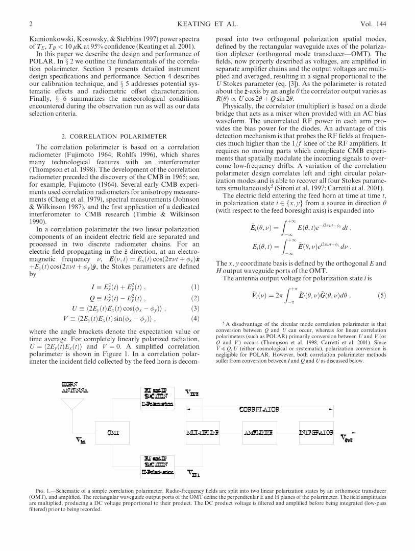
In a correlation polarimeter the two linear polarizationcomponents of an incident electric field are separated andprocessed in two discrete radiometer chains. For anelectric field propagating in the zz direction, at an electro-magnetic frequency �, Eð�; tÞ ¼ ExðtÞ cosð2��tþ �xÞxxþEyðtÞ cosð2��tþ �yÞyy, the Stokes parameters are definedby

I � E2xðtÞ þ E2

yðtÞ ; ð1ÞQ � E2

xðtÞ � E2yðtÞ ; ð2Þ

U � h2EyðtÞExðtÞ cosð�x � �yÞi ; ð3ÞV � h2EyðtÞExðtÞ sinð�x � �yÞi ; ð4Þ

where the angle brackets denote the expectation value ortime average. For completely linearly polarized radiation,U ¼ h2EyðtÞExðtÞi and V ¼ 0. A simplified correlationpolarimeter is shown in Figure 1. In a correlation polar-imeter the incident field collected by the feed horn is decom-

posed into two orthogonal polarization spatial modes,defined by the rectangular waveguide axes of the polariza-tion diplexer (orthogonal mode transducer—OMT). Thefields, now properly described as voltages, are amplified inseparate amplifier chains and the output voltages are multi-plied and averaged, resulting in a signal proportional to theU Stokes parameter (eq. [3]). As the polarimeter is rotatedabout the zz-axis by an angle h the correlator output varies asRð�Þ / U cos 2�þQ sin 2�.

Physically, the correlator (multiplier) is based on a diodebridge that acts as a mixer when provided with an AC biaswaveform. The uncorrelated RF power in each arm pro-vides the bias power for the diodes. An advantage of thisdetection mechanism is that probes the RF fields at frequen-cies much higher than the 1=f knee of the RF amplifiers. Itrequires no moving parts which complicate CMB experi-ments that spatially modulate the incoming signals to over-come low-frequency drifts. A variation of the correlationpolarimeter design correlates left and right circular polar-ization modes and is able to recover all four Stokes parame-ters simultaneously5 (Sironi et al. 1997; Carretti et al. 2001).

The electric field entering the feed horn at time at time t,in polarization state i 2 fx; yg from a source in direction h(with respect to the feed boresight axis) is expanded into

~EEið�; �Þ ¼Z þ1

�1Eð�; tÞe�i2��t��i dt ;

Eið�; tÞ ¼Z þ1

�1~EEð�; �Þei2��tþ�i d� :

The x, y coordinate basis is defined by the orthogonal E andH output waveguide ports of the OMT.

The antenna output voltage for polarization state i is

~VVið�Þ ¼ 2�

Z þ�

��

~EEið�; �Þ~GGð�; �Þd� ; ð5Þ

Fig. 1.—Schematic of a simple correlation polarimeter. Radio-frequency fields are split into two linear polarization states by an orthomode transducer(OMT), and amplified. The rectangular waveguide output ports of the OMT define the perpendicular E and H planes of the polarimeter. The field amplitudesare multiplied, producing a DC voltage proportional to their product. The DC product voltage is filtered and amplified before being integrated (low-passfiltered) prior to being recorded.

5 A disadvantage of the circular mode correlation polarimeter is thatconversion between Q and U can occur, whereas for linear correlationpolarimeters (such as POLAR) primarily conversion between U and V (orQ and V ) occurs (Thompson et al. 1998; Carretti et al. 2001). SinceV5Q;U (either cosmological or systematic), polarization conversion isnegligible for POLAR. However, both correlation polarimeter methodssuffer from conversion between I andQ andU as discussed below.

2 KEATING ET AL. Vol. 144

where ~GGð�; �Þ is the horn’s (axisymmetric) voltage responsefunction. The output voltage for each polarization, afteramplification with total radiometer voltage transfer func-tion ~HHð�Þ, is V 0

i ð�Þ ¼ ~HHð�Þ ~VVið�Þ. The correlator producesthe complex correlation function, at time lag � , of the twovoltages:

Rð�Þ ¼ limT!1

4�2

2T

Z þT

�T

VxðtÞV�y ðt� �Þdt

¼ limT!1

4�2

2T

Z þT

�T

dt

Z þ1

�1d�x

Z þ1

�1d�y

Z �

0

d�x

Z �

0

d�y

� ~EExð�; �xÞ~EE�y ð�0; �yÞ ~HHxð�xÞ ~HH�y ð�yÞ~GGxð�x; �xÞ

� ~GG�y ð�y; �yÞeið2��xtþ�xÞe�ið2��yðt��Þþ�yÞ : ð6Þ

Remembering thatRþ1�1 e2�itð�x��yÞ dt ¼ �ð�x � �yÞ, we

obtain

Rð�Þ ¼ 4�2

Z þT

�T

Z �

0

Z �

0

d� d�x d�y

� ~��ð�; �x; �yÞ~BBð�; �Þ ~HHxð�Þ ~HH�y ð�Þeið2��þD�Þ ; ð7Þ

where

~��ð�; �x; �yÞ ¼ limT!1

1

2T½~EExð�; �Þ~EE�y ð�0; �Þ� ð8Þ

is the source coherence function, D� ¼ �x � �y, and

~BBð�; �x; �yÞ ¼ ~GGxð�x; �Þ~GG�y ð�y; �Þ :

In practice, it is not necessary to enforce T ! 1, aslong as T41=�. If, as is the case for POLAR,~GGxð�x; �Þ ’ ~GGyð�y; �Þ � ~GGð�; �Þ, then Bð�; �Þ ¼ j~GGð�; �Þj2 isthe power response function of the horn, or beam pattern.For a thermal source, such as the CMB,~��ð�; �; �0Þ ¼ ~��ð�; �Þ�ð�� 0Þ. For POLAR ~HHxð�Þ ’ ~HHyð�Þ� ~HHð�Þ, and only the real part of the complex correlationfunction is measured with zero lag. Thus, POLAR’s outputcan be expressed as

Ro ¼ 4�2

Z þ1

�1d�

Z þ�

0

d� ~��ð�; �Þ~BBð�; �Þj ~HHð�Þj2 cosðD��Þ ;

ð9Þ

where the subscript � on D� incorporates a (potentially) fre-quency dependent phase shift between the two arms of theradiometer; see x 5.3. The properties of the source coherencefunction, the transfer functions, and the beam responsecompletely determine the output voltage. Equation (9) willbe useful in x 4, where POLAR’s response to completely cor-related, polarized signals produced by calibration sources iscomputed.

2.1. MinimumDetectable Signal

The sensitivity of the correlation polarimeter depends onboth the system noise temperature and the RF bandwidthof the system. Since there are two RF amplifier chains, thesystem temperature is their geometric mean: Tsys ¼TEsysTH

sys

� �1=2, and the minimum detectable signal in an

integration time � is

DT ¼

ffiffiffiffiffiffiffiffiffiffiffiffiffiffiffiffiffiffiffiffiffiffiffiffiffiffiffiffiffiffiffiffiffiffiffi2TE

sysTHsys

D�RF� cos2hD�i�

s; ð10Þ

where D�RF is the RF bandwidth, and E and H refer to theorthogonal polarization states separated by the OMT(Thompson et al. 1998). Here we define hD�i� as the band-averaged [

R10 D�ð�Þd�=

R10 D�2ð�Þd�] differential phase

shift between the two arms prior to correlation. Dependingon the physical nature of the differential phase shift (e.g.,differential guide length, dielectric or microstrip dispersion,etc.) the phase shift may be calculable and/or separablefrom other sources of bandwidth degradation. In POLAR,all passive waveguide components are matched in length,and adjustable coaxial phase shifters prior to correlation areemployed to minimize the contribution of path length phasedifferences. Equation (10) is valid only when there are noRF gain or offset fluctuations. The effects of radiometer off-set, stability, and other nonidealities are discussed in x 5.

3. THE POLAR RADIOMETER

POLAR’s radiometer (Fig. 2) is comprised of three sec-tions: (1) cold receiver components: optics, OMT, isolators,HEMT amplifiers, (2) room-temperature receiver compo-nents: warm RF amplifiers, heterodyne stage, warm IFamplifiers, band-defining filters, correlators, and (3) postde-tection components: preamplifiers, low-frequency process-ing, and data acquisition. In this section the details of theexperimental design are presented.

3.1. Cryogenics

The Dewar (Fig. 3) was custom fabricated6 to house acryocooler coldhead and is large enough to accommodatepossible upgrades including additional feed horns in thenominal 20 K (second stage) working volume. The firststage is used to cool a radiation shield, which is maintainedat a nominal temperature of�80 K.

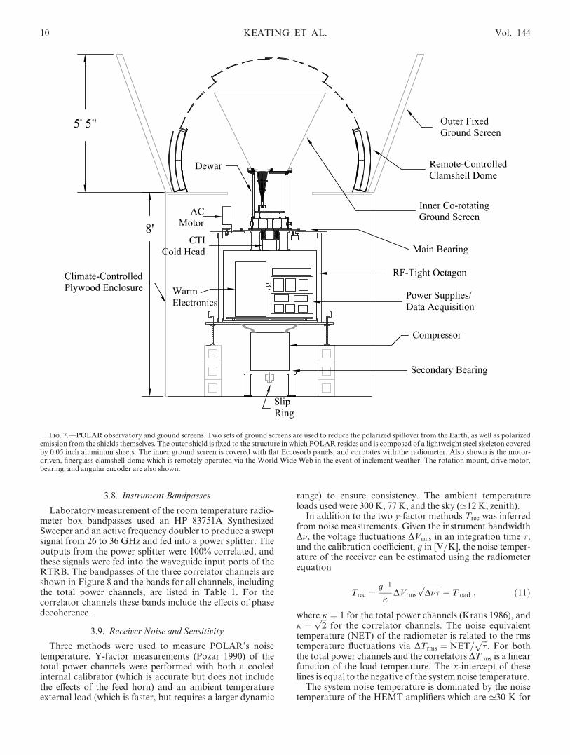
Following pump-down to �1� 10�4 torr, the pump isdetached and the cryocooler’s compressor (CTI 8500 AirCooled) is activated. In the field it was found that the ulti-mate cold stage temperatures are correlated with the ambi-ent temperature of the shelter in which POLAR resides. Thecompressor is air-cooled; water cooling was not possibledue to the receiver’s continuous rotation. The air coolingcauses the compressor’s compression ratio to be a functionof ambient temperature, which modifies its cooling effi-ciency. Maintaining the temperature stability of the com-pressor is accomplished, to first order, by a commercialair-conditioner during the summer months which countersthe �2 kW heat output from the compressor. During thewinter, the heat output by the compressor kept the enclosedPOLAR shelter at a nearly constant temperature. The com-pressor is mechanically isolated from the radiometer by useof a separate rotation bearing coupled loosely to the motor-driven main bearing by copper braid (see Fig. 7). The com-pressor is further isolated on its bearing by use of rubberpadding on all support structures.

The cold radiometer components are mounted on the 20K stage, located inside the 80 K stage radiation shield. Bothwaveguide outputs from the HEMTs connect to vacuum-tight WR-28 stainless steel waveguide feedthroughs7 on the300 K Dewar wall. The feedthroughs are mounted on a sin-gle flange, which also serves as a feedthrough for the HEMT

6 Precision Cryogenic Systems: Indianapolis, IN.7 Aerowave Corp.:Medford,MA.

No. 1, 2003 CMB LARGE ANGULAR SCALE POLARIZATION 3

Fig. 2.—Schematic of the POLARKa-band correlation polarimeter

bias wiring and the temperature diode readout wiring. Thefinal major port in the Dewar is the main vacuum opticalwindow. This port is located �3 inches radially off the rota-tion axis of the cryostat to allow for additional feed horns athigher frequency.

3.2. Optics

POLAR’s RF optical system is composed of a single cor-rugated feed horn. Due to the absence of supplementalbeam-forming reflectors, cross-polarization of the instru-ment is near the minimum possible level for a millimeterwave receiver. POLAR’s feed horn design is based on theprocedure outlined in Zhang et al. (1993) and is similar tothe Ka-band feed horn employed by the COBE DMRexperiment (Janssen et al. 1979). The horn exhibits sym-

metry between its E and H planes and produces adiffraction-limited power response with a ’7� full width athalf-maximum (FWHM) across the band.

The beam pattern for the POLAR feed was computedusing an 11 term Gauss-Laguerre model (Clarricoats &Olver 1984) to predict the far-field beam pattern out to�20�. A comparison of the measured and modeled beams isillustrated in Figure 4. The simple Gauss-Laguerre modelbreaks down at low-power levels, which translates to the faroff-axis response of the horn at � � 20�. In the absence of areliable model for the far off-axis behavior of our feed, wemeasured the beam response for a variety of frequencies, forboth polarizations, as well as the cross-polarizationresponse (see Fig. 5).

The final component of the feed horn is the mode con-verter, which is a separate electroformed element at the

Fig. 3.—POLAR Dewar and Ka-band cold receiver components. The horn is located off of the symmetry axis of the Dewar in order to allow for futurereceivers to perform simultaneous observations. TheHEMToutputs travel via stainless steel waveguides to a flange on the Dewar bottom.

CMB LARGE ANGULAR SCALE POLARIZATION 5

throat of the horn. The mode converter combines the TE�11

and TM�11 circular waveguide modes to create the hybrid

HE�11 corrugated waveguide mode (Clarricoats & Olver

1984; Zhang et al. 1993). Following the throat in the opticalpath, there is an electroformed transition from the throat’scircular output waveguide to the square-input waveguide ofthe OMT. This device was designed by matching the cutoffwavelengths of the TE&

10 and the HE�11 modes.

3.3. Orthomode Transducer (OMT)

The OMT (variously referred to as a: polarizationdiplexer, dual-mode transducer, orthomode tee, and ortho-mode junction) is a waveguide device used to separate thetwo orthogonal linear polarization states. POLAR’s OMT 8

Fig. 4.—Gauss-Laguerre and Gaussian beam models compared to measured beam patterns. The diamonds (26 GHz), triangles (29 GHz), and squares (36GHz) are the measured beam patterns in the E-plane. The solid lines represent the corresponding Gauss-Laguerre approximations, and the dashed lines arethe best-fit Gaussians to the main beam of the measured data.

Fig. 5.—Beam maps of the feed horn measured at 29 GHz are shown. The solid line is the copolar E-plane power response pattern, the dashed line is thecopolar H-plane pattern, the dotted line is the E-plane cross-polarization response, and the dot-dashed line is the cross-polarization measured at 45� to theE-plane.

8 AtlanticMicrowave: Bolton,MA,Model OM 2800.


is a three-port device with a square input port, and tworectangular output ports containing the orthogonal polar-ization signals.

The OMT’s entrance port is a Ka-band square guide thatsimultaneously supports both TE&

01 and TE&10 modes. After

the modes are separated by the OMT they are further iso-lated using cryogenic Ka-band isolators.9 The isolators pre-vent coupling of the polarization states from reflection byhigh-VSWR components (such as the HEMT amplifiers).After leaving the OMT the fields in each of the two polariza-tion states are amplified, downconverted, and filtered sepa-rately until correlation. POLAR’s OMT can be describedby a 4� 4 scattering matrix, Sij. Element 1 in the S-matrixrefers to the input port with E-plane polarization, while 2, 3,and 4 refer to input H-plane, output E-plane, and output H-plane, respectively. On-diagonal elements of Sij such as S11

and S22 define the return loss for input E-plane and H-planepolarization states. The terms S13 and S24 determine thecopolar transmission/forward loss and are not necessarilyequal. Differential loss (e.g., S13 6¼ S24 will lead to instru-mental polarization and/or depolarization. The off-diagonal terms S34 ¼ S43 characterize the output polariza-tion isolation, and the terms S14 and S23 define the OMT’scross-polarization. Plots of the OMT performance are dis-played in Figure 12. As described in x 5, an offset in the out-put of the correlation polarimeter can be caused by eithernonzero cross polarization or isolation.

3.4. Signal Processing

POLAR’s High Electron Mobility Transistor (HEMT)amplifiers (Pospieszalski 1992) provide a gain of �30 dB.POLAR’s amplifiers utilize InP based devices for the firststage (which have lower noise-temperatures than GaAsdevices) at the expense of slightly increased 1=f noise. How-ever, the low-frequency spectral properties of these ampli-fiers are largely irrelevant for correlation radiometers sincethe multiplication is performed at several-GHz, i.e., wellabove the few-Hz knee of the HEMTs. POLAR’s twoamplifiers have noise temperatures of ’30 K. Figure 11shows the low-frequency power spectra of the total powerradiometer channels (dominated by the HEMTs) comparedto the spectra of the correlator channels.

3.4.1. Room Temperature Radiometer Box (RTRB)

After amplification by HEMTs, the RF signals are routedto straight 6 inch long stainless steel waveguides which pro-vide a thermal break from the 20 K HEMTs to the 300 KDewar walls. The stainless guides are bolted to the vacuum-tight WR-28 waveguide feedthroughs. Outside the Dewar,straight sections of rhodium plated, brazed-copper wave-guides are used to compensate for the path-lengthdifferences between the two polarizations incurred by thebends. Finally, the waveguides enter the room temperatureradiometer box (RTRB), where the signals are convertedfrom waveguide to coax to match the inputs of the Ka-bandwarm HEMT amplifiers.10 The noise temperatures of thesedevices are TN ’ 230 K.

3.4.2. Superheterodyne Components

Following the second-stage of amplification, the signalsare down-converted in frequency from 26–36 GHz to 2–12GHz by a 38 GHz local oscillator11 (LO) and superhetero-dyne mixers.12 The IF spectrum is a (scaled) replica of theinput RF band, with a nearly identical bandwidth. Twostages of IF (2–12 GHz) amplification are used13 to providethe appropriate bias power level into the multipliers. Thegain of the IF amplifiers fall steeply above a frequency off3 dB ’ 12 GHz. Since each multiplier requires �5 mW ofbias power, the IF signal must be amplified by �60 dB.After mixing and IF amplification the signals are dividedinto two paths. One path, referred to as the ‘‘ total powerdetector ’’ channels (TP-E and TP-H) is detected bySchottky diodes.14 ‘‘ E ’’ and ‘‘H ’’ refer to the OMT port inwhich the respective total power signal originates. The otherpost-IF gain path is sent into a frequency triplexer.15 Thefunction of the triplexers is threefold. First they producethree (ideally) independent bands with which are used toinvestigate the spectral behavior of the data. Second, thesedevices allow us to flatten the gain of the system across thewide RF-bandwidth provided by the HEMTs. Finally, thedifferential phase between the two arms can be made flatteracross the sub-bands than across the full RF band. Prior tocorrelation the gain and phase of each sub-band arematched with fixed attenuators and phase shifters.16

3.4.3. Correlators

POLAR’s correlator is a Schottky-diode mixer.17 Amixer-based correlator is composed of a double balancedmixer, a phase modulating element, and lock-in detection.The primary difference between a multiplier and a conven-tional mixer is that the IF bandwidth of the multiplier ismade intentionally narrow to suppress frequency compo-nents greater than �100 MHz, and the output of the multi-plier can support DC.

The RF band passes of the multipliers are from 1 to 12GHz, and the IF bandpasses are from 0 to 100MHz. The IFoutput port is not transformer-coupled, and propagates theDC signal proportional to the correlation between signals inthe x and y polarization states. Phase modulation andphase-sensitive detection (PSD) is accomplished by an elec-tronic 0�–180� phase shifter,18 and a synchronous demodu-lator19 and integrator. The phase of the LO is switchedbetween 0� and 180� at 1 kHz prior to mixing the ERF

y wave-form. The voltage produced by the correlators at this stageswitches between �ERF

x ERFy and��ERF

x ERFy at 1 kHz, where

� is the intensity-to-voltage conversion factor determinedduring calibration (x 4). The output of the lock-in detectorsis proportional to the correlated component in each arm ofthe polarimeter.

Two lock-in detectors per correlator are used: one in-phase with the phase shifter modulation, and the other forthe component 90�) out of phase. The latter are referred to

10 MITEQ: Hauppauge, NY,Model JS426004000-30-8P.

11 MillimeterWave Oscillator Co.: Longmont, CO.12 MITEQ:Model TB0440LW1.13 MITEQ:Model AFS6-00101200-40-10P-6.14 Hewlett Packard:Model HP 8474C.15 Reactel Corp.: Gaithersburg,MD.16 Weinschel Corp.: Model 917-22.17 MITEQ:Model DBP112HA.18 PacificMillimeter Products: Golden, CO.19 AnalogDevices:Model AD 630.

9 Pamtech Corporation: Camarillo, CA.


as quadrature phase channels (QPC) and are used as noisemonitors as discussed below. Signals leave the preamp cardand enter a separate RF-tight box containing six separatelock-in circuits, corresponding to phase sensitive detectionof three correlators, each with two reference phases, ‘‘ in-phase ’’ and ‘‘ quadrature-phase.’’ The demodulated signalis low-pass filtered at 5 Hz.

3.4.4. Postdetection Electronics

The preamplifier is the final component of the signalchain for the total power detectors, and the penultimatecomponent for the correlators (as these are postdetected viathe lock-in circuits described above). To minimize the sus-ceptibility to electromagnetic interference (EMI), the signalsare amplified and filtered before leaving the radiometer box.A single circuit board contains five (two total power chan-nels, three correlator channels) circuits. The card ismounted ’3 inches from the correlators and shares thesame thermally regulated environment. The first stage of thepostdetection electronics is a low-noise preamplifier.Following the gain stage is a four-pole, 5 Hz anti-aliasingfilter.20 The bandpass of the anti-aliasing filter also sets thefundamental integration time, � .

3.4.5. Electronics Box andHousekeeping

Thermal regulation of the RTRB is essential to the stabil-ity of the instrument over long periods of time. The mosttemperature sensitive components are the nonlinear devicessuch as the mixers, multipliers, and especially the Gunnoscillator. The temperature coefficient of the oscillator out-put was �1 mW K�1, and the gain following the oscillatorwas �20 dB. The correlators required 5 mW of bias powerso the oscillator’s temperature was kept stable to �10 mKhr �1 resulting in a maximum bias power change of �0.3%per rotation of the polarimeter. To regulate the tempera-ture, a closed-loop thermal control circuit using feedbackfrom a sensor inside the RTRBwas constructed. This circuitused a commercial microprocessor-based PID controller21

and was capable of regulating up to 300W of power applieddirectly to six 25 W heater pads.22 Several other housekeep-ing signals, including temperature sensor diodes inside thecryostat (on the HEMTs, 20 K cold plate, and feed horn)and the Dewar pressure are monitored. A multistage powerregulation approach is implemented. This system employsprecision voltage regulators and references throughout theRTRB; all signal circuitry (HEMT bias cards, postdetectionelectronics, etc.) are voltage regulated and EMI shielded.

3.4.6. Data Acquisition

The data acquisition system is composed of an analog-to-digital converter,23 and a notebook computer runningNational Instruments Labview software. The 16 bit analog-to-digital converter (ADC) samples all 8 data channels aswell as eight housekeeping channels at 20 Hz. By digitizingall of the data in close physical proximity (’10 in) to thedetectors, potential EMI contamination is reduced. Therotation angle is indexed by a 12 bit relative angular encoderand a one-bit absolute angular encoder (once per 360� rota-

tion). The data files are indexed by calendar time and date,with several hundred files stored per day. After 7.5 minutesof acquisition, the files are transferred from the notebookcomputer (located on the rotation platform) to a desktopcomputer via a local area network Ethernet connection. Thecoax Ethernet connection leaves the rotating electronics boxthrough 2 channels of a 10 channel shielded slip ring.

3.5. VacuumWindow

Amultielement vacuum window (Fig. 6) is composed of a0.003 inch vacuum-tight polypropylene vacuum barrier anda 0.125 inch (permeable) Gore-Tex24 layer which supportsthe atmospheric load on the window. A layer of Volara25

(expanded polyethylene) seals in a dry-nitrogen gas layerbetween the polypropylene and prevents condensation andice on the vacuum window. A resistive heater elementwrapped around the vacuum window flange warms the win-dow to �27 C to reduce the formation of dew. With thiswindow the Dewar pressure remains below 10�6 torr formonths at a time. The emission from the window is esti-mated to be d20 mK, and the reflected power coefficient isd1%.

3.6. Ground Screens

POLAR uses two concentric ground screens; one corotat-ing with the receiver, the other fixed to the observatorystructure (see Fig. 7). The use of two ground screens is notunusual in the field, although POLAR’s screens aredesigned to reject polarized beam spillover, rather thanunpolarized, total-power spillover. The inner groundscreens are designed to terminate the sidelobe power in aknown temperature source and absorb, rather than reflect,solar and lunar light. The inner conical ground screen is cov-ered with 0.5 inch Eccosorb foam designed to suppress spec-ular reflection.26 This absorptive approach is uncommon inCMB anisotropy experiments as it increases the total powerloading on the detectors. However, the increase in systemtemperature due to the inner shield is estimated to bed1 K.The absorption of the foam is greater than 30 dB, and theestimated induced polarization is estimated to be <0.5%leading to a maximum polarization produced by the foamof<1 mK. The analogous figure for a metallic screen wouldbe ten to one hundred times larger. Since the inner groundscreen corotates with the receiver, it will only produce a con-stant offset to which the instrument is insensitive.

The second level of shielding is of the more conventionalreflective-scoop design, e.g., Wollack et al. (1997), and isdesigned as a sun-shade for the inner shield. The scoop ismounted to the side of the POLAR observatory and is madeof four aluminum panels, 8 feet wide and 4.8 feet high. Thelevel of sidelobe suppression is estimated using Sommer-feld’s scalar diffraction theory for points deep in the shadowregion of a knife-edge scatterer (Jackson 1975). The esti-mated suppression is ’�40 dB, which in combination witha similar (measured) figure from the inner ground screen,and the sidelobe response of our feed horn, gives a total esti-mated sidelobe suppression better than �100 dB. Theresponse at 90� off-axis relative to the peak forward gain

21 Omega Inc.: Stamford, CT.22 MINCO:Minneapolis, MN.23 National Instruments DIO-MIO-16Daqpad.

24 W. L. Gore &Associates: Newark, DE.25 Voltek Corp.: Lawrence,MA.26 Emerson&Cuming: Randolph,MA, Product LS-26.

20 Frequency Devices: Haverhill, MA.


was measured to be <�50 dB using a polarized sourcetransmitting in the Ka-band from various locations aroundthe instrument enclosure. As discussed in x 5.4, the squareshape of the scoop is thought to have produced a �100 lKoffset in the Stokes parameters.

3.7. RotationMount and Drive System

Measurement of the Stokes parameters is dependent onsignal modulation under rotation. POLAR employs a 30inch diameter bearing and AC motor system to rotatethe cryostat at 2 RPM (�33 mHz). An AC motor pro-duced smoother motion than several stepper motors triedinitially and was chosen for continuous rotation. TheDewar rides on a bearing composed of two plates each

with a 0.100 inch wide channel filled with �400 stainless-steel ball bearings. The motor pulley has a 12 bit relativeangle encoder that reads out the rotation angle. In addi-tion, a one-bit absolute encoder is triggered once per rev-olution and this defines the zero angle of the instrumentframe. In order to decouple the vibrations produced bythe cryocooler compressor from the receiver, a separate,vibration isolated rotation mount is used to support thecompressor. The second bearing is loosely coupled to themain rotation bearing/AC motor drive using braidedcopper straps. Power and ethernet connections interfacewith the rotating system via the 10 channel slip ring. Themount is not steerable, so POLAR is restricted to zenithscans.

Fig. 6.—Side view of window and calibrator configuration. The calibrator grids (either the wire grid or the dielectric sheet—x 4) mount on a rotation bearingattached to the window flange. The calibrators fill the beam and rotate around the horn axis. For both the dielectric sheet and the wire grid calibrators, hot andcold loads are used to generate�100% polarized sources, ranging from 20mK (dielectric sheet) to 200K (wire grid).


3.8. Instrument Bandpasses

Laboratory measurement of the room temperature radio-meter box bandpasses used an HP 83751A SynthesizedSweeper and an active frequency doubler to produce a sweptsignal from 26 to 36 GHz and fed into a power splitter. Theoutputs from the power splitter were 100% correlated, andthese signals were fed into the waveguide input ports of theRTRB. The bandpasses of the three correlator channels areshown in Figure 8 and the bands for all channels, includingthe total power channels, are listed in Table 1. For thecorrelator channels these bands include the effects of phasedecoherence.

3.9. Receiver Noise and Sensitivity

Three methods were used to measure POLAR’s noisetemperature. Y-factor measurements (Pozar 1990) of thetotal power channels were performed with both a cooledinternal calibrator (which is accurate but does not includethe effects of the feed horn) and an ambient temperatureexternal load (which is faster, but requires a larger dynamic

range) to ensure consistency. The ambient temperatureloads used were 300 K, 77 K, and the sky (’12 K, zenith).

In addition to the two y-factor methods Trec was inferredfrom noise measurements. Given the instrument bandwidthD�, the voltage fluctuations DVrms in an integration time � ,and the calibration coefficient, g in [V/K], the noise temper-ature of the receiver can be estimated using the radiometerequation

Trec ¼g�1

�DVrms

ffiffiffiffiffiffiffiffiffiD��

p� Tload ; ð11Þ

where � ¼ 1 for the total power channels (Kraus 1986), and� ¼

ffiffiffi2

pfor the correlator channels. The noise equivalent

temperature (NET) of the radiometer is related to the rmstemperature fluctuations via DTrms ¼ NET=

ffiffiffi�

p. For both

the total power channels and the correlatorsDTrms is a linearfunction of the load temperature. The x-intercept of theselines is equal to the negative of the systemnoise temperature.

The system noise temperature is dominated by the noisetemperature of the HEMT amplifiers which are ’30 K for

Fig. 7.—POLARobservatory and ground screens. Two sets of ground screens are used to reduce the polarized spillover from the Earth, as well as polarizedemission from the shields themselves. The outer shield is fixed to the structure in which POLAR resides and is composed of a lightweight steel skeleton coveredby 0.05 inch aluminum sheets. The inner ground screen is covered with flat Eccosorb panels, and corotates with the radiometer. Also shown is the motor-driven, fiberglass clamshell-dome which is remotely operated via the World Wide Web in the event of inclement weather. The rotation mount, drive motor,bearing, and angular encoder are also shown.


both amplifiers. However, the contribution of the room-temperature amplifiers, as well as loss in components pre-ceding the HEMTs, cannot be neglected. The dominantlossy elements preceding the HEMTs are the cryogenic iso-lators and the Dewar’s vacuum window. The isolators’exact physical temperature is unknown, but estimated to bed40 K, which is the physical temperature of the horn, sothis is a worst-case estimate. Their insertion loss is 0.1 dB.The loss of the vacuum window is conservatively estimatedat 1%. The room temperature RF amplifiers have noise tem-peratures of 232 K. The total estimated system noise tem-perature including all factors is Tsys ¼ 46 K. Table 1displays the noise temperatures of all channels using the lin-ear intercept (noise) method outlined above. Some compres-sion was discerned for the highest ambient temperature loadused (300 K). Correlator J3 exhibits the highest level of com-pression, has the largest OMT insertion loss, has the small-est bandwidth and obtains the highest NET.

The three methods used to estimate the receiver noisetemperature of the total power channels (internal load,external load and noise fluctuation method) agree to within�5 K. In the field, the external load method was used totrack the noise temperatures on a daily basis. Using liquidnitrogen and the sky for the loads, no compression wasobserved in any channel. For the correlator channels, onlythe noise temperatures estimated from the noise methodwere used. Noise temperatures for all channels are displayedin Table 1.

4. CALIBRATION

A calibration accurate to ’10% was deemed necessaryfor POLAR given the expected signal levels at large angularscales. This goal was achieved for all correlator channelswith an absolute calibration method. An ideal calibrationsource would be a polarized astrophysical point source withenough power to be seen in ‘‘ real time.’’ For illustration,we compute the power needed to produce a 5 detectionin a 1 s integration—bright enough to detect in real time.The antenna temperature seen by POLAR’s total powerdetectors when viewing a source of flux density S� isTant ¼ 2:8S� lK Jy�1: POLAR’s NET ’1 mK s1=2, so asource of antenna temperature Tant ’ 5 mK is required fora 5 detection in 1 s. This is equivalent to a �1700 Jysource. For comparison, Cas A, the brightest known radiosource, has a flux density of only 194 5 Jy at 32 GHz(Mason et al. 1999). Since Cas A is less than 10% polarizedat 32 GHz, the polarized signal is smaller still. Clearly, noastrophysical sources were suitable for POLAR’s calibra-tion. In addition, the rotation mount is not pointable, soPOLAR can only observe sources at zenith transit. Instead,polarized signals were created by reflection of blackbodyemission from wire grids (in-laboratory calibration) anddielectric sheets (during the observing campaign).

4.1. Wire Grid Calibrator

Two methods of calibration were used, depending on thedynamic range required for the measurement. Initially, awire grid was used to test the receiver in the lab and to probeinstrumental polarization and cross-polarization behavior.The grid produces a highly polarized (>99%), bright(Tant ¼ 200 K) signal. The limited dynamic range of thereceiver does not allow the wire grid to be used as a calibra-tor when the instrument is in its observing (highest gain)configuration. However, the grid was extremely useful forcharacterizing the polarimetric fidelity of the receiver.

Wire grid calibrators (WGC) are useful for near fieldpolarization calibration (Chu 1975; Lubin & Smoot 1981;Gasiewski & Kunkee 1993). The WGC produces correlatedelectromagnetic fields in each arm of the receiver and isplaced outside the cryostat for rapid implementation. Thegrid (Fig. 6) transmits thermal radiation from a blackbodysource in one polarization and reflects thermal radiationfrom a second blackbody source (at a different temperature)into the orthogonal polarization. For the POLAR calibra-tor, the cold load is located above the grid and produceselectric fields E1 and H1, and the warm load produces fieldsE2 and H2. E and H refer to the orthogonal electric fieldcomponents produced by the two loads. Ideally,H1 is trans-mitted and E2 is reflected into the feed horn producinga ’100% polarized diffuse source with an antenna

TABLE 1

Polar Instrument Specifications

Channela�c

b

(GHz)

D�c

(GHz)

�Bd

(deg)

Tpole

(lK)

Sskyf

(mK s1/2)

Trecg

(K)

TP-E/H ....... 31.9 7.8/8.0 7.0 . . . 14.0/20.0 32

J3 ................. 27.5 1.3 7.5 84(28) 2.0 43

J2 ................. 30.5 3.1 7.0 72(14) 1.2 34

J1 ................. 34.0 3.1 6.4 33(11) 1.1 33

a TP-E and TP-H measure the total power in the E and H polarizationplanes of the Horn/OMT assembly prior to correlation.

b Channel band centroid measured with swept, coherent source.c Measured channel bandwidth.d Beamwidths (FWHM). E and H-plane beamwidths are equal to within

1%.Measured feed/OMT cross-polarization is<�40 dB for all channels.e Mean polarized offset for the Spring 2000 observing season.

Tpol ¼ ðQ2 þU2Þ1=2, where Q and U are the average Stokes parameter

offsets for the season. Numbers in parentheses denote the correspondingvalues for the QPC.

f Measured channel NET for a typical clear day with Ka-band zenith skytemperature Tatm ’ 12 K. NET measured at Stokes modulation frequency0.065Hz.

g Measured receiver temperature for each channel.

Fig. 8.—Bandpasses of all three correlator channels are shown, notincluding the HEMT amplifier response. A Ka-band correlated signal isinjected into each arm of the warm electronics, and the signal frequency isswept from 26 to 36GHz to measure the bandpasses.


temperature approximately equal to the thermodynamictemperature difference between the two loads.

The wire-grid calibrator was fabricated by deposition ofcopper onto a 24 inch � 24 inch times 0.002 inch mylar sub-strate. The wires are 0.008 inch wide with 0.008 inch pitch.For support the grid is sandwiched between Dow Corning‘‘ pink ’’ Styrofoam sheets (emissivity 1%), and the sand-wich is mounted at 45� to the aperture plane (Fig. 6). Thegrid has an integrated bearing system that allows it to rotatedirectly over the vacuumwindow and feed horn.

The correlator output voltage depends on the coherenceof the electric fields produced by the thermal radiators.However, only the antenna temperatures of the hot and coldloads are known, not the electric fields produced in the xand y directions. Fortunately, as shown below, only theantenna temperatures are needed. The field input to the feedhorn is H1 þ E2. In terms of the ðx0; y0Þ basis of the feedhorn and OMT and the ðx; yÞ basis of the rest frame of theWGC, the magnitude of the electric fieldsE andH producedby the WGC as the grid is rotated (about the vertical) withrespect to the polarimeter by an angle is

Ex0 ¼ Ex cosþ Ey sin ;

Ey0 ¼ �Ex sinþ Ey cos :

Since the load fills the antenna far-field beam (edge taper>20 dB), the output of the correlator from the coherencefunction given by equation (9) is

Vout / hEEx0 ð�Þ~EE�y0 ð�Þi¼ hðEx cosþ Ey sinÞð�E�x sinþ E�y cosÞi :

Performing the multiplication, we obtain

Vout / h�Ex cosE�x sinþ Ey sinE

�y cosi

¼ hEyE�y � ExE

�x i sin cos

¼ Q sin 2 ¼ �ðTy � TxÞ sin 2

where � converts antenna temperature (measured by theradiometer) to intensity (the units of the Stokes parameter,Q). Note that at ¼ 0�, 90�, 180�, and 270� the correlatorshave zero output as the fields are completely aligned alongone axis of the OMT. Ideally, the grid would reflect Thot

from the side in 100% horizontal polarization and transmitTcold from the top in 100% vertical polarization, resulting in

Vout / �ðTcold � ThotÞ sin 2 : ð12Þ

In practice, due to loss and reflection, the following antennatemperatures are observed at the feed horn in the twoorthogonal polarizations (Gasiewski &Kunkee 1993):

Thot0 ¼ rjj½ð1� rlÞThot þ rlTbg�þ ð1� rjjÞ½ð1� rlÞTcold þ rlTbg� ;

Tcold0 ¼ t?½ð1� rlÞTcold þ rlTbg�þ ð1� t?Þ½ð1� rlÞThot þ rlTbg� ; ð13Þ

where rjj is the grid reflection coefficient for radiation polar-ized parallel to the wires, t? is the grid’s transmission forradiation polarized perpendicular to the wires, rl is thereflection coefficient of the load, and Tbg ¼ Thot is the effec-tive background temperature surrounding the calibrator. Inthe above equations, the effects of the emissivities and

dielectric constants of the mylar and Styrofoam have beenneglected.

Two pairs of temperature differences were used to charac-terize POLAR. Using a 300 K load (in reflection) and thesky (in transmission) a polarized antenna temperature of256 K is obtained. Using a 300 K load (in reflection) and a77 K liquid nitrogen load (in transmission) an antenna tem-perature of 196 K is obtained. The following properties ofthe grid were calculated using Fresnel’s equations and mea-sured indices of refraction (Goldsmith (1998) and referencestherein): parallel polarization reflectivity rjj ¼ 0:995, per-pendicular polarization transmissivity t? ¼ 0:95, loadreflectivity rl ¼ 0:02. A plot of a calibration run is shown inFigure 9.

4.1.1. GainMatrices

Following Gasiewski & Kunkee (1993) the output of thepolarimeter versus rotation angle is modeled as a linearcombination of the Stokes parameters at the feed horn. Thethree output voltages from the two total power detectorsand a correlator are modeled as a vector:

v ¼ ggTf þ oþ n; ð14Þ

where gg denotes the 3� 3 gain matrix, TF ¼ðTc;Th;Tc � ThÞ is the vector of input antenna temperaturesproduced by the grid, and o and n represent offset and noisecontributions to v, respectively. The coordinate basis of v isdefined by the OMT. For simplicity we only consider thecoupling of one correlator to the total power channels, sothe dimension of the system is 3 rather than 5 for POLAR.Ideally, gg would have only on-diagonal elements; however,the off-diagonal elements of gg correspond to various noni-dealities of the instrument that will result in offsets in ourmeasurements.

As the grid rotates, the resulting vector of voltages isrecorded and a least-squares fit is made to the data using theradiometer model of equation (14). The gain matrix param-eters, including the off-diagonal cross-talk elements, and theoffsets are recovered for each calibration run. With theantenna temperatures of the loads given by equation (13),the voltages out of the two total-power channels and thecorrelator channel are

v ¼ gyyTc þ gyxTs þ gyQðThot0 � Tcold0 Þ sin 2þ oygxyTc þ gxxTs þ gxQðThot0 � Tcold0 Þ sin 2þ oxgyQTc þ gxQTs þ gQQðThot0 � Tcold0 Þ sin 2þ oQ þ n ; ð15Þ

where

Tc ¼ Thot0 cos2 þ Tcold0 sin

2 ;

and

Ts ¼ Thot0 sin2 þ Tcold0 cos

2 :

To recover gg, we first integrate long enough that the noiseterm, n, is negligible, and then average the offsets, o, as afunction and subtract them. Then equation (15) isinverted to obtain gg. The on-diagonal elements(gxx; gyy; gQQ) of gg, dominate the matrix; they are the termsthat measure the system calibration in [V/K]. Typical valuesare �(100 K/V)�1. The off-diagonal elements encode the


system’s gain imbalance, cross-talk, and imperfect isolationbetween polarization states. The gxy terms are approxi-mately 1% of the gxx; gyy terms, and the gxQ; gyQ terms are1% of the gQQ terms for all three correlators.

There are two classes of systematic effects that lead to theoff-diagonal elements gxy ¼ gyx and gxQ ¼ gyQ. To analyzethe effects of gxy 6¼ 0, we set gyQ ¼ ny ¼ oy ¼ 0 and identifythe first nonideality, gxy (which is equal to gyx). This impliesthat at ¼ 0, when only Thot0 should be observed,vy ¼ gyyThot0 þ gyxTcold0 is observed. Thus, gxy terms repre-sent cross-polarization. The main contribution to the corre-lator offset is from cross-polarization of the OMT and/orimperfect isolation of the OMT. The off-diagonal elements,e.g., gxQ, are attributed to gain differences in the feed horn’sE andH plane power response and can be equalized in hard-ware or software.

Since two pairs of temperature differences (300 K load vs.77 K load and 300 K load vs. the sky) were used, the calibra-tion constants as a function of the temperature differencewere measured and checked for linearity. The two pairs ofloads produced effective polarized antenna temperatures of256 and 196 K, and it was verified that the calibration con-stants were equal to better than 10% over this range for J1and J2.

4.2. Dielectric Sheet Calibrator

As mentioned above, calibrations performed during theobserving campaign did not use the wire grid calibrator.

The primary reason for this was the limited dynamic rangeof the polarimeter; both the last stage of IF amplifiers andthe correlators themselves began compressing when theantenna temperature was �100 K in the observing (high-gain) configuration. When the sky was the cold load, a fullrotation of the wire grid produces a modulated signal withamplitude 100 K < Tant < 250 K. The variation in biaspower to the correlators produced by the WGC as it wasrotated was significant. The largest imbalance loaded thecorrelators with 40 K on one port and up to 290 K on theother port. This imbalance is undesirable and was the initialreason the Dielectric Sheet Calibrator (DSC) was used(O’Dell, Swetz, & Timbie 2002). During observations, thecalibrator should produce a total power load similar to thesky loading, which is only slightly polarized.

During the observing campaign, the wire grid calibratorwas replaced by a thin (0.003 inch) polypropylene film. Thisproduces a signal that is only partially polarized. The polar-ized signal produced by the (DSC) is

Q ¼½ðThot � TcoldÞðRTE � RTMÞ ð16Þþ ðTS � TcoldÞð�TE � �TMÞ� � sin 2 ;

where TS is the physical temperature of the dielectric sheet.�TE is the emissivity of the dielectric in the TE polarizationstate (perpendicular to the plane of incidence), and �TM isthe emissivity in the TM polarization state (parallel to theplane of incidence). Note that this expression reduces to

Fig. 9.—Calibration run for correlator channel J2 and TP-E. Voltages out of correlator J2 and total power detector TP-E (top) during calibration with thewire grid calibrator are displayed. Output from TP-E is 90� out of phase with respect to the correlator channels. TP-E uses a negative polarity total powerdetector. The middle figure shows the voltage out of J2’s in-phase lock-in detector, the bottom figure shows the corresponding voltage out of J2’s quadraturephase lock-in detector. The various temperature loads are indicated at the time they are applied. The first set of oscillations corresponds to a polarized signalobtained using a 300 K load (reflected) and the sky (transmitted), which produces a �260 K signal. The second set of oscillations corresponds to a polarizedtemperature obtained by using a 300 K load and a liquid nitrogen load producing a�190 K signal. The output of the quadrature phase detector is suppressedby �30 dB relative to the in-phase channel. The noise envelope of the J2 QPC detector is a function of the load temperature since the correlator acts like anegative polarity power detector and is thus useful as a noise monitor.


equation (12) in the wire grid case, where RTE � RTM ¼ 1,and �TE ¼ �TM ¼ 0.

The reflection coefficients of the DSC is determined bythe dielectric constant and the geometry:

R ¼cos2 �� 2i� �2

sin2 �

4�2i cos2 � cos2 � þ cos2 �þ �2i

� �2sin2 �

; ð17Þ

where i 2 fTE;TMg, and

�TE �ffiffiffiffiffiffiffiffiffiffiffiffiffiffiffiffiffiffiffiffiffiffiffin2 � sin2 �

p; ð18Þ

�TM � 1

n2

ffiffiffiffiffiffiffiffiffiffiffiffiffiffiffiffiffiffiffiffiffin2 � sin2 �

p; ð19Þ

� ¼ 2��tffiffiffiffiffiffiffiffiffiffiffiffiffiffiffiffiffiffiffiffiffin2 � sin2 �

p; ð20Þ

where n is the refractive index of the sheet, � is thefrequency, t is the sheet thickness, and h is the angle ofincidence of the incoming radiation. For our geometry,� ¼ 45�.

For 0.003 inch polypropylene at 30 GHz, RTE � RTM �0:2%. The emission from the sheet is �4 mK per 0.001 inchof thickness and is negligible compared to the reflection-induced signal. When the sky is used as the cold load and a300 K hot load is used, Thot � Tcold � 260 K, and producesa rotation modulated polarized calibration signal of �500mK, and an unpolarized background power of �10 K (thesky temperature).

Equation (17) was verified in laboratory tests; theresults for 0.003 inch polypropylene are given in Figure10. The primary sources of error in our final calibrationwere uncertainties in the indices of refraction and theslight thickness variations in the sheet; these 5% varia-tions lead to final calibration error of 8.5% for J1 and J2,and 11% for J3.

5. SYSTEMATIC EFFECTS ANDRADIOMETRIC OFFSETS

5.1. System Sensitivity Degradation

Once the conversion between voltage and temperature isknown, by measuring the voltage rms the temperature rmscan be obtained. The noise in an arbitrary integration time,� , is DTrms ¼ NET=

ffiffiffi�

p. The most naive technique to obtain

the NETs is simply to calculate the rms of the time stream ina 1 s segment and convert from voltage to temperature. Thisapproach, however, overestimates the NET and onlyapplies when the noise is white (no 1=f noise. A generalexpression for the postdetection spectral density of correla-tion and total power radiometers which includes the effectsof gain fluctuations, DGð f Þ, a system offset, Toffset, and off-set fluctuations, DToffsetð f Þ, is given by (Wollack 1995;Carretti et al. 2001)

Pcorrð f Þ ¼ 2�2T2

sys

D�þ T2

offsetDG2ð f Þ þ DT2

offsetð f Þ ; ð21Þ

PTPð f Þ ¼ 2T2sys

D�þ T2

sysDG2ð f Þ þ DT2

sysð f Þ : ð22Þ

Note that the second and third terms of equations (21) and(22) do not depend on the RF bandwidth, D� and do not, ingeneral, integrate down with time. The audio frequency, f,dependence of the gain fluctuations for the HEMT ampli-fiers is DGð f Þ / f �1 (Wollack 1995). These equations, alongwith Figure 11 (which shows the power spectra of all threein-phase correlator channels and both total power detectorsduring an observation run) illustrate the relative perform-ance trade-offs of the total power polarimeter versus thecorrelation polarimeter. POLAR uses both types of radio-meter; however, the total power polarimeter channel is usedonly as an atmospheric monitor. The instantaneous differ-ence between the two total power channels (TP-E and TP-H) is proportional to the Stokes Q parameter in the OMTframe, and after 45� rotation would provide the U parame-ter. However, for a total power receiver the HEMT gainfluctuation noise DGð f Þ in equation (22) multiplies the sys-tem temperature (Tsys ¼ Trec þ Tant) rather than the offsettemperature as in equation (21). This produces the dramatic1=f rise in the total power detectors’ PSD, which is greatlydiminished for the correlator channels. This allows us toslowly modulate the signal by rotation of the radiometer at33 mHz, rather than at several Hz as would be required forthe total power channels. It is clear from the spectra that thecorrelators are far more sensitive and stable than the totalpower detectors.

The correlation radiometer offset is produced by signalpower which is correlated between the two polarizationstates. This effect is primarily the result of nonzero crosspolarization and polarization isolation of the OMT. Thetotal spurious polarization generated by the OMT is due toboth cross polarization and imperfect isolation. InFigure 12 the isolation, cross polarization, insertion loss,and return loss are shown.

Since the correlation polarimeter offset is producedmainly by spurious polarization of the OMT, the dominantsource of offset fluctuations will be from fluctuations in theantenna temperature of observed sources, primarily (unpo-larized) atmospheric emission: Toffsetð f Þ ¼ SPomtTatmð f Þ,where SPomt is the OMT’s spurious polarization (sum ofthe isolation and cross-polarization). The OMT’s cross-

Fig. 10.—Comparison between laboratory reflectivity measurementsand theory on 0.003 inch polypropylene situated at � ¼ 45�. Errors in thedata are mostly systematic, arising from standing waves in the system. Theuncertainty in the model is due to both thickness variations and uncertain-ties in the index of refraction of the dielectric sheet. RTE corresponds to theupper set of curves (dashed line), and RTM to the lower set of curves (dottedline).

14 KEATING ET AL.

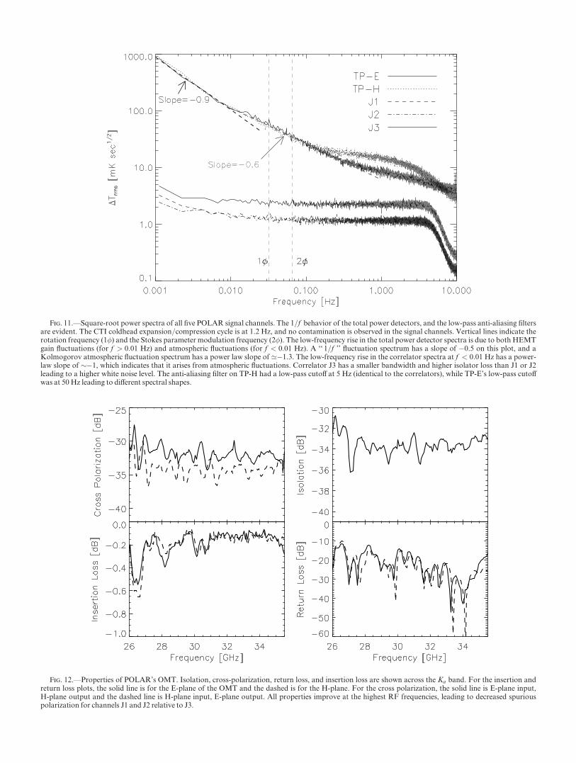
Fig. 11.—Square-root power spectra of all five POLAR signal channels. The 1=f behavior of the total power detectors, and the low-pass anti-aliasing filtersare evident. The CTI coldhead expansion/compression cycle is at 1.2 Hz, and no contamination is observed in the signal channels. Vertical lines indicate therotation frequency (1�) and the Stokes parameter modulation frequency (2�). The low-frequency rise in the total power detector spectra is due to both HEMTgain fluctuations (for f > 0:01 Hz) and atmospheric fluctuations (for f < 0:01 Hz). A ‘‘ 1=f ’’ fluctuation spectrum has a slope of �0.5 on this plot, and aKolmogorov atmospheric fluctuation spectrum has a power law slope of ’�1.3. The low-frequency rise in the correlator spectra at f < 0:01 Hz has a power-law slope of ��1, which indicates that it arises from atmospheric fluctuations. Correlator J3 has a smaller bandwidth and higher isolator loss than J1 or J2leading to a higher white noise level. The anti-aliasing filter on TP-H had a low-pass cutoff at 5 Hz (identical to the correlators), while TP-E’s low-pass cutoffwas at 50 Hz leading to different spectral shapes.

Fig. 12.—Properties of POLAR’s OMT. Isolation, cross-polarization, return loss, and insertion loss are shown across the Ka band. For the insertion andreturn loss plots, the solid line is for the E-plane of the OMT and the dashed is for the H-plane. For the cross polarization, the solid line is E-plane input,H-plane output and the dashed line is H-plane input, E-plane output. All properties improve at the highest RF frequencies, leading to decreased spuriouspolarization for channels J1 and J2 relative to J3.

polarization dominates the spurious polarization, since thetotal isolation between the polarization states is the sum ofthe isolation of the OMT and cryogenic isolators on the out-put ports of the OMT. The total isolation is <50 dB. Inaddition, path length differences in the two arms leads tophase decoherence for signals reflecting off the HEMTamplifiers and propagating in the reverse direction. Thisreduces the effects of nonzero isolation to negligible levels.The atmospheric component of antenna temperature fluctu-ations at 30 GHz follows a Kolmogorov spectrum that fallsas Tatmð f Þ / f �8=3 (Carretti et al. 2001). If the experiment isnot modulated at a frequency much higher than the kneefrequency of the fluctuation spectrum, these terms will dom-inate the system NET. To perform this modulation POLARwas rotated at 0.033 Hz. Figure 11 shows the power spectraproduced by all radiometer channels, including the effects ofatmospheric fluctuations.

The stability of the offsets over a single rotation of theinstrument is crucial to the recovery of the Stokes parame-ters. Note that the behavior of the noise should be independ-ent of the phase of the reference waveform supplied to thephase-modulation lock-in detectors. The QPC are insensi-tive to correlated signals, including uncorrelated atmo-spheric emission which is spuriously correlated by theOMT. The QPC therefore show almost no 1=f noise; resid-ual 1=f noise at the ’�25 dB level is due to cross-talk in thelow-frequency electronics and the inability to perfectlymatch the phase in each arm. The QPC proved to be power-ful monitors of the intrinsic noise of the radiometer. Overthe course of the 2000 observing campaign, we found peri-ods of high offset and large offset fluctuations to be corre-lated with environmental effects, especially the occasionalformation of dew and ice on the vacuumwindow.

5.2. Optical Cross Polarization

The corrugated scalar feed horn demonstrates low cross-polarization (Clarricoats & Olver 1984). However, even foran ideal and completely symmetric feed there is always non-zero cross-polarization. For an ideal horn, the cross-polarization induced by scattering in a plane containing thepolarization axis is identically zero since there has been nopolarization conversion. This is also manifestly true for scat-tering in a plane perpendicular to the polarization axis. How-ever, using a simple geometric optics approximation it can bedemonstrated (Clarricoats & Olver 1984) that there is polar-ization conversion (cross-polarization) which varies as sin2 �and will be peaked at � ¼ 45�, 135�, 225�, 315�, where � isthe azimuthal angle in the aperture plane. The maximumcross-polarization of the feed was measured to be �40 dB(see Fig. 5). It is primarily the off-axis response in the nearsidelobes that show cross-polarization. As shown in Carrettiet al. (2001), the quadrupolar anisotropy on scales compara-ble to the FWHM is the dominant source of spuriously corre-lated response by the feed. POLAR’s vertical drift scangeometry and low sidelobe level reduced the effect of cross-polarized optical response to negligible levels.

5.3. Nonideal Correlation Radiometer Behavior

The most significant nonideal behavior of the correlationradiometer results from electrical path length mismatchbetween the input arms. From equation (9) the correlator’sDC output is proportional to cosðD��Þ, where D�� is thephase shift between the two arms of the radiometer. A 90�

phase shift therefore results in a zero signal-to-noise ratio.The path length difference DL introduces a dispersive phaseshift, D�ð�;DLÞ. Recalling that POLARmeasures the cross-correlation at � ¼ 0 lag, and assuming constant power spec-tra across the RF band for the source, beam, and radio-meter transfer functions, from equation (9) we have

Rð0Þ /Z þ�

��

~��ð�Þ~BBð�Þj ~HHj2 d�Z �oþD�RF

�o

cosD� d� : ð23Þ

The contribution of each spectral component is thusweighted by the cosine of its phase. It is therefore imperativeto accurately match the path lengths in the system. To deter-mine the phase mismatch a completely polarized signal isinjected into the OMT input. The injected signal is swept infrequency across the RF band. By measuring the frequencymodulation of the correlator spectrum by the cosD� enve-lope, the equivalent path length imbalance can be deter-mined. The path difference measurements agreed withmeasurements of the physical waveguide path difference. Tobalance the path lengths, sections of waveguide were addedto the shorter arm of the receiver. Comparing the theoreticalNET given the RF bandwidth to the measured NET, weestimate that the differential phase shift for the correlationchannels was<20�.

The remaining nonideality results from gain asymmetrybetween arms, across the band passes. These effects can becaused by mismatched bands, temperature dependence, andphase instability of the amplifiers and/or the correlator. Inpractice it is impossible to eliminate all such effects. Follow-ing Thompson et al. (1998), Table 2 estimates of the toler-able level of a few effects that could contribute to a 2.5%degradation of the signal-to-noise ratio of the correlationreceiver.

5.4. Polarimetric Offsets

In the analysis, for each rotation of the polarimeter, thecorrelator outputs are binned into rotation angle �t andfitted to

Ið�tÞ ¼ Io þ C cos �t þ S sin �t þQ cos 2�t þU sin 2�t ;

ð24Þ

where �t ¼ 2�ft and f ¼ 0:033 Hz. In addition to the Stokesparameters Q and U, the terms C and S are monitored todetermine our sensitivity to rotation-synchronous system-atic effects, and to monitor atmospheric fluctuations. Phasesensitive detection at twice the rotation frequency removesIo and other instrumental effects that are not modulated atthis frequency.

TABLE 2

Tolerances on Correlation Polarimeter Frequency

Response Variations for a 2.5% Reduction in

Signal-to-Noise Ratio (Relative between Arms)

Type of Variation Permissible Level

Gain slope (dB) ....................................... 3.5 across band

Gain sinusoidal ripple (dB) ..................... 2.9 peak-peak

Frequency band centroid offset ............... 5% of D�RF

Phase shift between bands (deg) .............. 12.8


Figure 13 shows the output of 206 co-added rotations (1hr 43 minutes of data) from the night of 2000 May 2 binnedinto a single rotation to increase the signal to noise ratio ofthe systematic effect. Fits to Io,C, S,Q, andU for these plotsresult in the Stokes parameter offsets for each channel in theinstrumental coordinate system.

The cause of the offset was carefully investigated. Ini-tially, the magnetic coupling of the cryogenic isolators tothe Earth’s field was suspected. Helmholtz coils were usedto produce a field of ’10 G at the position of the isolators.The offsets remained unchanged after 1 hour of integrationwith the coils in place. The coils were then located at fourother azimuthal positions around the Dewar and no observ-able effects were noticed.

The modulated signals were found to be consistent with acommon optical offset for each channel (as indicated by theconsistent phasing of the signals across the channels). Un-polarized flux is correlated in the receiver due to the OMT’scross polarization and imperfect isolation, causing Io 6¼ 0.The optical flux is believed to be unpolarized, but aniso-tropic, with a dipolar and quadrupolar dependence on therotation angle �t, producing spuriously polarized compo-nents Q and U. The quadrupole anisotropy is most likelycaused by the outer, reflecting, ground screen, which is asquare ‘‘ scoop ’’ centered on the Dewar axis, while the dipoleanisotropy is attributed to the feed horn being located ’3inches radially outward from the Dewar axis centerline. Thedipolar (S and C) and quadrupolar (Q and U) componentsare present at levels that are 30 dB lower than the unpolarizedoffset Io. The frequency dependence of the offset is consistentwith the OMT’s performance. Both the cross-polarizationand the isolation of the OMT degrade with decreasing RFfrequency. Therefore, since the radiometer offset is primarily

due to the OMT’s cross-polarization, the offset will be largestfor J3 since it is the lowest frequency band. Atmosphericemission that is truly polarized by the groundscreen wouldhave a spectrum that increases with frequency, contrary towhat was observed.

Table 3 presents the offsets as a function of channel forthe 2000May 2 data. The offset phase angle dependence wasroughly constant throughout the season, whereas the mag-nitudes of the offsets were correlated among channels andvaried with observing conditions; most notably humidityand atmospheric opacity. This again supports the hypo-thesis that unpolarized anisotropic atmospheric flux ispolarized by the OMT.

To be used in the cosmological data analysis, the magni-tude and phase of the offset must be stable over >4 hr time-scales. Approximately 50% of the surviving sections of datahave stable offsets for >8 hr periods of time. Our sensitivityto Stokes parameter offsets is minimized by constraining thedemodulated data to have no dependence on an overallStokes parameter offset. This is a generalization of the pro-cedure outlined in Bond, Jaffe, & Knox (1998) to treat(unpolarized) offsets for CMB temperature anisotropyexperiments. The offset removal procedure not only con-strains the final maps produced to have zero offset, but alsoaccounts for the sensitivity degradation induced by the off-set removal. The offsets are computed from maps producedfor each channel for each contiguous 3 hr block of data thatsurvives the data editing criteria (denoted as a ‘‘ section ’’).The offset for each section is determined by enforcingconsistency (within the error bars) between the maps con-structed from all sections measuring the same pixel on thesky. This induces correlations between sections of data, andbetween adjacent pixels mapped in the same section. The

Fig. 13.—Correlator outputs binned into rotation angle for 206 rotations (1 hr 43 minutes) of data obtained during observations on 2000 May 2. The DCoffset (Io ’ 100 mK) of each channel has been removed. Unpolarized offsets and Stokes parameter offsets are visible for each of the three correlator channels.The relative phasing and offset magnitudes are consistent with the model presented in x 5.4. Fits to the Stokes parameter offsets are presented in Table 3.


offset removal and data analysis procedure are discussed indetail in O’Dell (2002).

6. METEOROLOGICAL EFFECTS ANDDATA SELECTION

A variety of weather-related phenomena was encounteredduring the Spring 2000 observing campaign. We compileddata on the Pine Bluff, Wisconsin area from both theNational Weather Service and the GOES-8 satellite dataserved by the Space Sciences and Engineering Center at theUniversity ofWisconsin-Madison.27

6.1. General Atmospheric Effects

The GOES-8 data are recorded hourly, and measures a’5 km by 5 km area, within 20 km of the POLAR observa-tory. It provided the cloud cover fraction of the area, andprecipitable water vapor (PWV) column height (as well as ahost of other weather variables). Periods of high PWV cor-related with formation of dew and ice on the vacuumwindow. Astrophysical data acquired during these periodswere not used in the analysis due to the spurious correlationproduced by reflection from the dew/ice on the window.Cloud cover fraction exhibits a bimodal histogram, withmore than 35% of the time classified as ‘‘ totally clear ’’ andabout 15% of the time categorized as completely overcast.Partially cloudy days account for the other 50% of the distri-bution. POLAR’s two total power channels monitor theatmospheric zenith temperature. Figure 14 presents a histo-gram of daily atmospheric zenith temperature measuredover the observing season by POLAR.

6.2. Solar and Lunar Effects

Based on the geometry of the inner, corotating, conicalgroundscreen, some solar radiation will enter this screenwhen sunlight propagates over the outer (fixed) ground-screen. This happens at a solar elevation of ’10�. However,for this light to enter the horn, it must scatter many times off

the inner ground screen and will then be absorbed by theinner screen’s Eccosorb coating. Below this elevation of 10�,solar radiation must undergo a double diffraction to enterthe system. The amount of sunlight in the beam-patternsteeply increases as the Sun rises until the Sun’s elevationreaches ’49�, at which time radiation from the Sun candirectly enter the horn. We found that, in practice, solarcontamination was undetectable below a solar elevation of30�. To be conservative, we eliminated all data taken withthe Sun more than 20� above the horizon. Since data werecollected 24 hours per day, this represents a sizeable 38.6%of our data, or’288 hr.

The Moon is a bright microwave source, correspondingroughly to a thermodynamic temperature of 220K. Its emis-sion is dependent upon frequency, lunar phase, and polar-ization. Using the lunar emission model presented in Keihm(1983), the COBE team calculate the lunar emission in bothpolarization states at 30, 50, and 90 GHz and show that thepolarized lunar antenna temperature at 31 GHz is d1 K(Bennett et al. 1992). Using a variation of this model, andthe POLAR beam patterns, we have estimated the polarizedantenna temperature of the Moon as a function of elevation

TABLE 3

Polar Offsets 2000 May 2: 206 Rotations (1 hour 43 Minutes of Data) Co-added and Binned into Rotation Angle

ChannelaIo

b

(mK)

C c

(lK)

S d

(lK)

Qe

(lK)

U f

(lK)

Pg

(lK)

�h

(deg)

J3I................ 133.8 1.0 75.4 38.0 �31.7 38.0 �236.3 38.0 �73.6 38.0 247.5 47.6 8.7 4.7

J2I................ 83.6 1.0 76.2 20.0 �91.3 20.0 �125.8 20.0 �25.9 20.0 128.4 23.6 5.8 4.6

J1I................ 88.1 1.0 108.3 20.0 �48.4 20.0 �99.3 20.0 21.0 20.0 101.5 23.7 �6.0 5.8

J3Q .............. 15.76 0.09 13.8 38.0 15.0 38.0 8.4 38.0 68.9 38.0 69.5 42.1 41.7 52.5

J2Q .............. 5.57 0.05 �9.6 20.0 �25.3 20.0 29.6 20.0 �28.0 20.0 41.0 28.3 �22.5 22.9

J1Q .............. 7.15 0.04 7.3 20.0 �19.1 20.0 �20.3 20.0 12.7 20.0 23.8 27.7 �16.5 31.5

Note.—Refer to Fig. 13 for data.a ‘‘ I ’’ refers to in-phase channels; ‘‘ Q ’’ refers to quad-phase channels.b Unpolarized, unmodulated intensity.c Dipole modulated cosine term.d Dipole modulated sine term.e Quadrupole modulatedQ term.f Quadrupole modulatedU term.g Magnitude of polarized offset P ¼ Q2 þU2ð Þ1=2. Over the course of the observing season, the offsets were always in the order

PðJ3Þ > PðJ2Þ > PðJ1Þ.h Phase angle of polarized offset � ¼ 1

2 tan�1 U=Qð Þ. Throughout the season, the phase angles of the offsets were roughly constant for the

in-phase channels.

27 See http://www.ssec.wisc.edu.Fig. 14.—Daily atmospheric zenith antenna temperature distribution

for the Spring 2000 observing campaign.


angle. During the Spring 2000 observing season the highestlunar elevation was 68=4. We removed all data when theMoon was more than 50� in elevation; this corresponds toabout 1.2% of the data and reduces the maximum lunar con-tribution to be<5 lK.

6.3. Atmospheric Data Cut

The primary data quality cut for selecting astrophysicaldata is based on the statistics of the S and C terms of fitsto equation (24). This cut is referred to as the 1� cut. Aspreviously mentioned, the S and C components are statisti-cally independent from the Q and U components. Since the1� component probes the power spectrum of the radio-meter at lower frequencies, it is more susceptible to con-tamination by atmospheric fluctuations and can thereforebe used as an unbiased probe of data quality which is inde-pendent of the astrophysical data. For each 7.5 minutesegment of data, the fluctuations in S and C are comparedto (1) the expected fluctuation level from Gaussian whitenoise and (2) fluctuations in S and C from the QPC which,as mentioned, display pure white noise power spectraldensities with amplitude equal to the radiometer NET.Figure 15 shows the distribution of fluctuations in the 2�component for the 7.5 minute averages for channel J2, forthe Spring 2000 observing campaign. Also indicated arethe cut levels used in the analysis presented in Keating etal. (2001) and the in-phase channel (IPC) distribution afterthe 1� cut has been applied.

7. SUMMARY

We have described the design and performance of anovel instrument that was recently used to set upper limitson the polarization of the CMB. The simplicity of the opti-cal design of the polarimeter and the observing strategyresulted in minimal systematic effects. Observations wereconducted from a convenient location near the University

of Wisconsin—Madison. The site was useful for work at30 GHz, and its proximity afforded us the ability to diag-nose problems and make rapid adjustments to optimizeinstrumental performance while still in the field. While noevidence for CMB polarization was detected with POLAR,the upper limits are impressive given the brief observingseason available during Spring 2000. This is attributable tothe low noise of the HEMT amplifier front-end andthe modest modulation requirements permitted by the sta-ble correlation radiometer back end. POLAR has provento be extremely versatile. Starting in 2001 January thePOLAR radiometer has been used as the receiver in asearch for CMB polarization at small angular scales: Cos-mic Microwave Polarization at Small Scales (COMPASS).Results from COMPASS are forthcoming and will furtherdemonstrate the viability of the correlation polarimetertechnique.

We are grateful to a number of people who influenced thedesign and analysis of POLAR. Initial theoretical guidanceand encouragement came from Alex Polnarev and RobertBrandenberger. Dick Bond, Robert Crittenden, Angelicade Oliveira-Costa, Wayne Hu, Lloyd Knox, ArthurKosowsky, Kin-Wang Ng, and Matias Zaldarriaga pro-vided crucial insight during the development and analysisphases, and vastly enhanced the scientific impact of the proj-ect. We are also indebted to several experimentalists whoworked on, supported, or guided, the construction of theinstrument: Brendan Crill, Khurram Farooqui, Kip Hyatt,Slade Klawikowski, Alan Levy, Phil Lubin, Melvin Phua,Dan Swetz, David Wilkinson, Grant Wilson, and EdWollack. B. G. K. and C. W. O. were supported by NASAGSRP Fellowships. POLAR’s HEMT amplifiers were pro-vided by John Carlstrom. This work has been supported byNSF grants AST 93-18727, AST 98-02851, and AST 00-71213, andNASA grant NAG5-9194.

Fig. 15.—Distribution of correlator fluctuations for 7.5 minute averages, as a function of cut level. The solid (black) curve shows the fluctuation level attwice the rotation frequency, relative to the NET of the system, for the in-phase channel J2I, after cuts removing Sun, Moon, and dew contamination havebeen applied. The dotted curve shows the same information, but after the 1� cut has been applied. This cut removes a large number of high-level outliers, butmuch of the remaining data still are contaminated. The dashed curve shows the distribution after all cuts have been applied; very little if any 2� contaminationremains.


REFERENCES

Bennett, C. L., et al. 1992, ApJ, 391, 466Bond, J. R., Jaffe, A. H., &Knox, L. 1998, Phys. Rev. D, 57, 2117Carretti, E., et al. 2001, NewA, 6, 173Cheng, E., et al. 1979, ApJ, 232, L139Chu, T. 1975, Bell Sys. Tech. J., 54, 1665Clarricoats, P., & Olver, A. 1984, Corrugated Horns for MicrowaveAntennas (London: Peter Peregrinus)

Fujimoto, K. 1964, IEEE-MTT,March, 233Gasiewski, A., &Kunkee, D. 1993, IEEE-MTT, 41, 767Goldsmith, P. 1998, Quasioptical Systems (NewYork: IEEE Press)Jackson, J. D. 1975, Classical Electrodynamics (NewYork:Wiley)Janssen,M. A., et al. 1979, IEEETrans. Antennas Prop., 27(4), 551Johnson, D., &Wilkinson, D. 1987, ApJ, 313, L1Kamionkowski, M., Kosowsky, A., & Stebbins, A. 1997, Phys. Rev. D, 55,7368

Keating, B., Polnarev, A., Steinberger, J., & Timbie, P. 1998, ApJ, 495, 580Keating, B., et al. 2001, ApJ, 560, L1Keihm, S. J. 1983, Planetary Sci. Inst. Rep., KKraus, J. 1986, Radio Astronomy (NewYork:McGraw-Hill)Lubin, P., & Smoot, G. 1981, ApJ, 245, L51Mason, B., et al. 1999, AJ, 118, 2908

Nanos, G. 1979, ApJ, 232, 341O’Dell, C. W. 2002, Ph.D. thesis, Univ. Wisconsin—Madison (astro-ph0201224)

O’Dell, C.W., Swetz, D. S., & Timbie, P. T. 2002, IEEE-MTT, 50, 2135Pospieszalski, M. 1992, IEEEMTT-SDigest, 1369Pozar, D. 1990,Microwave Engineering (NewYork: Addison-Wesley)Rohlfs, K. 1996, Tools of Radio Astronomy (NewYork: Springer)Sironi, G., et al. 1997, NewA, 3, 1Thompson et al. 1998, Interferometry and Synthesis in Radio Astronomy(Malabar: Krieger)

Timbie, P., &Wilkinson, D. 1990, ApJ, 353, 140Wang, X., Tegmark, M., & Zaldarriaga, M. 2001, preprint (astro-ph/0105091)

Wollack, E. J. 1995, Rev. Sci. Inst., 66, 4305Wollack, E. J., et al. 1997, ApJ, 476, 440Zaldarriaga,M. 1997, Phys. Rev. D, 55, 1822———. 1998, ApJ, 503, 1Zaldarriaga,M., & Seljak, U. 1997, Phys. Rev. D, 55, 1830Zaldarriaga,M., Spergel, D., & Seljak, U. 1997, ApJ, 488, 1Zhang, X., et al. 1993, IEEE-MTT, 41, 8

20 KEATING ET AL.

BrianG.Keating,1 ChristopherW.O’Dell,...

Documents

Transcript of BrianG.Keating,1 ChristopherW.O’Dell,...