1

Chapter 8

NUMERICAL SOLUTION

OF

ORDINARY DIFFERENTIAL EQUATIONS

2

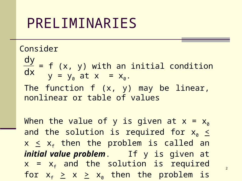
PRELIMINARIES

= f (x, y) with an initial condition y = y0 at x = x0. dx

dyConsider

The function f (x, y) may be linear, nonlinear or table of values

When the value of y is given at x = x0 and the solution is required for x0 < x < xf then the problem is called an initial value problem. If y is given at x = xf and the solution is required for xf > x > x0 then the problem is called a boundary value problem.

3

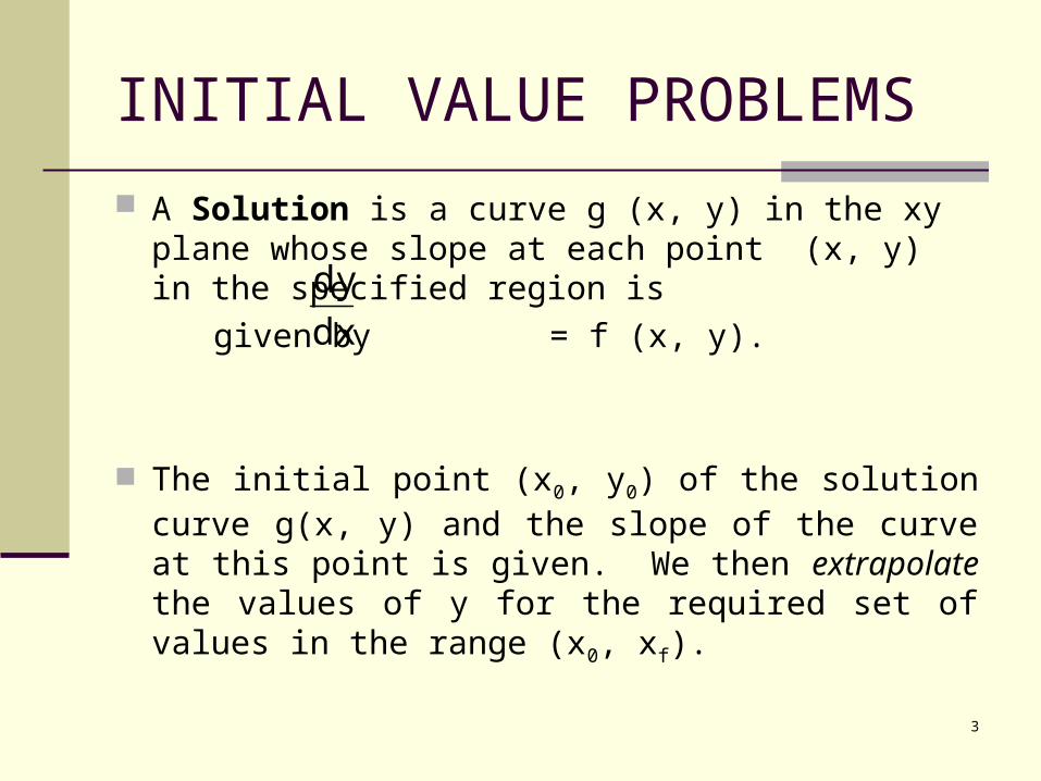
INITIAL VALUE PROBLEMS

A Solution is a curve g (x, y) in the xy plane whose slope at each point (x, y) in the specified region is

given by = f (x, y).

The initial point (x0, y0) of the solution curve g(x, y) and the slope of the curve at this point is given. We then extrapolate the values of y for the required set of values in the range (x0, xf).

dx

dy

4

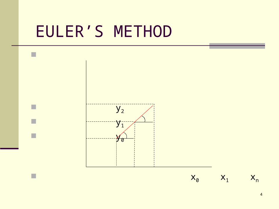
y2

y1

y0

x0 x1 xn

EULER’S METHOD

5

EULER’S METHOD

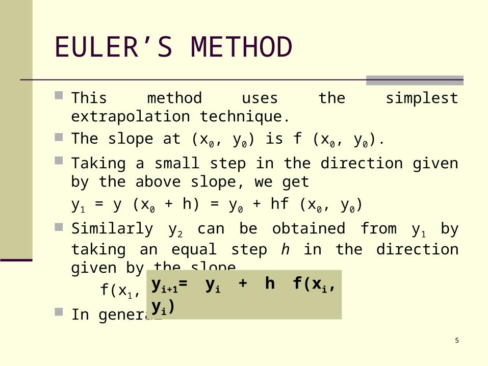
This method uses the simplest extrapolation technique.

The slope at (x0, y0) is f (x0, y0).

Taking a small step in the direction given by the above slope, we get

y1 = y (x0 + h) = y0 + hf (x0, y0)

Similarly y2 can be obtained from y1 by taking an equal step h in the direction given by the slope

f(x1, y1).

In generalyi+1= yi + h f(xi, yi)

6

Modifications

Modified Euler Method● In this method the average of the slopes at (x0, y0) and (x1, y=1

(1)) is taken instead of the slope at (x0, y0) where y1

(1) = y1 + h f (x0, y0).● In general,

Improved Modified Euler Method● In this method points are averaged instead of

slopes.

yi+1 = yi + ½ h [f (xi, yi) + f (xi + h, yi + hf (xi, yi)) ]

yi+1 = yi + hf (xi + h

2, yi +

2

h f (xi, yi) )

7

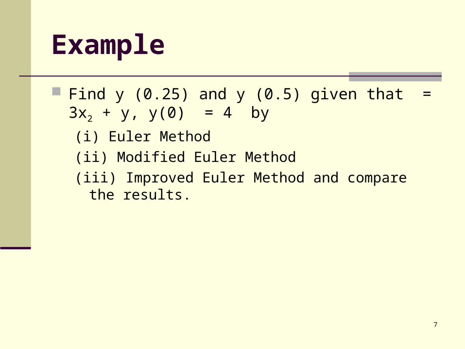
Example

Find y (0.25) and y (0.5) given that = 3x2 + y, y(0) = 4 by (i) Euler Method (ii) Modified Euler Method (iii) Improved Euler Method and compare the

results.

8

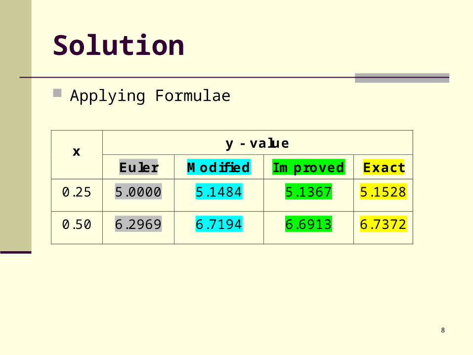
Solution

y - value x

Euler Modified Improved Exact

0.25 5.0000 5.1484 5.1367 5.1528

0.50 6.2969 6.7194 6.6913 6.7372

Applying Formulae

9

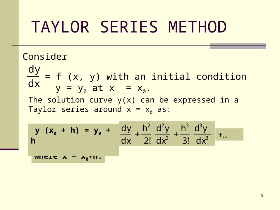
TAYLOR SERIES METHOD

= f (x, y) with an initial condition y = y0 at x = x0. dx

dyConsider

The solution curve y(x) can be expressed in a Taylor series around x = x0 as:

dx

yd

!3

h

dx

yd

!2

h

dx

dy3

33

2

22

+…

where x = x0+h.

y (x0 + h) = y0 + h

10

Example

Using Taylor series find y(0.1), y(0.2) and y(0.3) given that

= x2 - y; y(0) =1dx

dy

Solution Applying formula

y(0.1) = 0.9052y(0.2) = 0.8213 y(0.3) = 0.7492

11

PICARD’S METHOD OF SUCCESSIVE APPROXIMATIONS

This is an iterative method.

= f (x, y) with an initial condition y = y0 at x = x0. dx

dyConsider

Integrating in (x0, x0 + h) y(x0 +h) = y(x0) +

hx

x

0

0

dx)y,x(f

This integral equation is solved by successive approximations.

12

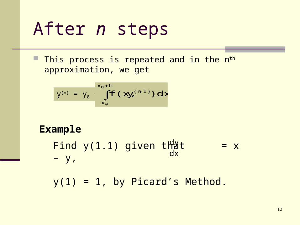
After n steps

This process is repeated and in the nth approximation, we get

y(n) = y0 +

hx

x

1)(n0

0

)dxyf(x,

Example

Find y(1.1) given that = x – y,

y(1) = 1, by Picard’s Method.

dx

dy

13

Solution

y(1)1.1 = 1 +

1.1

1

)1( dxx

= 1.005

Successive iterations yield 1.0045, 1.0046 , 1.0046

Exact value is y (1.1) = 1.0048

Thus y (1.1) = 1.0046

14

RUNGE–KUTTA METHODS

Euler Method is not very powerful in practical problems, as it requires very small step size h for reasonable accuracy.

In Taylor’s method, determination of higher order derivatives are

involved.

The Runge–Kutta methods give greater accuracy without the need to calculate higher derivatives.

15

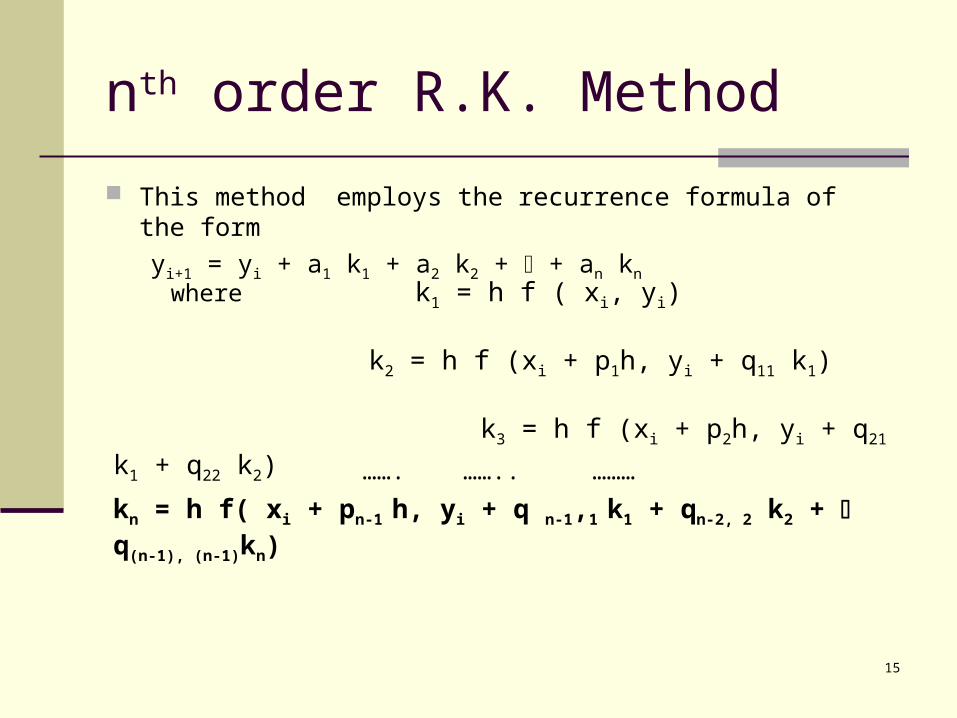
nth order R.K. Method

This method employs the recurrence formula of the form

yi+1 = yi + a1 k1 + a2 k2 + + an kn

where k1 = h f ( xi, yi)

k2 = h f (xi + p1h, yi + q11 k1)

k3 = h f (xi + p2h, yi + q21 k1 + q22 k2)

kn = h f( xi + pn-1 h, yi + q n-1,1 k1 + qn-2, 2 k2 + q(n-1), (n-1)kn)

……. …….. ………

16

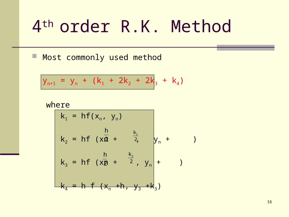
4th order R.K. Method

Most commonly used method

yn+1 = yn + (k1 + 2k2 + 2k3 + k4)

wherek1 = hf(xn, yn)

k2 = hf (xn + , yn + )

k3 = hf (xn + , yn + )

k4 = h f (xn +h, y3 +k3)

2

h

2

h

2

k1

2

k 2

17

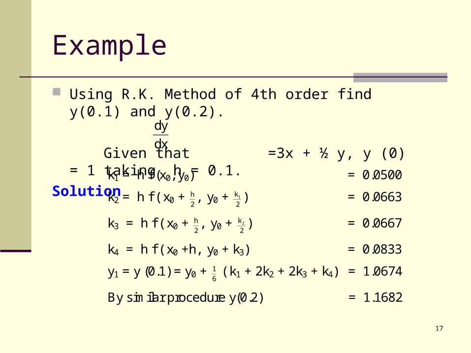
Example

Using R.K. Method of 4th order find y(0.1) and y(0.2).

Given that =3x + ½ y, y (0) = 1 taking h = 0.1.

Solution

dy

dx

k1 = h f (x0, y0) = 0.0500

k2 = h f ( x0 + 2

h , y0 + 2

k1 ) = 0.0663

k3 = h f ( x0 + 2

h , y0 + 2

k 2 ) = 0.0667

k4 = h f ( x0 +h, y0 + k3) = 0.0833

y1 = y (0.1) = y0 + 6

1 ( k1 + 2k2 + 2k3 + k4) = 1.0674

By similar procedure y(0.2) = 1.1682

18

PREDICTOR CORRECTOR METHODS

In the Runge-Kutta methods the solution, point yn+1 is evaluated using only the solution point yn and none of the previous points yn-1, yn-2 etc. on the solution curve. The behaviour of the solution in the past are ignored and each step starts afresh. This will be inefficient. The Predictor-Corrector methods take the previous solution points also into account. In these methods

● First a predictor formula is obtained and a corrector is obtained.

19

Milne’s Predictor-Corrector Method This method uses the past 4 points in the solution.

Predictor formula:

yi+1=yi-3+43

h (2fi–fi-1+2fi-2)+O(h5)

Corrector formula:

yi+1=yi-1+3

h (fi+1 + 4fi + fi-1)+O(h5).

Note: If there is a significant difference between predictor and corrector value the corrector value may be taken as predictor value and a new corrector value may be calculated.

20

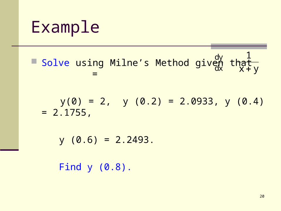
Example

Solve using Milne’s Method given that =

y(0) = 2, y (0.2) = 2.0933, y (0.4) = 2.1755,

y (0.6) = 2.2493.

Find y (0.8).

dy

dx y x

1

21

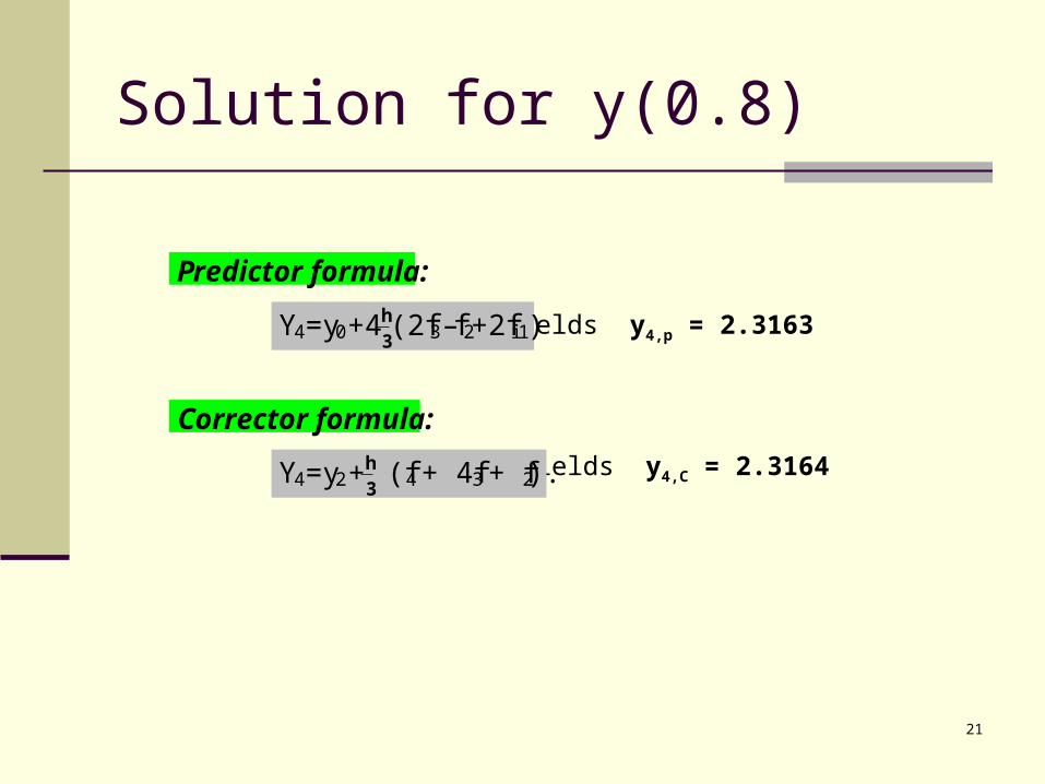
Solution for y(0.8)

yields y4,p = 2.3163

yields y4,C = 2.3164

Predictor formula:

Y4=y0+43h (2f3–f2+2fi1)

Corrector formula:

Y4=y2+3h (f4 + 4f3 + f2).

22

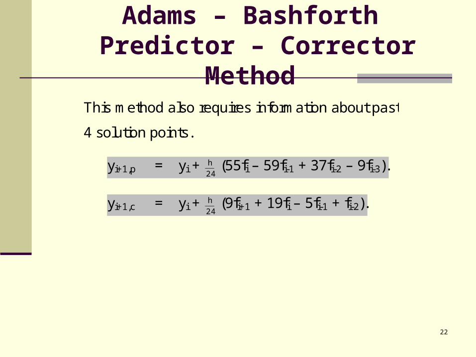
Adams – Bashforth Predictor – Corrector Method

This method also requires information about past

4 solution points.

yi+1,p = yi + 24

h (55fi – 59fi-1 + 37fi-2 – 9fi-3).

yi+1,c = yi + 24

h (9fi+1 + 19fi – 5fi-1 + fi-2).

23

Example

Given y = x2–y, y(0) = 1, y(0.1) = 0.90516, y(0.2) = 0.82127 and y (0.3) = 0.74918, find y (0.4) by Adams method.

Solution

y4,p = y3 + (55f3 – 59f2 + 37f1 – 9f0) = 0.6897

y4,c = y3 + (9f4 + 19f3 – 5f2 + f1) = 0.6897