1 Chapter 3 Demand Forecasting. 2 OverviewOverview l Introduction l Qualitative Forecasting Methods...

1

Chapter 3Chapter 3Chapter 3Chapter 3

Demand ForecastingDemand Forecasting

2

OverviewOverviewOverviewOverview

IntroductionIntroduction Qualitative Forecasting MethodsQualitative Forecasting Methods Quantitative Forecasting ModelsQuantitative Forecasting Models How to Have a Successful Forecasting SystemHow to Have a Successful Forecasting System Computer Software for ForecastingComputer Software for Forecasting

3

Introduction Introduction Introduction Introduction

Demand estimatesDemand estimates for products and services are the for products and services are the starting point for all the other planning in operations starting point for all the other planning in operations management.management.

Forecasting integral to production planning.Forecasting integral to production planning. Long-range survival, growth, and profitability Long-range survival, growth, and profitability as well as well

as as short-range efficiency and effectiveness short-range efficiency and effectiveness depend on depend on accurate forecasting.accurate forecasting.

4

Forecasting is an Integral PartForecasting is an Integral Part of Business Planning of Business Planning

Forecasting is an Integral PartForecasting is an Integral Part of Business Planning of Business Planning

ForecastForecastMethod(s)Method(s)

DemandDemandEstimatesEstimates

SalesSalesForecastForecast

ManagementManagementTeamTeam

Inputs:Inputs:Market,Market,

Economic,Economic,OtherOther

BusinessBusinessStrategyStrategy

Production ResourceProduction ResourceForecastsForecasts

5

Some Reasons WhySome Reasons WhyForecasting is Essential in OMForecasting is Essential in OM

Some Reasons WhySome Reasons WhyForecasting is Essential in OMForecasting is Essential in OM

New Facility PlanningNew Facility Planning requires long-range forecasts requires long-range forecasts – – It can take 5 years to design and build a new factory It can take 5 years to design and build a new factory or design and implement a new production process.or design and implement a new production process.

Production PlanningProduction Planning requires medium-range forecasts requires medium-range forecasts – Demand for products vary from month to month – Demand for products vary from month to month and it can take several months to change the and it can take several months to change the capacities of production processes.capacities of production processes.

Workforce SchedulingWorkforce Scheduling requires short-range forecastsrequires short-range forecasts – Demand for services (and the necessary staffing) – Demand for services (and the necessary staffing) can vary from hour to hour and employees weekly can vary from hour to hour and employees weekly work schedules must be developed in advance.work schedules must be developed in advance.

6

Examples of Production Resource ForecastsExamples of Production Resource ForecastsExamples of Production Resource ForecastsExamples of Production Resource Forecasts

LongLongRangeRange

MediumMediumRangeRange

ShortShortRangeRange

YearsYears

MonthsMonths

Days,Days,WeeksWeeks

Product Lines,Product Lines,Factory CapacitiesFactory Capacities

ForecastForecastHorizonHorizon

TimeTimeSpanSpan

Item BeingItem BeingForecastedForecasted

Unit ofUnit ofMeasureMeasure

Product Groups,Product Groups,Depart. CapacitiesDepart. Capacities

Specific Products,Specific Products,Machine CapacitiesMachine Capacities

Dollars,Dollars,TonsTons

Units,Units,PoundsPounds

Units,Units,HoursHours

7

Forecasting MethodsForecasting MethodsForecasting MethodsForecasting Methods

Qualitative ApproachesQualitative Approaches Quantitative ApproachesQuantitative Approaches

8

Qualitative ApproachesQualitative ApproachesQualitative ApproachesQualitative Approaches

Usually based on judgments about causal factors that Usually based on judgments about causal factors that underlie the demand of particular products or servicesunderlie the demand of particular products or services

Do not require a demand history for the product or Do not require a demand history for the product or service, therefore are useful for new products/servicesservice, therefore are useful for new products/services

Approaches vary in sophistication from scientifically Approaches vary in sophistication from scientifically conducted surveys to intuitive hunches about future conducted surveys to intuitive hunches about future eventsevents

The approach/method that is appropriate depends on The approach/method that is appropriate depends on a product’s life cycle stagea product’s life cycle stage

9

Qualitative Methods Qualitative Methods Qualitative Methods Qualitative Methods

Educated guessEducated guess intuitive hunchesintuitive hunches Executive committee consensusExecutive committee consensus Delphi methodDelphi method Survey of sales forceSurvey of sales force Survey of customers Survey of customers Historical analogyHistorical analogy Market researchMarket research sscientifically conducted cientifically conducted

surveyssurveys

10

Quantitative Forecasting ApproachesQuantitative Forecasting ApproachesQuantitative Forecasting ApproachesQuantitative Forecasting Approaches

Based on the assumption that the “forces” that Based on the assumption that the “forces” that generated the past demand will generate the future generated the past demand will generate the future demand, i.e., history will tend to repeat itselfdemand, i.e., history will tend to repeat itself

Analysis of the past demand pattern provides a good Analysis of the past demand pattern provides a good basis for forecasting future demandbasis for forecasting future demand

Majority of quantitative approaches fall in the Majority of quantitative approaches fall in the category of time series analysiscategory of time series analysis

11

A A time seriestime series is a set of numbers where the order or is a set of numbers where the order or sequence of the numbers is important, e.g., historical sequence of the numbers is important, e.g., historical demanddemand

Analysis of the time series identifies patternsAnalysis of the time series identifies patterns Once the patterns are identified, Once the patterns are identified, an appropriate an appropriate

method method can be used can be used to develop a forecastto develop a forecast

Time Series AnalysisTime Series AnalysisTime Series AnalysisTime Series Analysis

12

Components of a Time Series Components of a Time Series Components of a Time Series Components of a Time Series

TrendsTrends are noted by an upward or downward sloping are noted by an upward or downward sloping line.line.

CycleCycle is a data pattern that may cover several years is a data pattern that may cover several years before it repeats itself.before it repeats itself.

SeasonalitySeasonality is a data pattern that repeats itself over is a data pattern that repeats itself over the period of one year or less.the period of one year or less.

Random fluctuation (noise)Random fluctuation (noise) results from random results from random variation or unexplained causes.variation or unexplained causes.

14

Product Demand Charted over 4 Years with Product Demand Charted over 4 Years with Trend and SeasonalityTrend and Seasonality

Product Demand Charted over 4 Years with Product Demand Charted over 4 Years with Trend and SeasonalityTrend and Seasonality

Year1

Year2

Year3

Year4

Seasonal peaks Trend component

Actual demand line

Average demand over four years

Dem

and

for p

rodu

ct o

r ser

vice

Random variation

15

Seasonal PatternsSeasonal PatternsSeasonal PatternsSeasonal Patterns

Length of TimeLength of Time Number of Number of

Before Pattern Length ofBefore Pattern Length of Seasons Seasons

Is RepeatedIs Repeated Season Season in Pattern in Pattern

YearYear QuarterQuarter 4 4

YearYear Month Month 1212

YearYear Week Week 5252

MonthMonth Day Day 28-31 28-31

WeekWeek Day Day 7 7

16

Quantitative Forecasting ApproachesQuantitative Forecasting ApproachesQuantitative Forecasting ApproachesQuantitative Forecasting Approaches

Linear RegressionLinear Regression Simple Moving AverageSimple Moving Average Weighted Moving AverageWeighted Moving Average Exponential Smoothing (exponentially weighted Exponential Smoothing (exponentially weighted

moving average)moving average) Exponential Smoothing with Trend (double Exponential Smoothing with Trend (double

exponential smoothing)exponential smoothing)

17

Long-Range ForecastsLong-Range ForecastsLong-Range ForecastsLong-Range Forecasts

Time spans usually greater than one yearTime spans usually greater than one year Necessary to support strategic decisions about Necessary to support strategic decisions about

planning products, processes, and facilitiesplanning products, processes, and facilities For long-range forecasting, it is important to plot For long-range forecasting, it is important to plot

historical time series data in order to identify data historical time series data in order to identify data patterns (trends, cycles, seasonality) so that a proper patterns (trends, cycles, seasonality) so that a proper forecasting method can be used.forecasting method can be used.

18

Simple Linear RegressionSimple Linear RegressionSimple Linear RegressionSimple Linear Regression

Linear regression analysis establishes a relationship Linear regression analysis establishes a relationship between a dependent variable and one or more between a dependent variable and one or more independent variables.independent variables.

In In simple linear regression analysissimple linear regression analysis there is only one there is only one independent variable.independent variable.

If If the data is a time series, the independent variable the data is a time series, the independent variable is the time period.is the time period.

The dependent variable is whatever we wish to The dependent variable is whatever we wish to forecast.forecast.

19


Regression EquationRegression Equation

This model is of the form:This model is of the form:

Y = a + bXY = a + bX

Y = dependent variableY = dependent variable

X = independent variableX = independent variable

a = y-axis intercepta = y-axis intercept ( (the height of the the height of the line when x = 0line when x = 0))

b = slope of regression line b = slope of regression line which which is is the amount by which y increases when x increasethe amount by which y increases when x increasess by 1 unit.by 1 unit.

20


Constants a and bConstants a and b

The constants a and b are computed using the The constants a and b are computed using the following equations:following equations:

2

2 2

x y- x xya =

n x -( x)

2 2

xy- x yb =

n x -( x)

n

21


Once the a and b values are computed, a future value Once the a and b values are computed, a future value of X can be entered into the regression equation and a of X can be entered into the regression equation and a corresponding value of Y (the forecast) can be corresponding value of Y (the forecast) can be calculated.calculated.

22

Example: College EnrollmentExample: College EnrollmentExample: College EnrollmentExample: College Enrollment

Simple Linear RegressionSimple Linear Regression

At a small regional college enrollments have grown At a small regional college enrollments have grown steadily over the past six years, as evidenced below. steadily over the past six years, as evidenced below. Use time series regression to forecast the student Use time series regression to forecast the student enrollments for the next three years. enrollments for the next three years.

StudentsStudents StudentsStudentsYearYear Enrolled (1000s)Enrolled (1000s) YearYear Enrolled (1000s)Enrolled (1000s) 11 2.52.5 44 3.23.2 22 2.82.8 55 3.33.3 33 2.92.9 66 3.43.4

23



xx yy xx22 xyxy11 2.52.5 11 2.52.522 2.82.8 44 5.65.633 2.92.9 99 8.78.744 3.23.2 1616 12.812.855 3.33.3 2525 16.516.566 3.43.4 3636 20.420.4

x=21 x=21 y=18.1 y=18.1 xx22=91 =91 xy=66.5xy=66.5

24



Y = 2.387 + 0.180XY = 2.387 + 0.180X

2

91(18.1) 21(66.5)2.387

6(91) (21)a

6(66.5) 21(18.1)0.180

105b

25



YY77 = 2.387 + 0.180(7) = 3.65 or 3,650 students = 2.387 + 0.180(7) = 3.65 or 3,650 students



Note: Enrollment is expected to increase by 180Note: Enrollment is expected to increase by 180 students per year.students per year.

26


Simple linear regression can also be used when the Simple linear regression can also be used when the independent variable X represents a variable other independent variable X represents a variable other than time.than time.

In this case, linear regression is representative of a In this case, linear regression is representative of a class of forecasting models called class of forecasting models called causal forecasting causal forecasting modelsmodels..

27

Example: Railroad Products Co.Example: Railroad Products Co.Example: Railroad Products Co.Example: Railroad Products Co.

Simple Linear Regression – Causal ModelSimple Linear Regression – Causal Model

The manager of RPC wants to project the sales The manager of RPC wants to project the sales for the next 3 years. He knows that RPC’s long-for the next 3 years. He knows that RPC’s long-range sales are tied very closely to national freight car range sales are tied very closely to national freight car loadings. On the next slide are 7 years of relevant loadings. On the next slide are 7 years of relevant historical data.historical data.

Develop a simple linear regression model Develop a simple linear regression model between RPC sales and national freight car loadings. between RPC sales and national freight car loadings. Forecast RPC sales for the next 3 years, given that the Forecast RPC sales for the next 3 years, given that the rail industry estimates car loadings of 250, 270, and rail industry estimates car loadings of 250, 270, and 300 million.300 million.

28



RPC SalesRPC Sales Car LoadingsCar Loadings

YearYear ($millions)($millions) (millions)(millions)11 9.59.5 12012022 11.011.0 13513533 12.012.0 13013044 12.512.5 15015055 14.014.0 17017066 16.016.0 19019077 18.018.0 220220

29



xx yy xx22 xyxy

120120 9.59.5 14,40014,400 1,1401,140135135 11.011.0 18,22518,225 1,4851,485130130 12.012.0 16,90016,900 1,5601,560150150 12.512.5 22,50022,500 1,8751,875170170 14.014.0 28,90028,900 2,3802,380190190 16.016.0 36,10036,100 3,0403,040220220 18.018.0 48,40048,400 3,9603,960

1,1151,115 93.093.0 185,425185,425 15,44015,440

30



Y = 0.528 + 0.0801XY = 0.528 + 0.0801X

2

185,425(93) 1,115(15,440)a 0.528

7(185,425) (1,115)

2

7(15,440) 1,115(93)b 0.0801

7(185,425) (1,115)

31



YY8 8 = 0.528 + 0.0801(250) = $20.55 million = 0.528 + 0.0801(250) = $20.55 million

YY9 9 = 0.528 + 0.0801(270) = $22.16 million = 0.528 + 0.0801(270) = $22.16 million

YY1010 = 0.528 + 0.0801(300) = $24.56 million = 0.528 + 0.0801(300) = $24.56 million

Note: RPC sales are expected to increase by Note: RPC sales are expected to increase by $80,100 for each additional million national freight $80,100 for each additional million national freight car loadings.car loadings.

32

Multiple Regression AnalysisMultiple Regression AnalysisMultiple Regression AnalysisMultiple Regression Analysis

Multiple regression analysis is used when there are Multiple regression analysis is used when there are two or more independent variables.two or more independent variables.

An example of a multiple regression equation is:An example of a multiple regression equation is:

Y = 50.0 + 0.05XY = 50.0 + 0.05X11 + 0.10X + 0.10X22 – 0.03X – 0.03X33

where: Y = firm’s annual sales ($millions)where: Y = firm’s annual sales ($millions)

XX11 = industry sales ($millions) = industry sales ($millions)

XX22 = regional per capita income = regional per capita income

($thousands)($thousands)

XX33 = regional per capita debt ($thousands) = regional per capita debt ($thousands)

33

Coefficient of Correlation (Coefficient of Correlation (rr))Coefficient of Correlation (Coefficient of Correlation (rr))

The coefficient of correlation, The coefficient of correlation, rr, explains the relative , explains the relative importance of the relationship between importance of the relationship between xx and and yy..

The sign of The sign of rr shows the direction of the relationship. shows the direction of the relationship. The absolute value of The absolute value of rr shows the strength of the shows the strength of the

relationship.relationship. The sign of The sign of rr is always the same as the sign of b. is always the same as the sign of b. rr can take on any value between –1 and +1. can take on any value between –1 and +1.

34


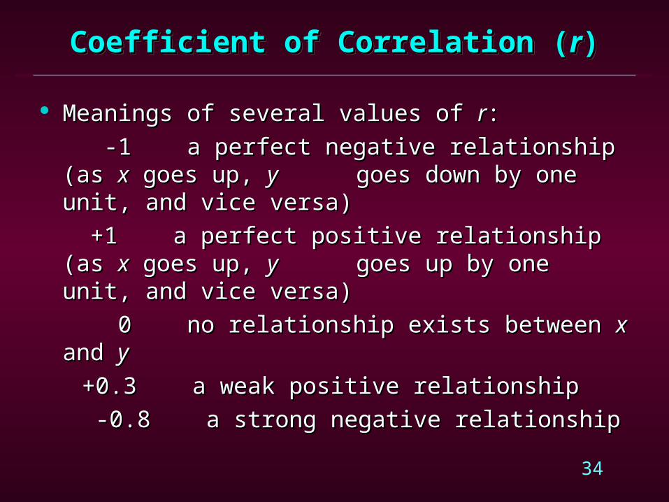
Meanings of several values of Meanings of several values of rr::

-1 a perfect negative relationship (as -1 a perfect negative relationship (as xx goes up, goes up, yy goes down by one unit, and vice versa) goes down by one unit, and vice versa)

+1 a perfect positive relationship (as +1 a perfect positive relationship (as xx goes up, goes up, yy goes up by one unit, and vice versa) goes up by one unit, and vice versa)

0 no relationship exists between 0 no relationship exists between xx and and yy

+0.3 a weak positive relationship+0.3 a weak positive relationship

-0.8 a strong negative relationship-0.8 a strong negative relationship

35


r r is computed by: is computed by:

2 2 2 2( ) ( )

n xy x yr

n x x n y y

2 2 2 2( ) ( )

n xy x yr

n x x n y y

36

Coefficient of Determination (Coefficient of Determination (rr22))Coefficient of Determination (Coefficient of Determination (rr22))

The coefficient of determination, The coefficient of determination, rr22, is the square of , is the square of the coefficient of correlation.the coefficient of correlation.

The modification of The modification of rr to to rr22 allows us to shift from allows us to shift from subjective measures of relationship to a more specific subjective measures of relationship to a more specific measure.measure.

rr22 is determined by the ratio of explained variation to is determined by the ratio of explained variation to total variation:total variation:

22

2

( )

( )

Y yr

y y

22

2

( )

( )

Y yr

y y

37


The The coefficient of determination, r coefficient of determination, r 22,, is useful because it gives is useful because it gives the proportion of the variance (fluctuation) of one variable the proportion of the variance (fluctuation) of one variable that is predictable from the other that is predictable from the other vvariable.ariable.

It is a measure that allows us to determine how certain one It is a measure that allows us to determine how certain one can be in making predictions from a certain model/graph.can be in making predictions from a certain model/graph.

The The coefficient of determinationcoefficient of determination is the ratio of the explained is the ratio of the explained variation to the totalvariation to the total variation.variation.

The The coefficient of determinationcoefficient of determination is such that 0 is such that 0 << rr 2 2 << 1, and 1, and denotes the strengthdenotes the strength of the linear of the linear aassociation between ssociation between xx and and yy. .

38


The The coefficient of determinationcoefficient of determination represents the percent of the represents the percent of the data that is the closestdata that is the closest to the line of best fit. For example, if to the line of best fit. For example, if rr = 0.922, then = 0.922, then r r 22 = 0.850, which means that = 0.850, which means that 85% of the total 85% of the total variation in variation in yy can be explained by the linear relationship can be explained by the linear relationship between between xx and and yy (as described by the regression (as described by the regression eequation). quation). The other 15% of the total variationThe other 15% of the total variation in in yy remains unexplained. remains unexplained.

The The coefficient of determinationcoefficient of determination is a measure of how well the is a measure of how well the regression lineregression line represents the data. If the regression line represents the data. If the regression line passes exactly through every point on thepasses exactly through every point on the scatter plot, it scatter plot, it would be able to explain all of the variation. The further the would be able to explain all of the variation. The further the line is away from the points, the less it is able to explain. line is away from the points, the less it is able to explain.

39


Coefficient of CorrelationCoefficient of Correlation

xx yy xx22 xyxy yy22

120120 9.59.5 14,40014,400 1,1401,140 90.2590.25135135 11.011.0 18,22518,225 1,4851,485 121.00121.00130130 12.012.0 16,90016,900 1,5601,560 144.00144.00150150 12.512.5 22,50022,500 1,8751,875 156.25156.25170170 14.014.0 28,90028,900 2,3802,380 196.00196.00190190 16.016.0 36,10036,100 3,0403,040 256.00256.00220220 18.018.0 48,40048,400 3,9603,960 324.00324.00

1,1151,115 93.093.0 185,425185,425 15,44015,440 1,287.501,287.50

40


Coefficient of CorrelationCoefficient of Correlation

r r = .9829 = .9829

2 2

7(15,440) 1,115(93)

7(185,425) (1,115) 7(1,287.5) (93)r

41


Coefficient of DeterminationCoefficient of Determination

rr2 2 = (.9829) = (.9829)22 = .966 = .966

96.6% of the variation in RPC sales is explained by 96.6% of the variation in RPC sales is explained by national freight car loadings.national freight car loadings.

42

Ranging ForecastsRanging ForecastsRanging ForecastsRanging Forecasts

Forecasts for future periods are only estimates and are Forecasts for future periods are only estimates and are subject to error.subject to error.

One way to deal with uncertainty is to develop best-One way to deal with uncertainty is to develop best-estimate forecasts and the estimate forecasts and the rangesranges within which the within which the actual data are likely to fall.actual data are likely to fall.

The ranges of a forecast are defined by the upper and The ranges of a forecast are defined by the upper and lower limits of a confidence interval.lower limits of a confidence interval.

43


The ranges or limits of a forecast are estimated by:The ranges or limits of a forecast are estimated by:

Upper limit = Y + t(sUpper limit = Y + t(syxyx))

Lower limit = Y - t(sLower limit = Y - t(syxyx))

where:where:

Y = best-estimate forecastY = best-estimate forecast

t = number of standard deviations from the mean t = number of standard deviations from the mean of the distribution to provide a given proba- of the distribution to provide a given probability of exceeding the limits through bility of exceeding the limits through

chancechance

ssyxyx = standard error of the forecast = standard error of the forecast

44


The The standard error (deviation) of the forecaststandard error (deviation) of the forecast is is computed as:computed as:

2

yx

y - a y - b xys =

n - 2 2

yx

y - a y - b xys =

n - 2

45


Ranging ForecastsRanging Forecasts

Recall that linear regression analysis provided Recall that linear regression analysis provided a forecast of annual sales for RPC in year 8 equal to a forecast of annual sales for RPC in year 8 equal to $20.55 million. $20.55 million.

Set the limits (ranges) of the forecast so that Set the limits (ranges) of the forecast so that there is only a 5 percent probability of exceeding the there is only a 5 percent probability of exceeding the limits by chance.limits by chance.

46


Ranging ForecastsRanging Forecasts Step 1: Compute the standard error of the Step 1: Compute the standard error of the

forecasts, s forecasts, syxyx..

Step 2: Determine the appropriate value for t.Step 2: Determine the appropriate value for t.

n = 7, so degrees of freedom = n – 2 = 5.n = 7, so degrees of freedom = n – 2 = 5.

level of significance = =.05level of significance = =.05

Appendix B, Table 2 shows t = 2.571.Appendix B, Table 2 shows t = 2.571.

1287.5 .528(93) .0801(15,440).5748

7 2yxs

47


Ranging ForecastsRanging Forecasts Step 3: Compute upper and lower limits.Step 3: Compute upper and lower limits.

Upper limit = 20.55 + 2.571(.5748)Upper limit = 20.55 + 2.571(.5748)= 20.55 + 1.478= 20.55 + 1.478= 22.028= 22.028

Lower limit = 20.55 - 2.571(.5748)Lower limit = 20.55 - 2.571(.5748)= 20.55 - 1.478= 20.55 - 1.478= 19.072= 19.072

We are 95% confident the actual sales for year 8 We are 95% confident the actual sales for year 8 will be between $19.072 and $22.028 million.will be between $19.072 and $22.028 million.

48

Seasonalized Time Series Regression AnalysisSeasonalized Time Series Regression AnalysisSeasonalized Time Series Regression AnalysisSeasonalized Time Series Regression Analysis

Select a representative historical data set.Select a representative historical data set. Develop a seasonal index for each season.Develop a seasonal index for each season. Use the seasonal indexes to deseasonalize the data.Use the seasonal indexes to deseasonalize the data. Perform lin. regr. analysis on the deseasonalized data.Perform lin. regr. analysis on the deseasonalized data. Use the regression equation to compute the forecasts.Use the regression equation to compute the forecasts. Use the seas. indexes to reapply the seasonal patterns Use the seas. indexes to reapply the seasonal patterns

to the forecasts.to the forecasts.

49

Example: Computer Products Corp.Example: Computer Products Corp.Example: Computer Products Corp.Example: Computer Products Corp.

Seasonalized Times Series Regression AnalysisSeasonalized Times Series Regression Analysis

An analyst at CPC wants to develop next year’s An analyst at CPC wants to develop next year’s quarterly forecasts of sales revenue for CPC’s line of quarterly forecasts of sales revenue for CPC’s line of Epsilon Computers. She believes that the most recent Epsilon Computers. She believes that the most recent 8 quarters of sales (shown on the next slide) are 8 quarters of sales (shown on the next slide) are representative of next year’s sales.representative of next year’s sales.

50


Seasonalized Times Series Regression AnalysisSeasonalized Times Series Regression Analysis Representative Historical Data SetRepresentative Historical Data Set

YearYear Qtr.Qtr. ($mil.)($mil.) YearYear Qtr.Qtr. ($mil.)($mil.)

11 11 7.47.4 22 11 8.38.311 22 6.56.5 22 22 7.47.411 33 4.94.9 22 33 5.45.411 44 16.116.1 22 44 18.018.0

51


Seasonalized Times Series Regression AnalysisSeasonalized Times Series Regression Analysis Compute the Seasonal IndexesCompute the Seasonal Indexes

Quarterly SalesQuarterly Sales

YearYear Q1Q1 Q2Q2 Q3Q3 Q4Q4 TotalTotal11 7.47.4 6.56.5 4.94.9 16.116.1 34.934.922 8.38.3 7.47.4 5.45.4 18.018.0 39.139.1

TotalsTotals15.715.7 13.913.9 10.310.3 34.134.1 74.074.0 Qtr. Avg.Qtr. Avg.7.857.85 6.956.95 5.155.15 17.0517.05 9.259.25

Seas.Ind.Seas.Ind..849.849 .751.751 .557.557 1.8431.843 4.0004.000

52


Seasonalized Times Series Regression AnalysisSeasonalized Times Series Regression Analysis Deseasonalize the DataDeseasonalize the Data

Quarterly SalesQuarterly Sales

YearYear Q1Q1 Q2Q2 Q3Q3 Q4Q411 8.728.72 8.668.66 8.808.80 8.748.7422 9.789.78 9.859.85 9.699.69 9.779.77

53


Seasonalized Times Series Regression AnalysisSeasonalized Times Series Regression Analysis Perform Regression on Deseasonalized DataPerform Regression on Deseasonalized Data

Yr.Yr. Qtr.Qtr. xx yy xx22 xyxy

11 11 11 8.728.72 11 8.728.7211 22 22 8.668.66 44 17.3217.3211 33 33 8.808.80 99 26.4026.4011 44 44 8.748.74 1616 34.9634.9622 11 55 9.789.78 2525 48.9048.9022 22 66 9.859.85 3636 59.1059.1022 33 77 9.699.69 4949 67.8367.8322 44 88 9.779.77 6464 78.1678.16

TotalsTotals 3636 74.0174.01 204204 341.39341.39

54


Seasonalized Times Series Regression AnalysisSeasonalized Times Series Regression Analysis Perform Regression on Deseasonalized DataPerform Regression on Deseasonalized Data

Y = 8.357 + 0.199XY = 8.357 + 0.199X

2

204(74.01) 36(341.39)a 8.357

8(204) (36)

2

8(341.39) 36(74.01)b 0.199

8(204) (36)

55


Seasonalized Times Series Regression AnalysisSeasonalized Times Series Regression Analysis Compute the Deseasonalized ForecastsCompute the Deseasonalized Forecasts

YY9 9 = 8.357 + 0.199(9) = 10.148 = 8.357 + 0.199(9) = 10.148

YY10 10 = 8.357 + 0.199(10) = 10.347 = 8.357 + 0.199(10) = 10.347

YY11 11 = 8.357 + 0.199(11) = 10.546 = 8.357 + 0.199(11) = 10.546

YY12 12 = 8.357 + 0.199(12) = 10.745 = 8.357 + 0.199(12) = 10.745

Note: Average sales are expected to increase byNote: Average sales are expected to increase by

.199 million (about $200,000) per .199 million (about $200,000) per quarter.quarter.

56


Seasonalized Times Series Regression AnalysisSeasonalized Times Series Regression Analysis Seasonalize the ForecastsSeasonalize the Forecasts

Seas.Seas. Deseas.Deseas. Seas.Seas.Yr.Yr. Qtr.Qtr. IndexIndex ForecastForecast ForecastForecast

33 11 .849.849 10.14810.148 8.628.6233 22 .751.751 10.34710.347 7.777.7733 33 .557.557 10.54610.546 5.875.8733 44 1.8431.843 10.74510.745 19.8019.80

57

Evaluating Forecast-Model PerformanceEvaluating Forecast-Model PerformanceEvaluating Forecast-Model PerformanceEvaluating Forecast-Model Performance

AccuracyAccuracy Accuracy is the typical criterion for judging the Accuracy is the typical criterion for judging the

performance of a forecasting approachperformance of a forecasting approach Accuracy is how well the forecasted values match Accuracy is how well the forecasted values match

the actual valuesthe actual values

58

Monitoring Accuracy Monitoring Accuracy Monitoring Accuracy Monitoring Accuracy

Accuracy of a forecasting approach needs to be Accuracy of a forecasting approach needs to be monitored to assess the confidence you can have in monitored to assess the confidence you can have in its forecasts and changes in the market may require its forecasts and changes in the market may require reevaluation of the approachreevaluation of the approach

Accuracy can be measured in several waysAccuracy can be measured in several ways Standard error of the forecast (sStandard error of the forecast (syyxx , ,covered earlier)covered earlier) Mean absolute deviation (MAD)Mean absolute deviation (MAD) Mean squared error (MSE)Mean squared error (MSE)

59

Monitoring AccuracyMonitoring AccuracyMonitoring AccuracyMonitoring Accuracy

Mean Absolute Deviation (MAD)Mean Absolute Deviation (MAD)

n

periodsn for deviation absolute of Sum=MAD

n

i ii=1

Actual demand -Forecast demandMAD =

n

60

Mean Squared Error (MSE)Mean Squared Error (MSE)

MSE = (SMSE = (Syxyx))22

A small value for SA small value for Syxyx means data points are means data points are

tightly grouped around the tightly grouped around the regression regression line and line and error range is small. error range is small.

When forecast errors are When forecast errors are assumed to be assumed to be normally distributed, the values of MAD and snormally distributed, the values of MAD and syxyx

are related:are related:

MSE = 1.25(MAD)MSE = 1.25(MAD)

Monitoring AccuracyMonitoring AccuracyMonitoring AccuracyMonitoring Accuracy

61

Short-Range Forecasting MethodsShort-Range Forecasting MethodsShort-Range Forecasting MethodsShort-Range Forecasting Methods

Naive MethodNaive Method (Simple) Moving Average(Simple) Moving Average Weighted Moving AverageWeighted Moving Average Exponential SmoothingExponential Smoothing Exponential Smoothing with TrendExponential Smoothing with Trend

62

Naive Method For ForecastingNaive Method For ForecastingNaive Method For ForecastingNaive Method For Forecasting

Forecasts based only on the most recent observations Forecasts based only on the most recent observations are called as “naive forecasts.”are called as “naive forecasts.”

Assumes that the next period will be identical to the Assumes that the next period will be identical to the present:present:

FFt t = A = A t-1t-1

FFtt : Forecast value for time period t : Forecast value for time period t

A A t-1t-1 : Observed value one period earlier : Observed value one period earlier

63

Simple Moving AverageSimple Moving AverageSimple Moving AverageSimple Moving Average

An averaging period (AP) is given or selectedAn averaging period (AP) is given or selected The forecast for the next period is the arithmetic The forecast for the next period is the arithmetic

average of the AP most recent actual demandsaverage of the AP most recent actual demands It is called a It is called a ““simplesimple” ” average because each average because each

period used to compute the average is equally period used to compute the average is equally weightedweighted..

64

Simple Moving AverageSimple Moving AverageSimple Moving AverageSimple Moving Average

It is called It is called ““movingmoving” ” because as new demand data because as new demand data becomes available, the oldest data is not usedbecomes available, the oldest data is not used..

By increasing the AP, the forecast By increasing the AP, the forecast can becomecan become less less responsive to fluctuations in demand responsive to fluctuations in demand

By decreasing the AP, the forecast is more responsive By decreasing the AP, the forecast is more responsive to fluctuations in demandto fluctuations in demand

65

EXAMPLE (Moving Average)EXAMPLE (Moving Average)EXAMPLE (Moving Average)EXAMPLE (Moving Average)

See example 3.5 (page 83)See example 3.5 (page 83)

66

Summary of Moving AveragesSummary of Moving AveragesSummary of Moving AveragesSummary of Moving Averages

Advantages of Moving Average MethodAdvantages of Moving Average Method Easily understoodEasily understood Easily computedEasily computed Provides stable forecastsProvides stable forecasts

Disadvantages of Moving Average MethodDisadvantages of Moving Average Method Requires saving all past N data pointsRequires saving all past N data points Lags behind a trendLags behind a trend Ignores complex relationships in dataIgnores complex relationships in data

67

Simple Moving AverageSimple Moving AverageSimple Moving AverageSimple Moving AverageFigure 3-4

MAn = n

Aii = 1n

35

37

39

41

43

45

47

1 2 3 4 5 6 7 8 9 10 11 12

Actual

MA3

MA5

68

Weighted Moving AverageWeighted Moving AverageWeighted Moving AverageWeighted Moving Average

This is a variation on the simple moving average This is a variation on the simple moving average where the weights used to compute the average are where the weights used to compute the average are not equal.not equal.

This allows more recent demand data to have a This allows more recent demand data to have a greater effect on the moving average, therefore the greater effect on the moving average, therefore the forecast.forecast.

The weights must add to 1.0 and generally The weights must add to 1.0 and generally decrease in value with the age of the data.decrease in value with the age of the data.

69

The weights used to compute the forecast (moving The weights used to compute the forecast (moving average) are exponentially distributed.average) are exponentially distributed.

The forecast is the sum of the old forecast and a The forecast is the sum of the old forecast and a portion (portion () of the forecast error (A) of the forecast error (A t-1 t-1--FFt-1t-1).).

FFtt = F = Ft-1t-1 + + (A(A t-1 t-1--FFt-1t-1))

FFt t = (1 - = (1 - )F)Ftt-1 -1 + + AAt t -1-1

Exponential SmoothingExponential SmoothingExponential SmoothingExponential Smoothing

70

Exponential Smoothing: ConceptExponential Smoothing: ConceptExponential Smoothing: ConceptExponential Smoothing: Concept

Include all past observationsInclude all past observations Weigh recent observations much more Weigh recent observations much more

heavily than very old observations:heavily than very old observations:

weight

today

Decreasing weight given to older observations

0 1

( )

( )

( )

1

1

1

2

3

71

Exponential SmoothingExponential SmoothingExponential SmoothingExponential Smoothing

It is a special case of the weighted moving It is a special case of the weighted moving averages method in which we select only the averages method in which we select only the weight for the most recent observation.weight for the most recent observation.

The weight placed on the most recent The weight placed on the most recent observation is the value of the observation is the value of the smoothing smoothing constantconstant, , ..

The weights for the other data values are The weights for the other data values are computed automatically and become smaller at computed automatically and become smaller at an exponential rate as the observations become an exponential rate as the observations become older. older.

72

Example: Central Call CenterExample: Central Call CenterExample: Central Call CenterExample: Central Call Center

Moving AverageMoving Average

CCC wishes to forecast the number of CCC wishes to forecast the number of incoming calls it receives in a day from the customers incoming calls it receives in a day from the customers of one of its clients, BMI. CCC schedules the of one of its clients, BMI. CCC schedules the appropriate number of telephone operators based on appropriate number of telephone operators based on projected call volumes.projected call volumes.

CCC believes that the most recent 12 days of CCC believes that the most recent 12 days of call volumes (shown on the next slide) are call volumes (shown on the next slide) are representative of the near future call volumes.representative of the near future call volumes.

73


Moving AverageMoving Average Representative Historical DataRepresentative Historical Data

DayDay CallsCalls DayDay CallsCalls11 159159 77 20320322 217217 88 19519533 186186 99 18818844 161161 1010 16816855 173173 1111 19819866 157157 1212 159159

74


Moving AverageMoving Average

Use the moving average method with an AP = Use the moving average method with an AP = 3 days to develop a forecast of the call volume in Day 3 days to develop a forecast of the call volume in Day 13.13.

FF1313 = (168 + 198 + 159)/3 = 175.0 calls = (168 + 198 + 159)/3 = 175.0 calls

75


Weighted Moving AverageWeighted Moving Average

Use the weighted moving average method with Use the weighted moving average method with an AP = 3 days and weights of .1 (for oldest an AP = 3 days and weights of .1 (for oldest datum), .3, and .6 to develop a forecast of the call datum), .3, and .6 to develop a forecast of the call volume in Day 13.volume in Day 13.

FF1313 = .1(168) + .3(198) + .6(159) = 171.6 calls = .1(168) + .3(198) + .6(159) = 171.6 calls

Note: The WMA forecast is lower than the MA Note: The WMA forecast is lower than the MA forecast because Day 13’s relatively low call volume forecast because Day 13’s relatively low call volume carries almost twice as much weight in the WMA carries almost twice as much weight in the WMA (.60) as it does in the MA (.33).(.60) as it does in the MA (.33).

76


Exponential SmoothingExponential Smoothing

If a smoothing constant value of .25 is used If a smoothing constant value of .25 is used and the exponential smoothing forecast for Day 11 and the exponential smoothing forecast for Day 11 was 180.76 calls, what is the exponential smoothing was 180.76 calls, what is the exponential smoothing forecast for Day 13?forecast for Day 13?

FF1212 = 180.76 + .25(198 – 180.76) = 185.07 = 180.76 + .25(198 – 180.76) = 185.07

FF1313 = 185.07 + .25(159 – 185.07) = 178.55 = 185.07 + .25(159 – 185.07) = 178.55

77


Forecast Accuracy - MADForecast Accuracy - MAD

Which forecasting method (the AP = 3 moving Which forecasting method (the AP = 3 moving average or the average or the = .25 exponential smoothing) is = .25 exponential smoothing) is preferred, based on the MAD over the most recent 9 preferred, based on the MAD over the most recent 9 days? (Assume that the exponential smoothing days? (Assume that the exponential smoothing forecast for Day 3 is the same as the actual call forecast for Day 3 is the same as the actual call volume.)volume.)

78


AP = 3AP = 3 = .25 = .25DayDay CallsCalls Forec.Forec. |Error||Error| Forec.Forec. |Error||Error|

44 161161 187.3187.3 26.326.3 186.0186.0 25.025.055 173173 188.0188.0 15.015.0 179.8179.8 6.86.866 157157 173.3173.3 16.316.3 178.1178.1 21.121.177 203203 163.7163.7 39.339.3 172.8172.8 30.230.288 195195 177.7177.7 17.317.3 180.4180.4 14.614.699 188188 185.0185.0 3.03.0 184.0184.0 4.04.0

1010 168168 195.3195.3 27.327.3 185.0185.0 17.017.01111 198198 183.7183.7 14.314.3 180.8180.8 17.217.21212 159159 184.7184.7 25.725.7 185.1185.1 26.126.1

MADMAD 20.520.5 18.018.0

79

Exponential Smoothing with TrendExponential Smoothing with TrendExponential Smoothing with TrendExponential Smoothing with Trend

As we move toward medium-range forecasts, trend As we move toward medium-range forecasts, trend becomes more important.becomes more important.

Incorporating a trend component into exponentially Incorporating a trend component into exponentially smoothed forecasts is called smoothed forecasts is called double exponential double exponential smoothingsmoothing..

The estimate for the average and the estimate for the The estimate for the average and the estimate for the trend are trend are both smoothed.both smoothed.

80


Model FormModel Form

FTFTtt = S = St-1t-1 + T + Tt-1t-1

where:where:

FTFTtt = forecast with trend in period t = forecast with trend in period t

SSt-1t-1 = smoothed forecast (average) in period t-1 = smoothed forecast (average) in period t-1

TTt-1 t-1 = smoothed trend estimate in period t-1= smoothed trend estimate in period t-1

81


Smoothing the AverageSmoothing the Average

SStt = FT = FTtt + + (A(Att – FT – FTtt))

Smoothing the TrendSmoothing the Trend

TTtt = T = Tt-1t-1 + + (FT(FTtt – FT – FTt-1t-1 - T - Tt-1t-1))

where: where: = smoothing constant for the average = smoothing constant for the average

= smoothing constant for the trend= smoothing constant for the trend

82

ExampleExample((Exponential Smoothing with TrendExponential Smoothing with Trend))

ExampleExample((Exponential Smoothing with TrendExponential Smoothing with Trend))

See example 3.7 (page 89)See example 3.7 (page 89)

83

Monitoring and ControllingMonitoring and Controllinga Forecasting Modela Forecasting Model

Monitoring and ControllingMonitoring and Controllinga Forecasting Modela Forecasting Model

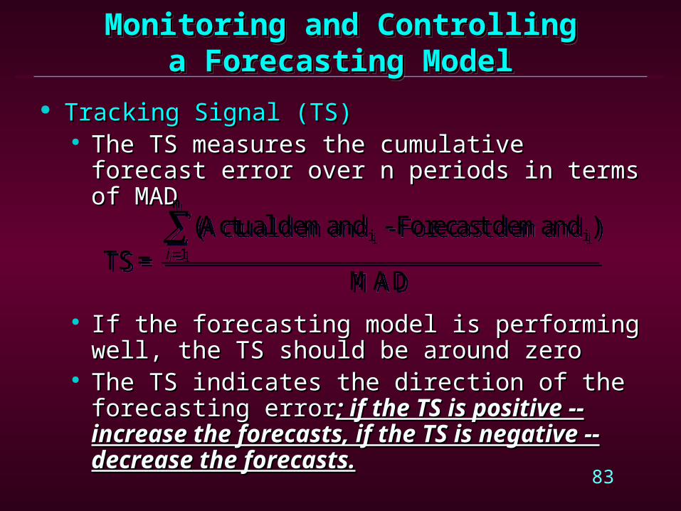
Tracking Signal (TS)Tracking Signal (TS) The TS measures the cumulative forecast error The TS measures the cumulative forecast error

over n periods in terms of MADover n periods in terms of MAD

If the forecasting model is performing well, the TS If the forecasting model is performing well, the TS should be around zeroshould be around zero

The TS indicates the direction of the forecasting The TS indicates the direction of the forecasting errorerror; if the TS is positive -- increase the ; if the TS is positive -- increase the forecasts, if the TS is negative -- decrease the forecasts, if the TS is negative -- decrease the forecasts.forecasts.

n

i i1

(Actual demand - Forecast demand )TS =

MADin

i i1

(Actual demand - Forecast demand )TS =

MADi

84

Computer Software for ForecastingComputer Software for ForecastingComputer Software for ForecastingComputer Software for Forecasting

Examples of computer software with forecasting Examples of computer software with forecasting capabilitiescapabilities Forecast ProForecast Pro AutoboxAutobox SmartForecasts for WindowsSmartForecasts for Windows SASSAS SPSSSPSS SAPSAP POM Software LibaryPOM Software Libary

Primarily forPrimarily forforecastingforecasting

HaveHaveForecastingForecasting

modulesmodules

1 Chapter 3 Demand Forecasting. 2 OverviewOverview l Introduction l Qualitative Forecasting Methods...

Documents

Transcript of 1 Chapter 3 Demand Forecasting. 2 OverviewOverview l Introduction l Qualitative Forecasting Methods...