1 CHAPTER 2 Graph Foundations of Network Modelling M. Pickavet and C. Develder.

1

CHAPTER 2 Graph Foundations of Network Modelling

M. Pickavet and C. Develder

Graph foundations of

network modelling 2

0. Introduction1. Definition and notations

1.1 Graph1.2 Digraph

2. Minimum spanning tree problem 3. Shortest path problem

3.1 in unweighted (di)graphs3.2 in weighted (di)graphs (positive weights)3.3 in weighted (di)graphs (general weights)3.4 all-pairs shortest path

Outline


network modelling 3

4. Maximum flow problem4.1 Network flow4.2 Problem definition4.3 Residual network concept4.4 Flow augmenting path algorithm4.5 Max-flow min-cut theorem4.6 Application: calculation of connectivity

5. Minimum cost flow problem5.1 Introduction5.2 Problem definition5.3 Residual network5.4 Busacker-Gowen algorithm5.5 Several supply/demand vertices

6. Extension: multi-commodity flow problems

Outline


network modelling 4

0.Introduction1. Definition and notations2. Minimum spanning tree problem3. Shortest path problem4. Maximum flow problem5. Minimum cost flow problem6. Extension: multi-commodity flow

problems

Outline


network modelling 5

efficient transfer of information across a communication network network flow problem

flow algorithm

Examples :• shortest path problem• maximum flow problem• minimum cost flow problem

Why graph foundations in a MM network course?


network modelling 6

What must be modeled ?

all the relevant data of the real network:

• topology

• transfer of information

• different parameters

• cost of equipment

• capacity of equipment

• …

Abstract modelling of communication networks


network modelling 7



2. Minimum spanning tree problem3. Shortest path problem4. Maximum flow problem5. Minimum cost flow problem6. Extension: multi-commodity flow

problems

Outline


network modelling 8

e4

e1

e3

e2

e5

• edge set E

==> {e1, e2, e4}

v1 v2

v3v4

• vertex set V

G =(V, E)• graph order p = #V = 4

• graph size q = #E = 5

• G is a (p, q) - graph

• e = uv• incidence: I (v1) = {e1,e2,e3}

• adjacency: A(v2) = {v1,v3}

• degree: (v3) = 3

NODEIP router,

SDH cross-connect,ATM switch,

telephone switch,...

LINKSTM-N,

optical fiber, ...

Subgraph G[W] : subset W of vertices of G + edges incident to vertices of subgraph W only

example : {v1, v2, v3}

Terminology and notations

Graph foundations of network modelling 10

v1 v2

v3v4

e4

e1

e3

e2

e5

walk w = (v0, v1, …, vn-1, vn) such that for i = 0, 1, …, n-1, vivi+1 E

(v1, v4, v3) is a path with length 2Walk with all vertices distinct

(v1, v4, v3, v1) is a cycle with length 3Walk with all vertices but

the first and the last distinct

Special types of walks : paths / cycles

Paths and Cycles


v1 v2

v3v4

e4

e1

e3

e2

e5

v5

e6

e7

e8

G is connected : vertex pairs {u, v}, a path exists between u and v

• cut, e.g. {e2, e3, e5}

• cutset (= minimal cut), e.g. {e3, e5}

• vertex-cut, e.g. {v1, v2, v3}

• vertex-cutset (= minimal vertex-cut), e.g. {v1, v3}

Cut and Cutset


A graph G with edge-connectivity(G) = 2(= minimum cardinality cutset = # {e3,e5})and vertex-connectivity (G) = 2(= minimum cardinality vertex-cutset = # {v1,v3})

v1 v2

v3v4

e4

e1

e3

e2

e5

v5

e6

e7

e8

A graph G with bridge e6

(note that v5 is not a cutvertex)(G) = 1, (G) = 1

v1 v2

v3v4

e4

e1

e3

e2

e5

v5

e6

Connectivity


EXERCISE

edge-connectivity(G) = ?vertex-connectivity (G) = ?

v1v2

v3

v4

v5v6

v7v8

Connectivity




2. Minimum spanning tree problem3. Shortest path problem4. Maximum flow problem5. Minimum cost flow problem6. Extension: multi-commodity flow

problems

Outline


D = (V,A)

• digraph order = #V = 4

• digraph size = #A = 5

Directed Graph

a4

a1

a3

a2

a5

v1 v2

v3v4

• vertex set V

• arc set A

• from - incidence : I (v1) = {a1, a3}

• to - incidence : I’(v4) = {a3, a5}

• from - adjacency : A(v3) = {v1,v4}

• to - adjacency : A’(v2) = {v1}

• out - degree : (v3) = 2

• in - degree : ’(v1) = 1

Digraph


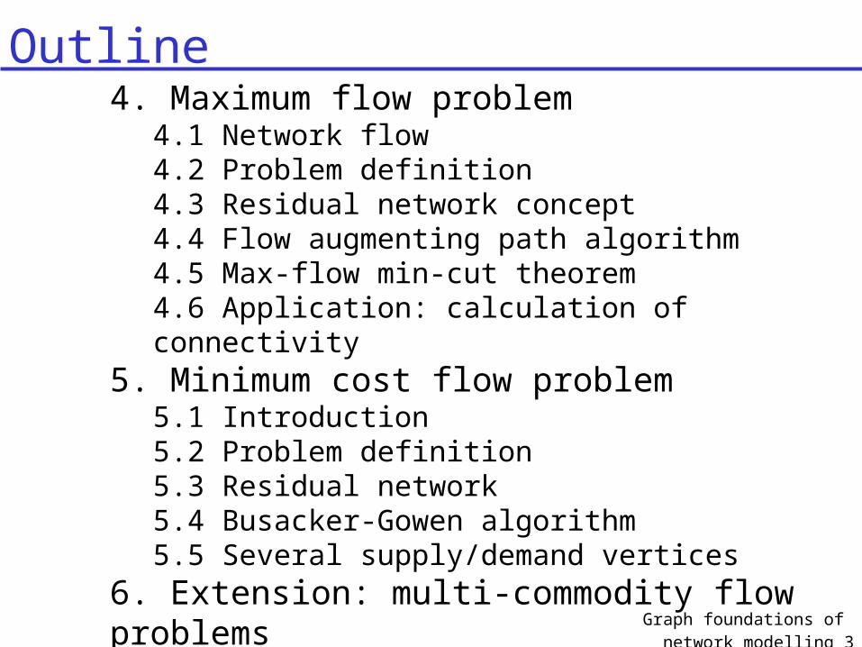
walk w = (v0, v1, …, vn-1, vn) such that for i = 0, 1, …, n-1, (vi,vi+1) A

semiwalk = (v0, v1, …, vn-1, vn) such that for i = 0, 1, …, n-1, (vi,vi+1) A (vi+1,vi A

(v1, v2, v3) is a path with length 2

(v1, v2, v3, v1) is a cycle with length 3

(v1, v4, v3) is a semipath with length 2

(v1, v4, v3, v1) is a semicycle with length 3

a4

a1

a3

a2

a5

v1 v2

v3v4

Paths and Cycles


v1 v2

v3v4

v5

this digraph is strongly connected (u,v)- AND (v,u)-paths

v1 v2

v3v4

v5

this digraph is weakly connected (u,v)- AND/OR (v,u)-paththere are no paths terminating in v3

Strong and weak connectedness


0. Introduction1. Definition and notations2. Minimum spanning tree problem3. Shortest path problem4. Maximum flow problem5. Minimum cost flow problem6. Extension: multi-commodity flow

problems

Outline


v1 v2

v3v4

v5

a tree T=(V,F)• T is connected• T does not contain cycles T contains #V-1 edges

a spanning tree T=(V,F) of G• T is a tree• T has the same vertex set as G

v1 v2

v3v4

v5

Tree and spanning tree


16

2

3

5

4105

170

140

245

139

137180

306

85300

112270

135

206210

Sagninaw

Mackinaw City

Traverse City

Benton Harbor Detroit

GrandRapids

weighted graphc(e) = weight of edge eweight of weighted graph = sum of weights of all edgesminimum spanning tree = spanning tree with minimum weight (in a weighted graph)

{insertion of edge 45 with weight 140 into F} P = { {1,2,3,4,5,6} }

P = { {1}, {2}, {3}, {4}, {5}, {6} }

{insertion of edge 56 with weight 85 into F} P = { {1}, {2}, {3}, {4}, {5,6} }

{insertion of edge 34 with weight 105 into F} P = { {1}, {2}, {3,4}, {5,6} }

{insertion of edge 12 with weight 112 into F} P = { {1,2}, {3,4}, {5,6} }

{insertion of edge 25 with weight 135 into F} P = { {1,2,5,6}, {3,4} }

MST: algorithm of Kruskal


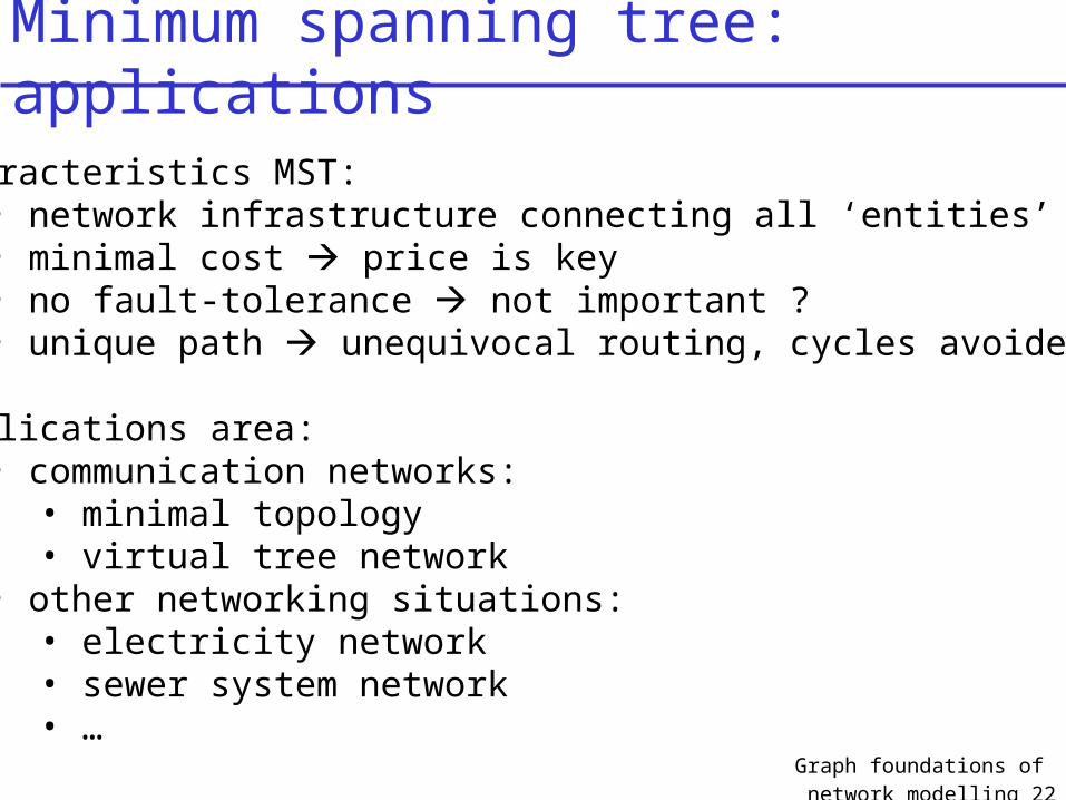
Characteristics MST:• network infrastructure connecting all ‘entities’• minimal cost price is key• no fault-tolerance not important ?• unique path unequivocal routing, cycles avoided

Applications area:• communication networks:

• minimal topology• virtual tree network

• other networking situations:• electricity network• sewer system network• …

Minimum spanning tree: applications


0. Introduction1. Definition and notations2. Minimum spanning tree problem3. Shortest path problem

3.1 In unweighted (di)graphs3.2 In weighted (di)graphs (positive weights) 3.3 In weighted (di)graphs (general weights)3.4 All-pairs shortest path problem

4. Maximum flow problem5. Minimum cost flow problem6. Extension: multi-commodity flow

problems

Outline


The length of a path in an unweighted graph is equal to the number of edges in the path (=‘hopcount’).

The distance d(u,v) between two vertices u,v in a graph G = (V,E)is equal to the length of a shortest u,v-path in G, if such a path exists (if not: d(u,v) = ).

Distance in unweighted graph


v7

3

v3v4 v10v6

2

v1

v4 v6

v9

v10

s

v2 v3

v5v7

v8

G:

0 1 1 1

s v1 v2 v3 v4 v5 v6 v7 v8 v9 v10

0

v8 v9

v2v5v1 1

0 1 1 2 2 1 2 2

0 1 1 2 2 1 2 3 2

s Labels0

Example : the Moore Algorithm





problems

Outline


Weighted Graph : c : E R : map every edge to a real number

Length of a path : sum of length of its edges

Distance between two vertices s,t : length of shortest s,t path

Distance in weighted graph


8

7911

13

14

16

175

µ0=s

v2

v3

v4

v5

v6v7

0 (,-) (,-) (,-) (,-) (,-) (,-) µ0

(25,v5) (15,v5) (,-) (,-) v4

(13,µ0) (,-) (16,µ0) (8,µ0) (,-) (,-) v5

(13,µ0) (25,v5) (15,v5) (,-) (,-) v2

l(µ0) v2 v3 v4 v5 v6 v7 add to

P

(20,v4) (,-) (,-) v3

(,-) (,-)

Assumption :all weights positive !!

shortest path tree

temporal branches

new branches

Algorithm of Dijkstra


EXERCISE

v1v2 v3

v4

v5

v6 v7 v8

u0

1

2

3

4

56

3

3

2

21

5

2

4

1

d(u0,v5) ?1. op zicht2. m.b.v. Dijkstra

Dijkstra


EXERCISE

Dijkstra


Algorithm of Dijkstra: application

[AB,BD,BC]

[BD,CD,DE]

[AE,DE]

[AB,AE]

incominglink statepackets

Router C : Link-State Database

Link Cost From AB 1 A AE 1 A BD 1 B BC 1 B CD 1 D DE 1 D

knowledge ofnetwork topology

Dijkstra : shortest paths

Router C : Routing Table

Dest. Nexthop

Interface

A B BCB Direct BCD Direct CDE D CD

A B

DE

C

LSA E {E-D, E-A}LSA E

{E-D

, E-A

}

LSA E {E-D, E-A}

LS

A E

{E

-D, E

-A}

LSA E {E-D, E-A}

LS

A E

{E

-D, E

-A}





problems

Outline


Principle : label correcting algorithm

v1 v2

v3v4

ts

- 4

31

1

1

2

4

4

1

l(s) = 0

l(t) = 5

l(v2) = 4l(v1) = 3

l(v4) = 1 l(v3) = 2

l(v1) l(v2) + c(v2v1) is violated

l(v1) is updated and set to l(v1) = l(v2) + c(v2v1)

= 0

Let l(i), iV be a set of labels. These labels represent the shortest path distances from the source vertex s if they satisfy the following conditions:

(i) l(s) = 0;(ii) l(i) is the length of some (s,i)-path;(iii) l(j) l(i) + c(ij), (i,j) A

The algorithm of Ford, Bellman and Moore

Result with Dijkstra:


(1) l(s) := 0 ; vV\{s} do l(v) := end;

(2) insert s into List;

(3) while List is not empty do

(4) select the first element v from List and remove it from List;

(5) wA(v) do

(6) if l(w) > l(v) + c(vw)

(7) l(w) := l(v) + c(vw);

(8) if w is not yet an element of List, insert w at the back of List;

(9) end;

(10) end;

l(s)=0, l(v1)=l(v2)=…=l(t)=

List={s}

v=s, List = { }

A(v)={v1,v4}

l(v1)=4, l(v4)=1 List = {v1,v4

}

v=v1, List = {v4 }

A(v)={v4}

A(v)=from-adjacencyin digraph

l(v4)=1

List = {v4 }

v1 v2

v3v4

ts

- 4

31

1

1

2

4

4

1

l(s)=0

Extension : negative cycles ?

The algorithm of Ford, Bellman and Moore


EXERCISE

v1 v2 v3

v4

v5

v6 v7 v8

1

2

3

4

56

3

3

2

-6-1

5

2

u0 4

1

Ford-Bellman-Moore





problems

Outline


All-pairs shortest path problem

v18

711

13

14

16

175

v2

v3

v4

v5

Until now:

• Shortest path from s to t

• Side effect: shortest path tree from s to all other nodes

Current subsection:

Shortest path between ALL PAIRS OF NODES

Possible approaches:

• p times Dijkstra

• Dedicated algorithm: Floyd


Algorithm of Floyd

8

711

13

14

16

175

v1

v2

v3

v4

v5

0 13 16 8

13 0 14 11

14 0 5 17

16 5 0 7

8 11 17 7 0

v1 v2 v3 v4 v5

v1

v2

v3

v4

v5

Step 0: direct paths distances

0 13 16 8

13 0 14 29 11

14 0 5 17

16 29 5 0 7

8 11 17 7 0

v1 v2 v3 v4 v5

v1

v2

v3

v4

v5

Step 1: x – v1 – y better ?

0 13 27 16 8

13 0 14 29 11

27 14 0 5 17

16 29 5 0 7

8 11 17 7 0

v1 v2 v3 v4 v5

v1

v2

v3

v4

v5

Step 2: x – v2 – y better ?

?

Assumption :all weights positive !!


Algorithm of Floyd

8

711

13

14

16

175

v1

v2

v3

v4

v5

0 13 27 16 8

13 0 14 19 11

27 14 0 5 17

16 19 5 0 7

8 11 17 7 0

v1 v2 v3 v4 v5

v1

v2

v3

v4

v5

Step 3: x – v3 – y better ? Step 4: x – v4 – y better ?

v1 v2 v3 v4 v5

v1

v2

v3

v4

v5

0 13 21 16 8

13 0 14 19 11

21 14 0 5 12

16 19 5 0 7

8 11 12 7 0

Step 5: x – v5 – y better ?v1 v2 v3 v4 v5

v1

v2

v3

v4

v5

0 13 20 15 8

13 0 14 18 11

20 14 0 5 12

15 18 5 0 7

8 11 12 7 0


Algorithm of Floyd

(1) D(0) = A;

(2) for step := 1 to p do

(3) for vi := v1 to vp do

(4) for vj := v1 to vp do

(5) di,j(step) := min {di,j

(step-1) , di,vstep(step-1) + dvstep,j

(step-1) }

(6) end;

(7) end;

(8) end.

8

711

13

14

16

175

v1

v2

v3

v4

v5Implementation effort: small

Time complexity: O(p3)

p times Dijkstra: p x O(p2)


0. Introduction1. Definition and notations2. Minimum spanning tree problem3. Shortest path problem4. Maximum flow problem

4.1 Network flow4.2 Problem definition4.3 Residual network concept4.4 Flow augmenting path algorithm4.5 Max-flow min-cut theorem4.6 Application: calculation of connectivity

5. Minimum cost flow problem6. Extension: multi-commodity flow

problems

Outline


abstract modelling of a communication network

transfer of information flow

topology directed graph (digraph) D = (V,A)

every arc a A has associated numerical values cost c(a) weighted digraph

capacity u(a) capacitated digraph

network N = weighted, capacitated digraph (V,A)

Network flow models


(2) ,)()(0

(1) v,v)()()v(')v(

Aaauaf

VbafafIaIa

flow function f (.) : A Z+ or R+

subject to the following constraints:

u(a) = capacity of link

capacityconstraints

•supply vertex : b(v) > 0 (source)•demand vertex : b(v) < 0 (sink)

flow conservation

v I(v)I’(v)

Network flow-associated constraints





problems

Outline


Aaauaf

tvF

tsVv

svF

afaf

F

vIa vIa

,)( )( 0

if,

},{\,0

if,

)()(

subject to

maximize

)( )('

t

v3

sSource Sink

v1

v4

v22

3

45

3

3

i jcapacity

u(ij)1 1 1

Problem definition : maximum flow





problems

Outline


[0,2]

[0,4]

[0,3]

[0,1]

[0,5]

i j[ f °(ij),u(ij)]

i jr(ij)

original network

Source Sink1 4

3

2

1

1

1

2

2

35

1 4

3

2

residual network

flow capacity

[0,2]

[3,4]

[0,3]

[0,1]

[3,5]

[2,2]

[3,4]

[2,3]

[0,1]

[5,5]

flow=3flow=2

residual capacity

Residual network concept


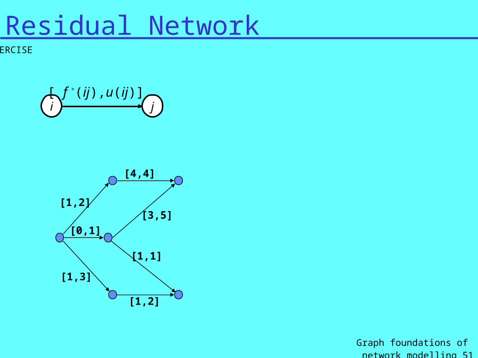
EXERCISE

[0,1]

[1,2]

[4,4]

[3,5]

[1,3]

[1,2]

[1,1]

i j[ f °(ij),u(ij)]

Residual Network





problems

Outline


1

1

2

2

2

24

1 4

3

2

1

source sink

residual network N(f) :

(1) f := 0; (2) while ( N (f ) contains at least one augmenting path from s to t ) do (3) identify one augmenting path P from vertex s to vertex t; (4) d := min{r(ij) : ij P}; (5) augment the flow f with d units along P; (6) update N (f ); (7) od

determine the maximum flow between two vertices s and t in a network N.

augmenting path ?

d = residual capacityof augmenting path

1

Flow Augmenting Path Algorithm


1

2

3

4Source Sink

4

2 1

5

(a)

3 1

2

3

4

(b)

1

2

3

4

1

4

1

2

3

4

(c)

111

2 1

4 5

1

2

3

4

(d)

4 5

2

2

1

1

r(ij)i j

Flow Augmenting Path Algorithm


4

3 5

6

2

i j

1

r(ij)

2

2

2

2

2

2

2

(c)

r(ij)i j

2 4

5

1

3

6

2

2

2

2

2

2

2

(b)

4

6

5

1

i j

2

3

[f (ij), u(ij)]

[0,2]

[2,2]

[2,2]

[2,2]

[2,2]

[2,2]

[2,2]

(d)

i j

6

5

1Source Sink

2

[ f (ij), u(ij)]

3

4[0,2]

[2,2]

[2,2]

[2,2]

(a)

[0,2]

[0,2]

[0,2]

?

Orig.

Orig.

Res.

Res.

Do we need a residual network ??


EXERCISE

i jcapacity

u(ij)

A

B

5

2

21

2

2

7

1

22 3

1

55

55

2

capi j

Maximum Flow Algorithm


Maximum Flow Algorithm: applications

Characteristics max. flow solution:• from one source to one destination• maximal use of network BW

bifurcation of flow compliant with application ? (different delays, reordering, …)

• cost of paths not taken into account

Some applications:• maximum BW from server client• indication on available BW source destination• restoration mechanism: available spare capacity ?


Maximum Flow Algorithm: applications

via spare capacityin network





problems

Outline


correspondence between flows and cuts in a network

minimum cut problem : “From among all cuts in the network

that separate the source and the sink, find the cut with minimum capacity”.

i ju(ij)

t

v3

sSource Sink

v1

v4

v22

2

4 4

3

3

1 1 1

Network example:

st : 8st : 6

The Maximum-Flow Minimum-Cut Theorem


Example: maximum s,t-flow F = 6

i jf(ij)

t

v3

sSource Sink

v1

v4

v22

2

34

3

3

1 1 1

The maximum value of a flow between s and t =

capacity of a minimum s,t-cut

Theorem:

minimum-cut

The Maximum-Flow Minimum-Cut Theorem





problems

Outline


Max flow min cut theorem :(v,w)

(v,w) = minimum cardinality of a v,w-edge-cutset

(G) = edge-connectivity of graph G = min{(v,w) | v,w V }.

(v,w) = 3

Graph G

v w

y

x

How to calculate (v,w) ?

ResidualNetwork :

v w

111

11

11

1

1

1

1

1

11

11

(x,y) = 2 (G) = 2

= maximum flow F(v,w) (if all link capacities = 1)

(v,w) = max. # edge-disjoint paths between v

and w

Calculation of edge-connectivity


v w

111

11

11

1

1

1

1

1

11

11

v w

12

222

1

1

1

11

11

v w

222

2

2

1

1

2

11

v w

222

2

2

2

2

2

3 edge-disjoint paths (v,w)=3

Calculation of edge-connectivity


v’ v”= s t = w’ w”

x’ x”

y’ y”

1

1 1 1 1 1

1

1

1

l

l

ll

(v,w) = minimum cardinality of a v,w-vertex-cutset (v,w non adjacent)(G)=min{(v,w) | v,wV, vw E}

v w

x

y

(v,w) = 2(G) = 2

Graph G(v,w) = max. # vertex-disjoint paths between v and w

How to calculate (v,w)

• Split vertices : v’, v”• Interconnect vertices : v’v”, v’w”, v”w’ (all link capacities = 1)

• (v,w) = maximum flow F(v”,w’)

Calculation of vertex-connectivity


v’ v” w’ w”

x’ x”

y’ y”

1

1 1 1 1 1

1

1

1

l

l

ll

(v,w) = 2

Calculation of vertex-connectivity


Connectivity: applications

Network survivability:• to cope with single link failures: edge-connectivity 2• to cope with single node failures: vertex-connectivity 2• to cope with two links failing simultaneously: edge-connectivity 3• …


0. Introduction1. Definition and notations2. Minimum spanning tree problem3. Shortest path problem4. Maximum flow problem5. Minimum cost flow problem

5.1 Introduction5.2 Problem definition5.3 Residual network5.4 Busacker-Gowen algorithm5.5 Several supply/demand vertices


Outline


i j[c (ij),u (ij)]

t

v3

sServer Source Sink Client

v1

v4

v2[5,2]

[2,3]

[1,4][3,5]

[2,3]

[3,3]

[1,1] [1,1] [1,1]

Example:

demand (sourcesink) = 6

Minimize the total cost of flowwith respect to how to route the flow

subject to• the flow value on each arc respects the arc capacity• the total flow fulfills the demand between s and t

Introduction





Outline


Optimisation model for minimum cost flow problem

minimize

subject to

if

if

c a f a

f a f a

d v s

v V s t

d v t

f a u a a A

a A

a I v a I v

( ) ( )

( ) ( )

,

, \ { , }

,

( ) ( ),

( ) ' ( )

0

0

Problem definition





Outline


Residual network concept

original network Nwith a certain flow f °(ij)

correspondingresidual network N( f °)

i jc(ij),u(ij),f(ij)

i j

[c(ij), r(ij) = u(ij) - f °(ij)]

[-c(ij), r(ji) = f °(ij)]

every arc (i,j) in original network two arcs (i,j) and (j,i) in residual network


Residual network : example

i j[c(ij),r(ij)]

(a)

original network Nwith a certain flow f °

correspondingresidual network N( f °)

[c(ij),u(ij)]i j

f °(ij)

[1,1][-1,2]

[-2,2]

1 4

3

2

[3,2]

[4,4] [1,2]

[-1,2]

Source Sink1 4

3

2

[2,2]

[4,4]

[1,3]

[3,2]

[1,4]

2

2

2

(b)





Outline


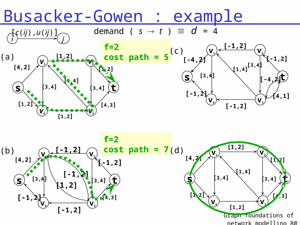
algorithm to determine a minimum cost flow f in a network N from a source vertex s to a sink vertex t with value d (demand).

(1) f ; // initially there is no flow in the network

(2) while ( F < d ) do (3) identify the shortest augmenting path P from s to t in N( f ); (4) min { min{ r(ij) : ij P }, (d F ) } ;

(5) augment the flow f along P with ; (6) update N ( f ); (7) F F ; (8) od

Remarks : (i) It is assumed that a feasible flow from s to t with value d is possible.

(ii) Flow value F f aa I s

( )( )

The algorithm of Busacker and Gowen


Busacker-Gowen : exampledemand ( s t ) d = 4

i j[c(ij),u(ij)]

t

v3

s

v1

v4

v2

[1,2]

[1,2]

[1,2][4,2]

[1,2]

[4,3]

[3,4][1,4]

[3,4]

t

v3

s

v1

v4

v2

[4,2]

[4,3]

[3,4] [3,4]

[-1,2]

[-1,2]

[-1,2]

[-1,2]

[-1,2]

[1,2]

f=2cost path = 5

t

v3

s

v1

v4

v2

[1,2]

[1,2]

[1,2][4,2]

[1,2]

[4,3]

[3,4][1,4]

[3,4]

f=2cost path = 7

t

v3

s

v1

v4

v2

[-1,2]

[-1,2]

[-1,2][-4,2]

[-1,2]

[-4,2][3,4]

[3,4][1,4]

[4,1]

(a)

(b)

(c)

(d)


EXERCISE

t

v3

s

v1

v4

v2

[3,1]

[3,2]

[1,2][2,2]

[3,2]

[2,2]

[3,4][1,4]

[3,4]

d =3

i j[c(ij),u(ij)]

Busacker-Gowen





Outline


minimize

subject to

c a f a

f a f a b v v V

f a u a a A

a A

a I v a I v

( ) ( )

( ) ( ) ( ) ,

( ) ( ) ,( ) '( )

0

Optimisation model :

t

t2

ssuper-supply super-demand

s1

s2

t1[5,2]

[0,2]

[0,4][0,5]

[2,3]

[0,3]

[1,1][1,1]

[1,1]

demand = 5+2 = 4+3 = 7

Min cost flow algorithm :

b(s1) = +5

b(s2) = +2

b(t1) = -4

b(t2) = -3

i j[c(ij),u(ij)]

t2

s1

s2

t1[5,2]

[2,3]

[1,1][1,1]

[1,1]

Example :Several supply/demand vertices


0. Introduction1. Definition and notations2. Minimum spanning tree problem3. Shortest path problem4. Maximum flow problem5. Minimum cost flow problem6. Extension: multi-commodity flow 6. Extension: multi-commodity flow

problemsproblems

Outline


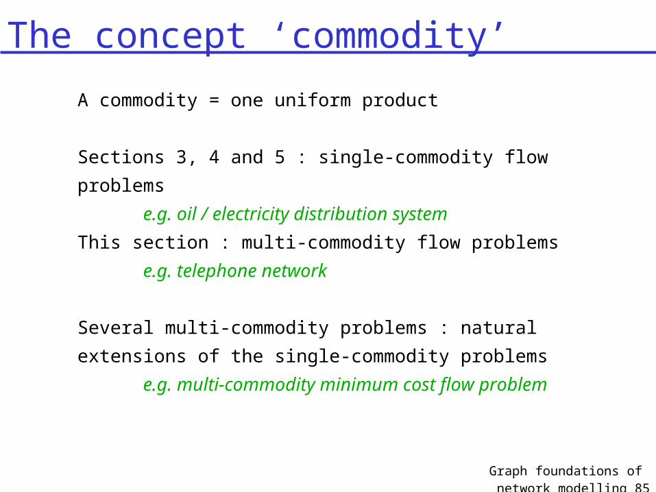
A commodity = one uniform product

Sections 3, 4 and 5 : single-commodity flow problems

e.g. oil / electricity distribution system

This section : multi-commodity flow problems

e.g. telephone network

Several multi-commodity problems : natural extensions

of the single-commodity problems

e.g. multi-commodity minimum cost flow

problem

The concept ‘commodity’


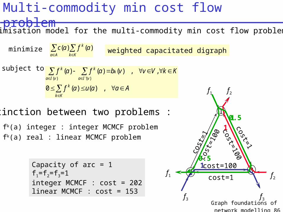
Optimisation model for the multi-commodity min cost flow problem :

subject to f a f a b v v V k K

f a u a a A

k

a I v

k

a I v

k

k

k K

( ) '( )

( ) ( ) ( ) , ,

( ) ( ) ,0

Distinction between two problems :

• fk(a) integer : integer MCMCF problem• fk(a) real : linear MCMCF problem

1

2 3

f1 f2

f1 f2

f3f3

cost=1

cost=100

cost

=100

cost=100cost=1

cost

=1

minimize c a f ak

k Ka A

( ) ( ) weighted capacitated digraph

Capacity of arc = 1f1=f2=f3=1integer MCMCF : cost = 202linear MCMCF : cost = 153

11

1

0.5

0.5

Multi-commodity min cost flow problem


Application: IP routing vs. MPLS Traffic Eng.

very refined granularity (one IP packet = some bytes typical arc capacity = 100s Mbit/s)flow variable has an almost continuous nature real fk(a) variables allowed

Problem: demands for traffic between every pair of IP(/MPLS) routers

IP:only shortest paths allowed algorithm of Dijkstra

IP/MPLS:explicit routes possible (‘traffic engineering’)mathematical formulation: multi-commodity flow problem

A B

DE

CA B

DE

C


Limitations of graph algorithms

Example of multi-commodity flow problems:• distinction between real and integer problem arises• no efficient graph algorithms as solution method

More in general:• graph algorithms for ‘easy’ problems• or parts of ‘difficult’ problems (e.g. network design)

next chapter:• general optimisation techniques • real vs. integer


[1] N. Christofedes: Graph Theory: an Algorithmic Approach (Academic Press, New York, 1975).

[2] G. Chartrand, O. Oellermann: Applied and Algorithmic Graph Theory (McGraw-Hill, New York, 1993).

[3] R.K.Ahuja, T.L.Magnanti, J.B.Orlin, Network Flows (Prentice-Hall, New Jersey, 1993).

[4] M.O.Ball, T.L.Magnanti, C.L.Monma, G.L.Nemhauser, Handbooks in Operations Research and Management Science, vol. 7, Network Models (North-Holland, Amsterdam, 1995).

References

1 CHAPTER 2 Graph Foundations of Network Modelling M. Pickavet and C. Develder.

Documents

Transcript of 1 CHAPTER 2 Graph Foundations of Network Modelling M. Pickavet and C. Develder.