1 Chapter 2 and 3 Forecasting Advanced Forecasting Operations Analysis Using MS Excel.

1

Chapter 2 and 3Chapter 2 and 3

ForecastingForecasting

Advanced ForecastingAdvanced Forecasting

Operations Analysis Using MS Excel

2

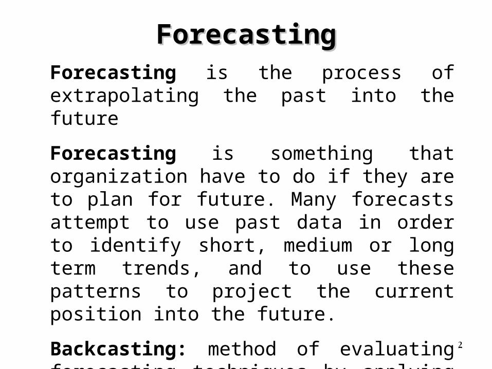
Forecasting is the process of extrapolating the past into the future

Forecasting is something that organization have to do if they are to plan for future. Many forecasts attempt to use past data in order to identify short, medium or long term trends, and to use these patterns to project the current position into the future.

Backcasting: method of evaluating forecasting techniques by applying them to historical data and comparing the forecast to the actual data.

ForecastingForecasting

3

0

1

2

3

4

5

6

7

Jan Feb Mar Apr May Jun Jul Aug Sep Oct Nov Dec Jan

Devia

tio

ns

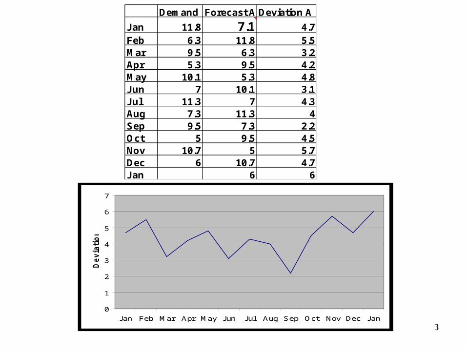
Demand Forecast A Deviation A

Jan 11.8 7.1 4.7Feb 6.3 11.8 5.5Mar 9.5 6.3 3.2Apr 5.3 9.5 4.2May 10.1 5.3 4.8Jun 7 10.1 3.1Jul 11.3 7 4.3Aug 7.3 11.3 4Sep 9.5 7.3 2.2Oct 5 9.5 4.5Nov 10.7 5 5.7Dec 6 10.7 4.7Jan 6 6

4

Forecasting

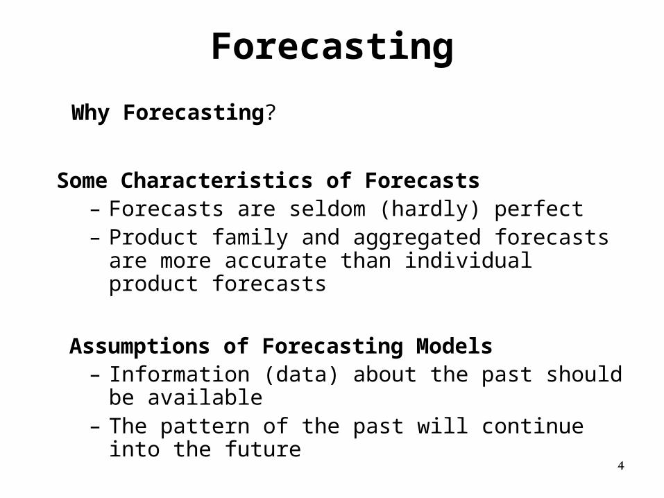
Why Forecasting?

Some Characteristics of Forecasts– Forecasts are seldom (hardly) perfect– Product family and aggregated forecasts are more

accurate than individual product forecasts

Assumptions of Forecasting Models– Information (data) about the past should be available– The pattern of the past will continue into the future

5

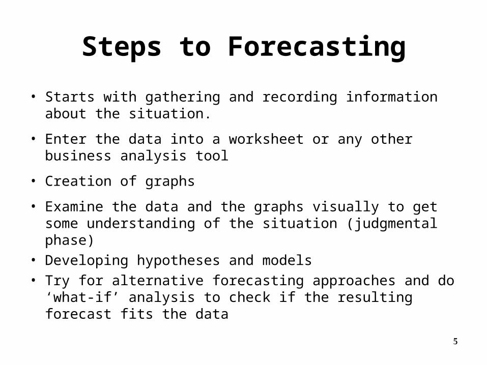
Steps to Forecasting

• Starts with gathering and recording information about the situation.

• Enter the data into a worksheet or any other business analysis tool

• Creation of graphs

• Examine the data and the graphs visually to get some understanding of the situation (judgmental phase)

• Developing hypotheses and models• Try for alternative forecasting approaches and do ‘what-

if’ analysis to check if the resulting forecast fits the data

6

Evaluation of Forecasting ModelEvaluation of Forecasting Model

To judge how well a forecasting model fit the past observation, both precision and bias must be considered.

Measuring the precision of a forecasting model:

There are three possible measures used to evaluate precision of forecasting systems, each of them is based on the error or deviation between the forecasted and actual values: MAD, MSE, MAPE

7

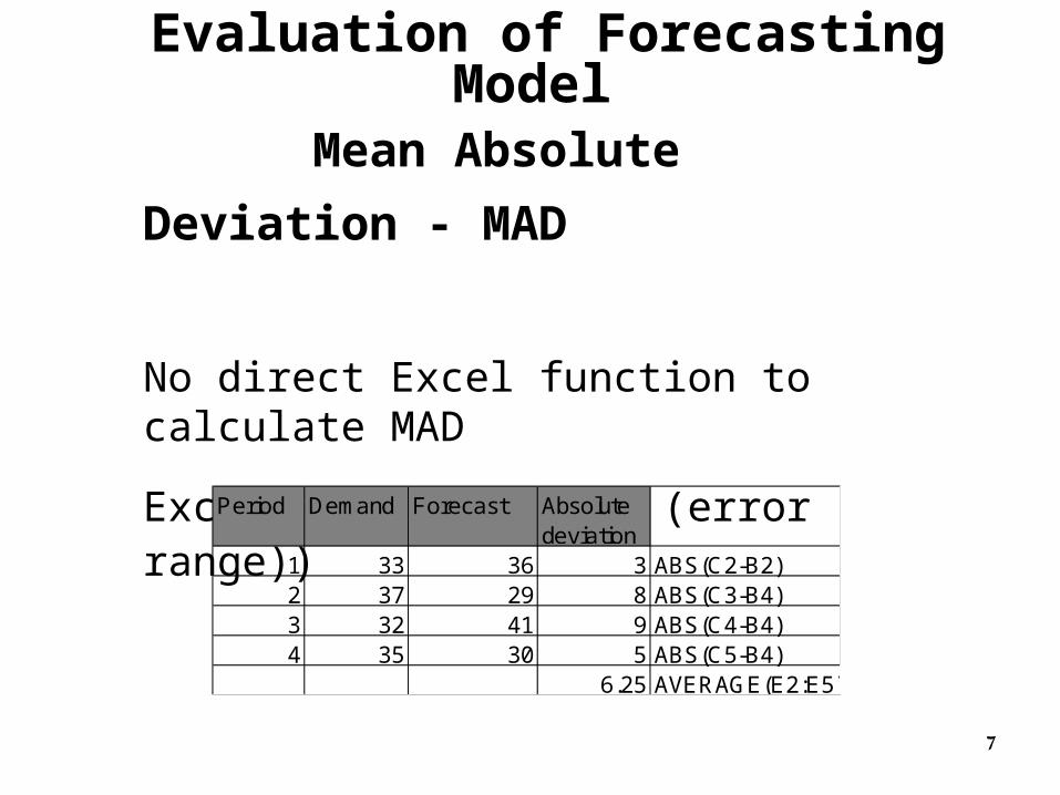
Mean Absolute Deviation - MAD

No direct Excel function to calculate MAD

Excel: =ABS(AVERAGE (error range))

Period Demand Forecast Absolute deviation

1 33 36 3 ABS(C2-B2)2 37 29 8 ABS(C3-B4)3 32 41 9 ABS(C4-B4)4 35 30 5 ABS(C5-B4)

6.25 AVERAGE(E2:E5)

Evaluation of Forecasting Model

8

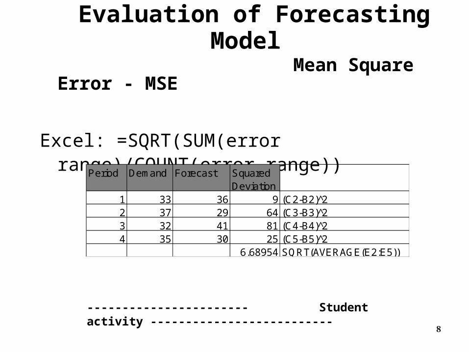
Mean Square Error - MSE

Excel: =SQRT(SUM(error range)/COUNT(error range))

Evaluation of Forecasting Model

Period Demand Forecast Squared Deviation

1 33 36 9 (C2-B2) 2̂2 37 29 64 (C3-B3) 2̂3 32 41 81 (C4-B4) 2̂4 35 30 25 (C5-B5) 2̂

6.68954 SQRT(AVERAGE(E2:E5))

----------------------- Student activity --------------------------

9

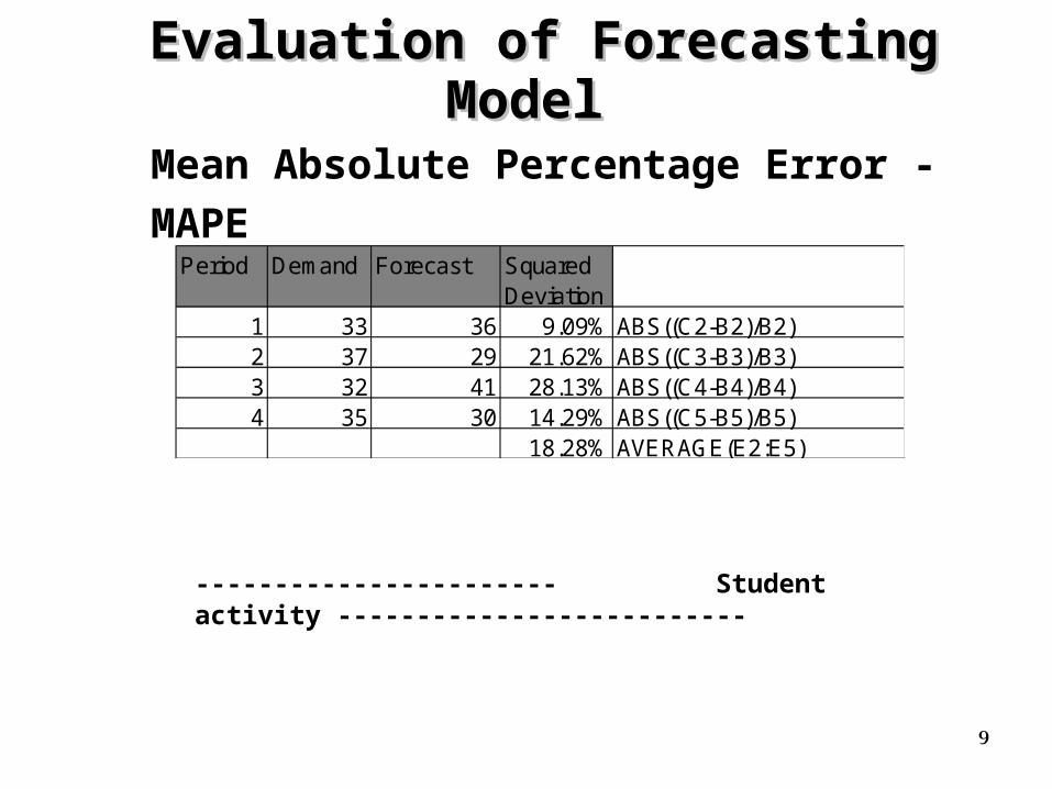
Mean Absolute Percentage Error - MAPE

Evaluation of Forecasting ModelEvaluation of Forecasting Model

Period Demand Forecast Squared Deviation

1 33 36 9.09% ABS((C2-B2)/B2)2 37 29 21.62% ABS((C3-B3)/B3)3 32 41 28.13% ABS((C4-B4)/B4)4 35 30 14.29% ABS((C5-B5)/B5)

18.28% AVERAGE(E2:E5)


10

Which of the measure of forecast Which of the measure of forecast accuracy should be used?accuracy should be used?

The most popular measures are MAD and MSE.

The problem with the MAD is that it varies according to how big the number are.

MSE is preferred because it is supported by theory, and because of its computational efficiency.

MAPE is not often used.

In general, the lower the error measure (BIAS, MAD, MSE) or the higher the R2, the better the forecasting model

11

As it was discussed previously that neither MAD nor MSE gives an accurate indication of the validity of a forecast model. Thus, judgment must be used.

Raw data sample should always be subjected to managerial judgment and analysis before formal quantitative techniques can be applied.

Good Fit – Bad ForecastGood Fit – Bad Forecast

12

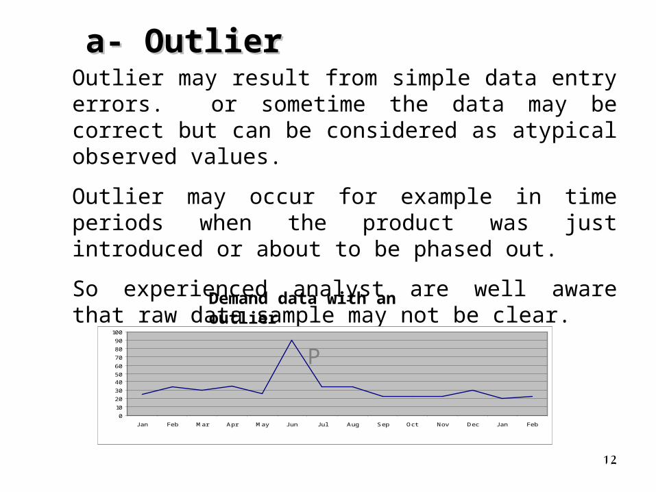
Outlier may result from simple data entry errors. or sometime the data may be correct but can be considered as atypical observed values.

Outlier may occur for example in time periods when the product was just introduced or about to be phased out.

So experienced analyst are well aware that raw data sample may not be clear.

a- Outliera- Outlier

0

10

20

30

4050

60

70

80

90

100

J an Feb Mar Apr May J un J ul Aug Sep Oct Nov Dec J an Feb

P

Demand data with an outlier

13

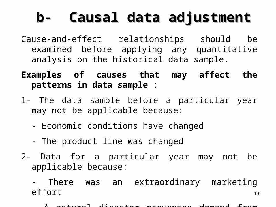
Cause-and-effect relationships should be examined before applying any quantitative analysis on the historical data sample.

Examples of causes that may affect the patterns in data sample :

1- The data sample before a particular year may not be applicable because:

- Economic conditions have changed

- The product line was changed

2- Data for a particular year may not be applicable because:

- There was an extraordinary marketing effort

- A natural disaster prevented demand from occurring

b- Causal data adjustment b- Causal data adjustment

14

The meaning of a “good fit” is subjective to the manager’s interpretation of the forecasting model.

So before a forecast is accepted for action, quantitative techniques must be augmented by such judgmental approaches as decision conferencing and expert consultations.

c- Illusory (misleading) patternsc- Illusory (misleading) patterns

15

- Company actions

- Competitors actions

- Industry demand

- Market share

- Company sales

- Company costs

- Environmental factors

To prepare a valid forecast, the following factors To prepare a valid forecast, the following factors that influence the forecasting model should be that influence the forecasting model should be examined:examined:

16

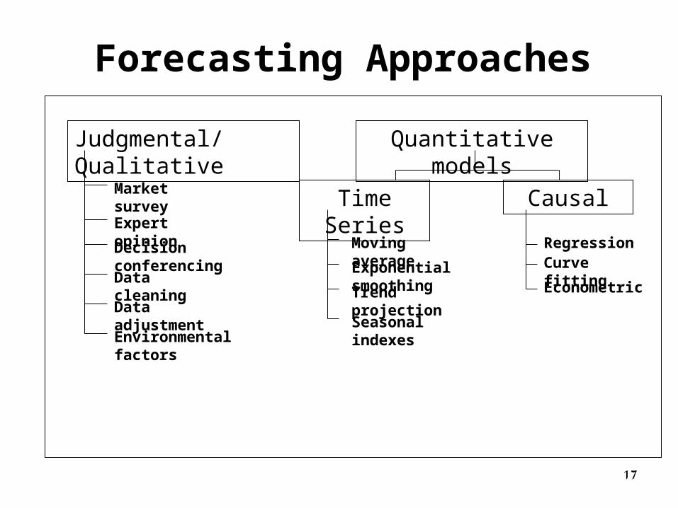
Forecasting ApproachesForecasting Approaches

1-1- Qualitative ForecastingQualitative Forecasting Forecasting based on experience, judgment, and

knowledge. Used when situation is vague and little data exists. Example: new products and new technology

2- 2- Quantitative ForecastingQuantitative ForecastingForecasting based on data and models. Used when situation is ‘stable’ and historical data exist. Example: existing product, current technology

17

Judgmental/Qualitative Quantitative models

Time Series Causal

Moving average

Exponential smoothing

Trend projection

Seasonal indexes

RegressionCurve fitting

Econometric

Market survey

Expert opinion

Decision conferencing

Data cleaning

Data adjustment

Environmental factors

Forecasting Approaches

18

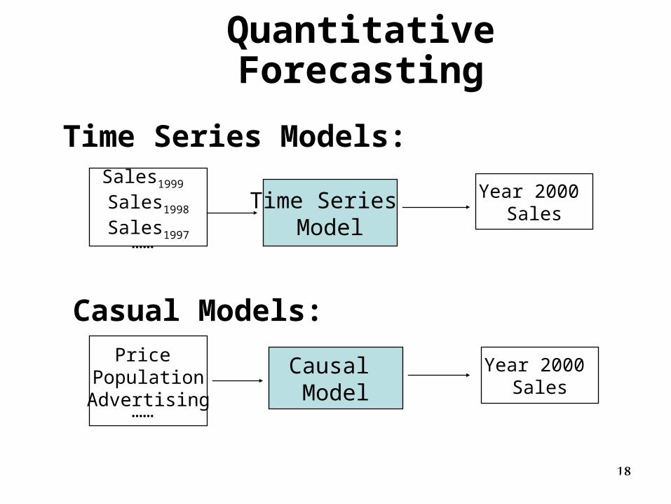
Quantitative Forecasting

Time Series Models:

Time Series Model

Year 2000 Sales

Sales1999 Sales1998

Sales1997……

Casual Models:

Causal Model

Year 2000 Sales

Price PopulationAdvertising

……

19

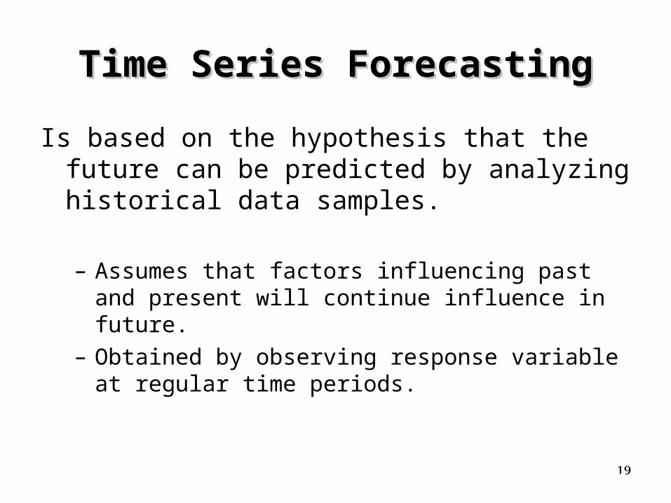
Time Series ForecastingTime Series Forecasting

Is based on the hypothesis that the future can be predicted by analyzing historical data samples.

– Assumes that factors influencing past and present will continue influence in future.

– Obtained by observing response variable at regular time periods.

20

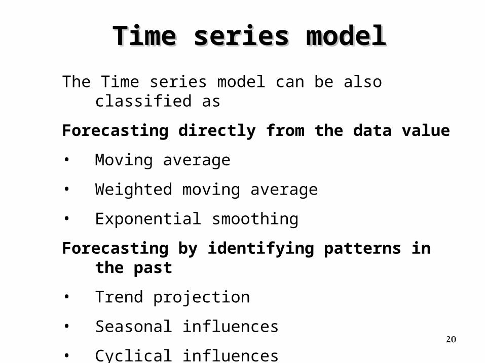
Time series modelTime series model

The Time series model can be also classified as

Forecasting directly from the data value

• Moving average

• Weighted moving average

• Exponential smoothing

Forecasting by identifying patterns in the past

• Trend projection

• Seasonal influences

• Cyclical influences

21

1- Moving Average Method1- Moving Average Method

- The forecast is the mean of the last n observation. The choice of n is up to the manager making the forecast

- If n is too large then the forecast is slow to respond to change

- If n is too small then the forecast will be over-influenced by chance variations

-This approach can be used where a large number of forecasting needed to be made quickly, for example in a stock control system where next week’s demand for every item needs to be forecast

Forecasting directly from the data valueForecasting directly from the data value

22

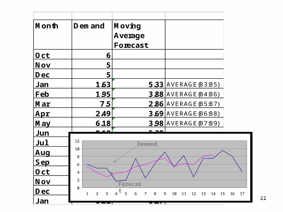
Month Demand Moving Average Forecast

Oct 6Nov 5Dec 5Jan 1.63 5.33 AVERAGE(B3:B5)

Feb 1.95 3.88 AVERAGE(B4:B6)

Mar 7.5 2.86 AVERAGE(B5:B7)

Apr 2.49 3.69 AVERAGE(B6:B8)

May 6.18 3.98 AVERAGE(B7:B9)

Jun 9.18 5.39 =

Jul 5.24 5.95 =

Aug 8.3 6.87 =

Sep 2.72 7.57 =

Oct 7.43 5.42 =

Nov 7.49 6.15 =

Dec 9.58 5.88 =

Jan 8.02 8.17 =

0

2

4

6

8

10

12

1 2 3 4 5 6 7 8 9 10 11 12 13 14 15 16 17

Demand

Forecast

23

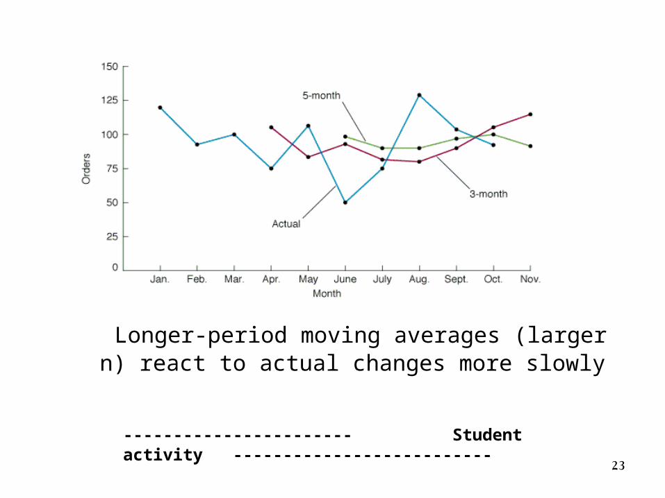
Longer-period moving averages (larger n) react to actual changes more slowly


24

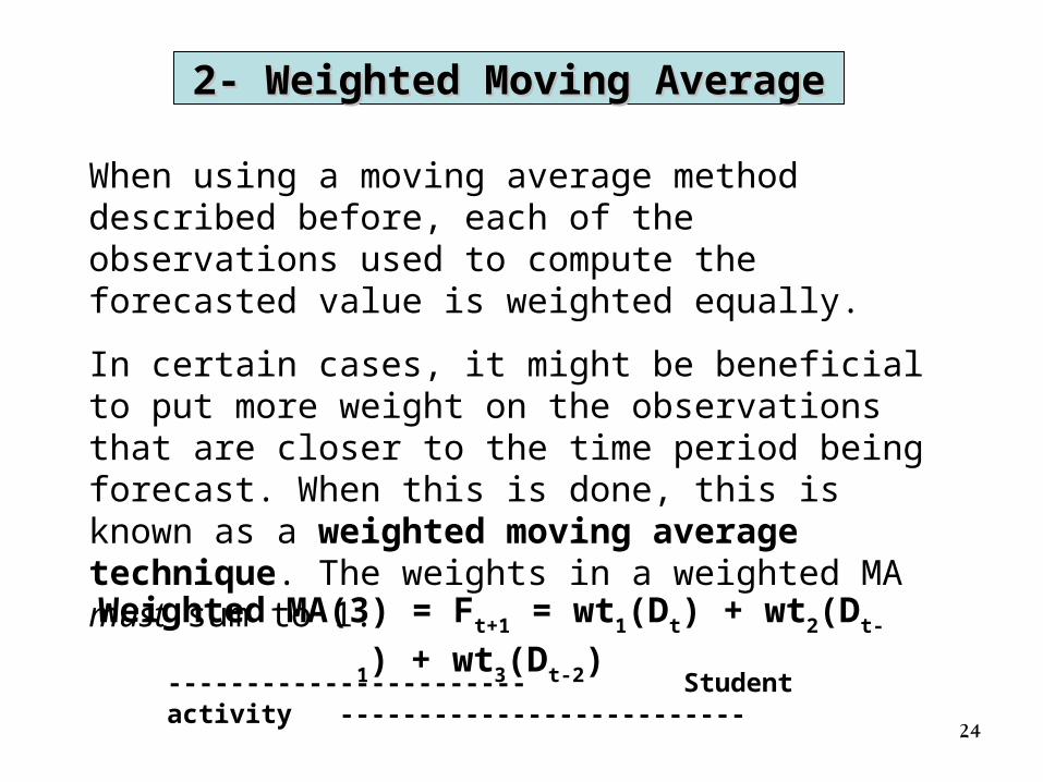
When using a moving average method described before, each of the observations used to compute the forecasted value is weighted equally.

In certain cases, it might be beneficial to put more weight on the observations that are closer to the time period being forecast. When this is done, this is known as a weighted moving average technique. The weights in a weighted MA must sum to 1.

Weighted MA(3) = Ft+1 = wt1(Dt) + wt2(Dt-1) + wt3(Dt-2)

2- Weighted Moving Average2- Weighted Moving Average


25

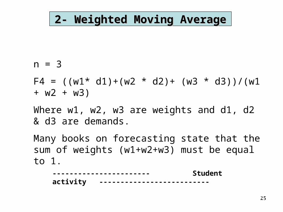
n = 3

F4 = ((w1* d1)+(w2 * d2)+ (w3 * d3))/(w1 + w2 + w3)

Where w1, w2, w3 are weights and d1, d2 & d3 are demands.

Many books on forecasting state that the sum of weights (w1+w2+w3) must be equal to 1.

2- Weighted Moving Average2- Weighted Moving Average


26

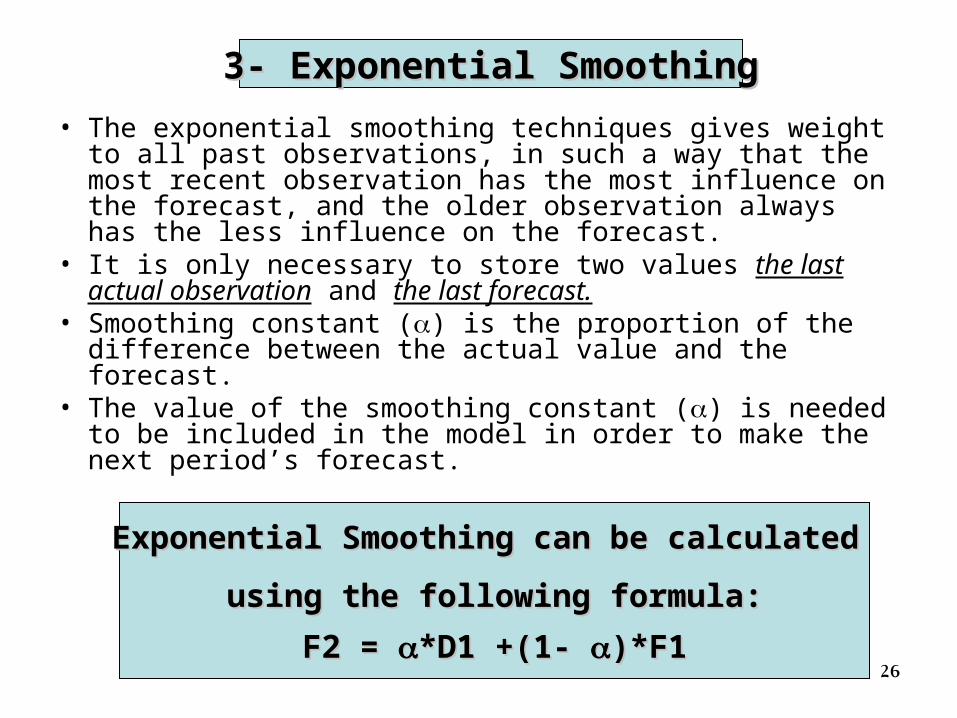
• The exponential smoothing techniques gives weight to all past observations, in such a way that the most recent observation has the most influence on the forecast, and the older observation always has the less influence on the forecast.

• It is only necessary to store two values the last actual observation and the last forecast.

• Smoothing constant () is the proportion of the difference between the actual value and the forecast.

• The value of the smoothing constant () is needed to be included in the model in order to make the next period’s forecast.

3- Exponential Smoothing3- Exponential Smoothing

Exponential Smoothing can be calculated Exponential Smoothing can be calculated

using the following formula:using the following formula:

F2 = F2 = *D1 +(1- *D1 +(1- )*F1)*F1

27

• Smoothing constant () must set between 0 and 1. Normally the value of the smoothing constant is chosen to lie in the range 0.1 to 0.3.

• Typically, a value closer to 0 is used for forecasting demand that is changing slowly, however, value closer to 1 is used for forecasting demand that is changing more rapidly.

• There is no way to calculate F1 because each forecast is based on the previous forecasts.


28

How to select smoothing constant

• Sensitivity analysis is an analysis used to test how sensitive the the forecast is to the change in alpha or smoothing constant.

• A general rule for selecting alpha is to perform scenario analysis and pick the value that produces a reasonable value for the MAD and a forecast that is reasonably close to the actual demand.


29

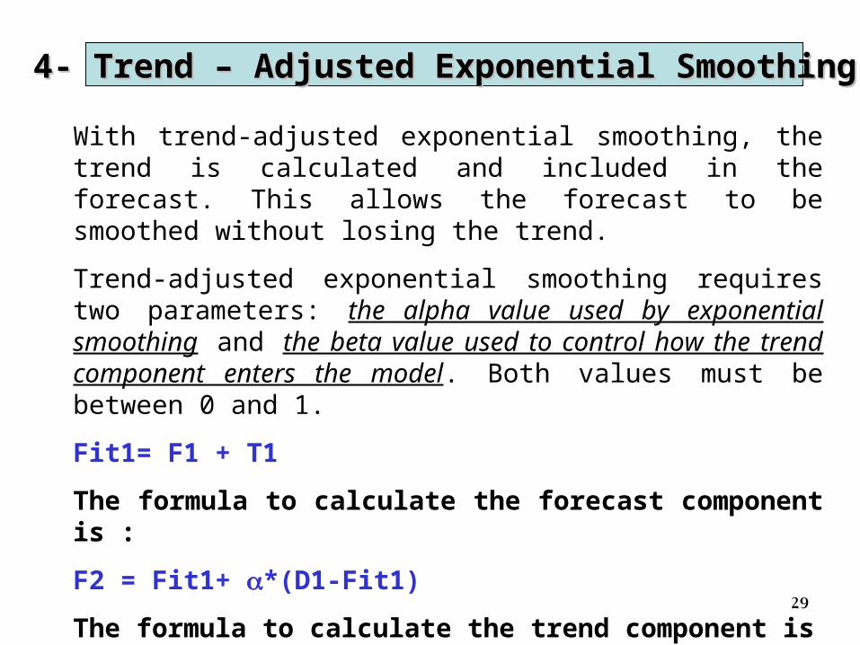
With trend-adjusted exponential smoothing, the trend is calculated and included in the forecast. This allows the forecast to be smoothed without losing the trend.

Trend-adjusted exponential smoothing requires two parameters: the alpha value used by exponential smoothing and the beta value used to control how the trend component enters the model. Both values must be between 0 and 1.

Fit1= F1 + T1

The formula to calculate the forecast component is :

F2 = Fit1+ *(D1-Fit1)

The formula to calculate the trend component is

T2 = T1 + * *(D1-Fit1)

4- Trend – Adjusted Exponential Smoothing4- Trend – Adjusted Exponential Smoothing

30

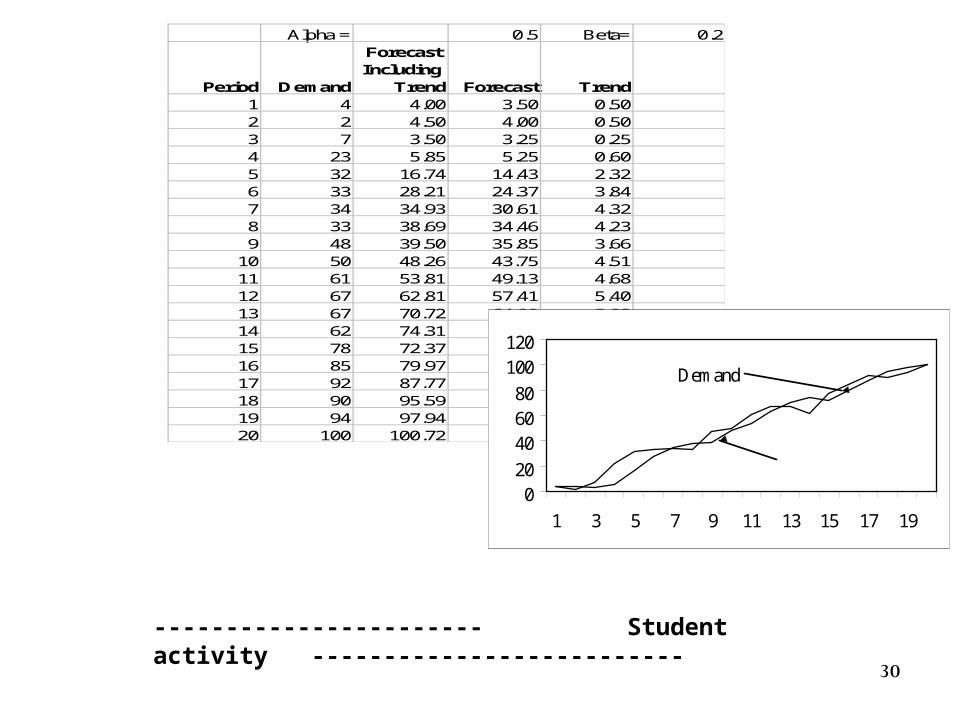
Alpha = 0.5 Beta= 0.2

Period Demand

Forecast Including

Trend Forecast Trend1 4 4.00 3.50 0.502 2 4.50 4.00 0.503 7 3.50 3.25 0.254 23 5.85 5.25 0.605 32 16.74 14.43 2.326 33 28.21 24.37 3.847 34 34.93 30.61 4.328 33 38.69 34.46 4.239 48 39.50 35.85 3.66

10 50 48.26 43.75 4.5111 61 53.81 49.13 4.6812 67 62.81 57.41 5.4013 67 70.72 64.90 5.8214 62 74.31 68.86 5.4515 78 72.37 68.15 4.2216 85 79.97 75.19 4.7817 92 87.77 82.48 5.2818 90 95.59 89.88 5.7119 94 97.94 92.79 5.1520 100 100.72 95.97 4.75

020

406080

100120

1 3 5 7 9 11 13 15 17 19

Demand

Forecast


31

Time series data are usually considered to consist of six component :

1. Average demand: is simply the long-term mean demand

2. Trend component : long term overall up or down movement. Changes due to population, technology, age, culture, etc. Typically several years duration.

3. Autocorrelation: is simply a statement that demand next period is related to demand this period

4. Seasonal component: periodic pattern of up and down fluctuations repeating every year. It is that portion of demand that follows a short-term pattern. Occurs within a single year

5. Cyclical component: is much like the seasonal component, only its period is much longer. Affected by business cycle, political, and economic factors.

6. Random component: random movements that follow no pattern. Due to unforeseen events. Short duration and non-repeating

32

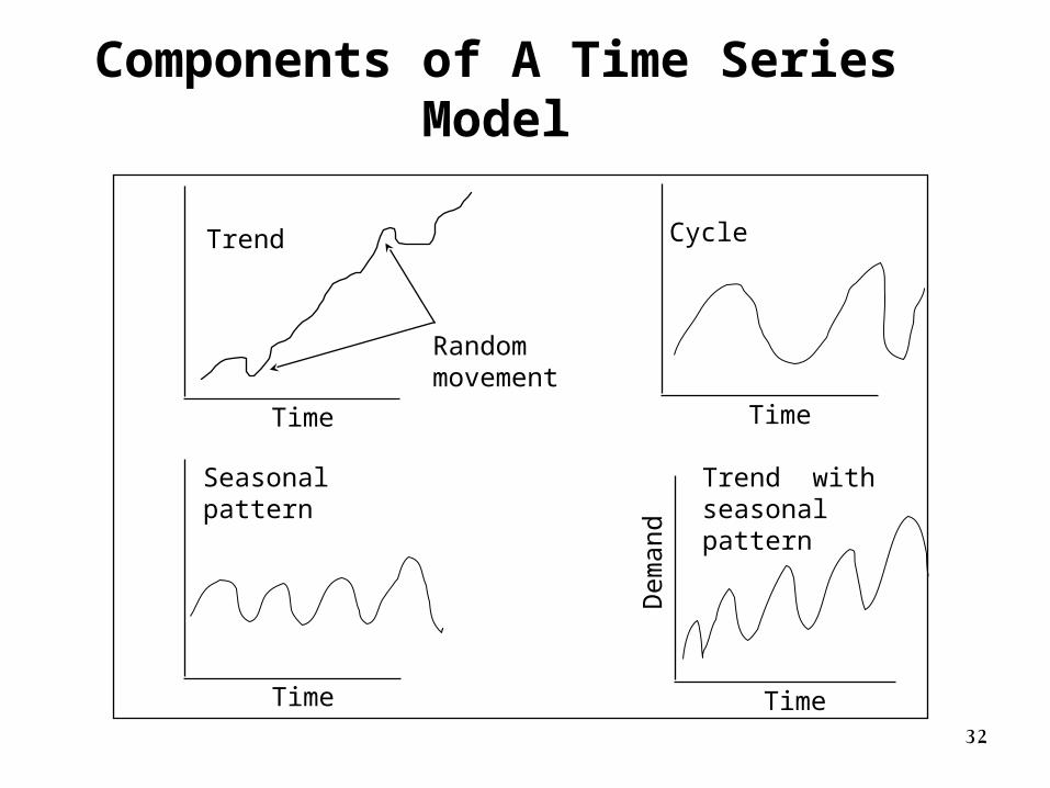
Components of A Time Series Model

Time

Trend

Randommovement

Time

Cycle

Time

Seasonalpattern

Dem

and

Time

Trend with seasonal pattern

33

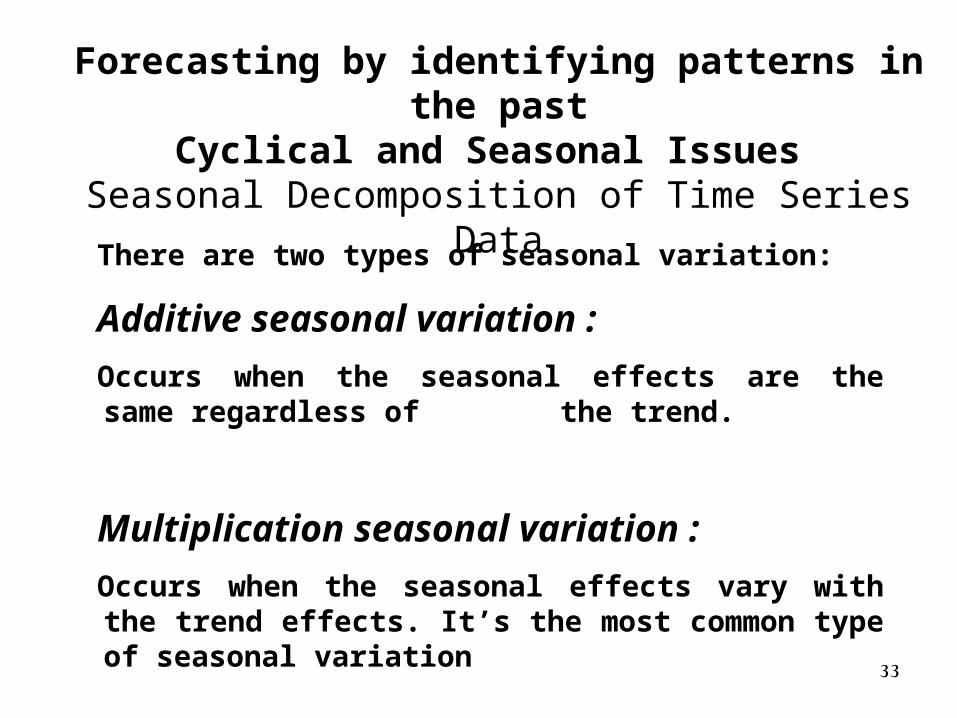
There are two types of seasonal variation:

Additive seasonal variation :

Occurs when the seasonal effects are the same regardless of the trend.

Multiplication seasonal variation :

Occurs when the seasonal effects vary with the trend effects. It’s the most common type of seasonal variation

Forecasting by identifying patterns in the pastCyclical and Seasonal Issues

Seasonal Decomposition of Time Series Data

34

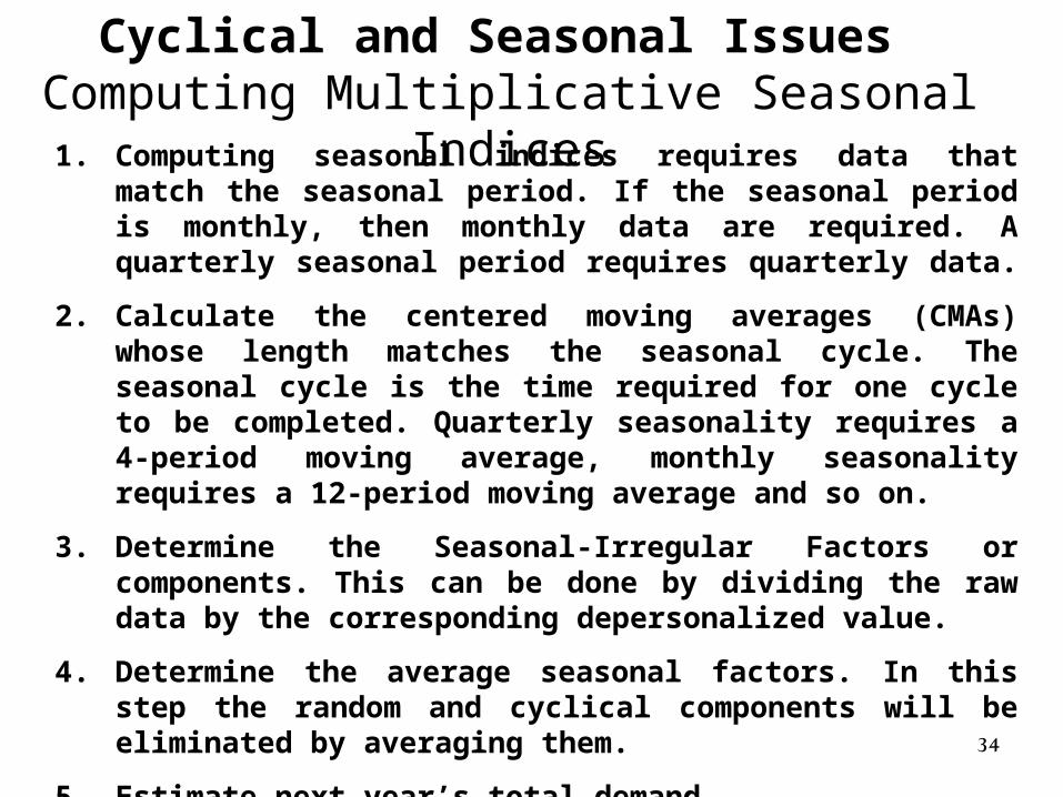
1. Computing seasonal indices requires data that match the seasonal period. If the seasonal period is monthly, then monthly data are required. A quarterly seasonal period requires quarterly data.

2. Calculate the centered moving averages (CMAs) whose length matches the seasonal cycle. The seasonal cycle is the time required for one cycle to be completed. Quarterly seasonality requires a 4-period moving average, monthly seasonality requires a 12-period moving average and so on.

3. Determine the Seasonal-Irregular Factors or components. This can be done by dividing the raw data by the corresponding depersonalized value.

4. Determine the average seasonal factors. In this step the random and cyclical components will be eliminated by averaging them.

5. Estimate next year’s total demand

6. Divide this estimate of total demand by the number of seasons, then multiply it by the seasonal index for that season

Cyclical and Seasonal Issues Computing Multiplicative Seasonal Indices

35

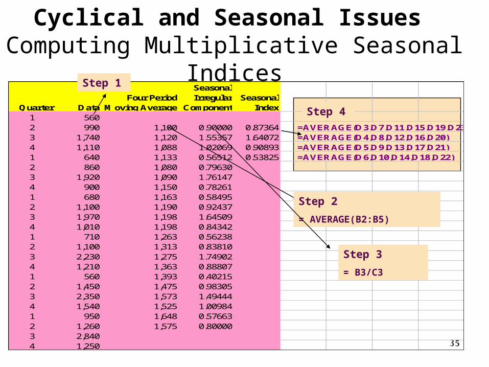
Cyclical and Seasonal Issues Computing Multiplicative Seasonal Indices

Quarter DataFour Period

Moving Average

Seasonal Irregular

ComponentSeasonal

Index1 5602 990 1,100 0.90000 0.873643 1,740 1,120 1.55357 1.640724 1,110 1,088 1.02069 0.908931 640 1,133 0.56512 0.538252 860 1,080 0.796303 1,920 1,090 1.761474 900 1,150 0.782611 680 1,163 0.584952 1,100 1,190 0.924373 1,970 1,198 1.645094 1,010 1,198 0.843421 710 1,263 0.562382 1,100 1,313 0.838103 2,230 1,275 1.749024 1,210 1,363 0.888071 560 1,393 0.402152 1,450 1,475 0.983053 2,350 1,573 1.494444 1,540 1,525 1.009841 950 1,648 0.576632 1,260 1,575 0.800003 2,8404 1,250

=AVERAGE(D3,D7,D11,D15,D19,D23)=AVERAGE(D4,D8,D12,D16,D20)=AVERAGE(D5,D9,D13,D17,D21)=AVERAGE(D6,D10,D14,D18,D22)

Step 2

= AVERAGE(B2:B5)

Step 3

= B3/C3

Step 1

Step 4

36

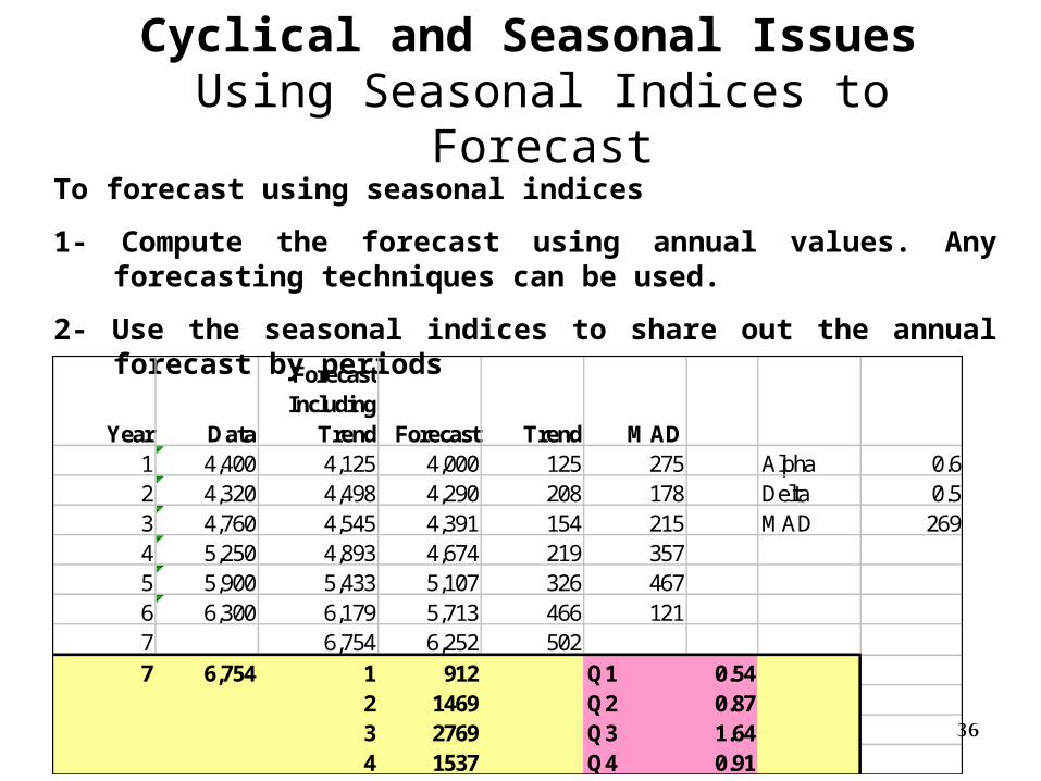
Cyclical and Seasonal Issues Using Seasonal Indices to Forecast

To forecast using seasonal indices

1- Compute the forecast using annual values. Any forecasting techniques can be used.

2- Use the seasonal indices to share out the annual forecast by periods

Year Data

Forecast Including

Trend Forecast Trend MAD1 4,400 4,125 4,000 125 275 Alpha 0.62 4,320 4,498 4,290 208 178 Delta 0.53 4,760 4,545 4,391 154 215 MAD 2694 5,250 4,893 4,674 219 3575 5,900 5,433 5,107 326 4676 6,300 6,179 5,713 466 1217 6,754 6,252 5027 6,754 1 912 Q1 0.54

2 1469 Q2 0.873 2769 Q3 1.644 1537 Q4 0.91

37

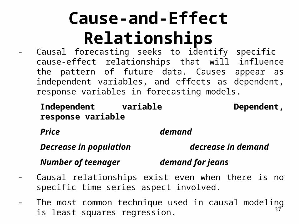
Cause-and-Effect Relationships- Causal forecasting seeks to identify specific cause-effect relationships

that will influence the pattern of future data. Causes appear as independent variables, and effects as dependent, response variables in forecasting models.

Independent variable Dependent, response variable

Price demand

Decrease in population decrease in demand

Number of teenager demand for jeans

- Causal relationships exist even when there is no specific time series aspect involved.

- The most common technique used in causal modeling is least squares regression.

38

Linear Trend analysis

45

55

65

75

85

0 1 2 3 4

D1

D3D2

45

55

65

75

85

0 1 2 3 4

D1D3

D2

P1=80

P2=68

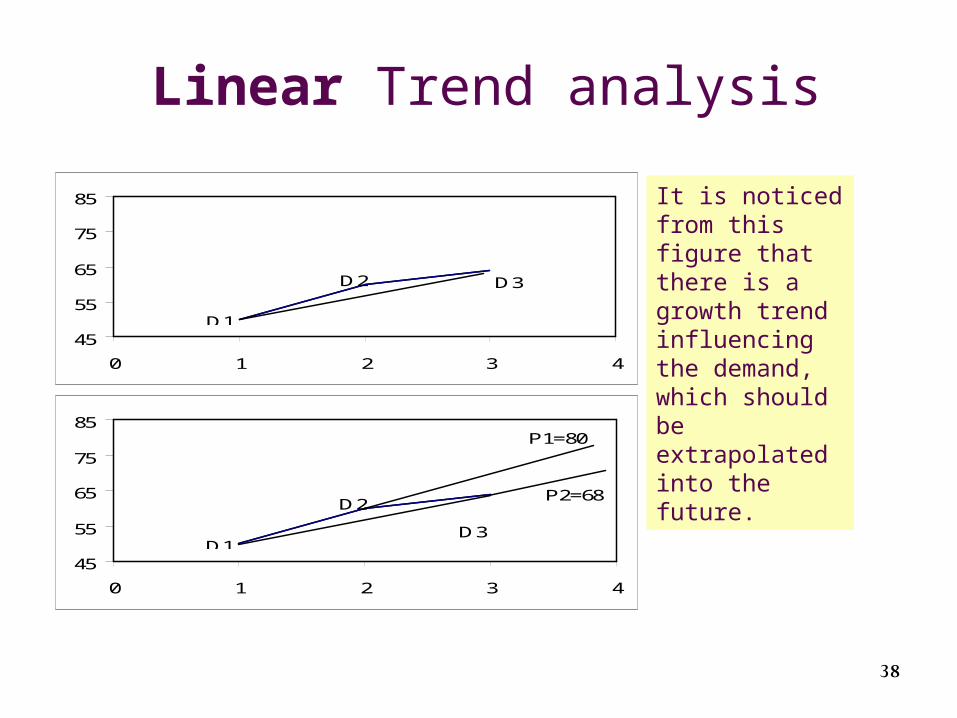
It is noticed from this figure that there is a growth trend influencing the demand, which should be extrapolated into the future.

39

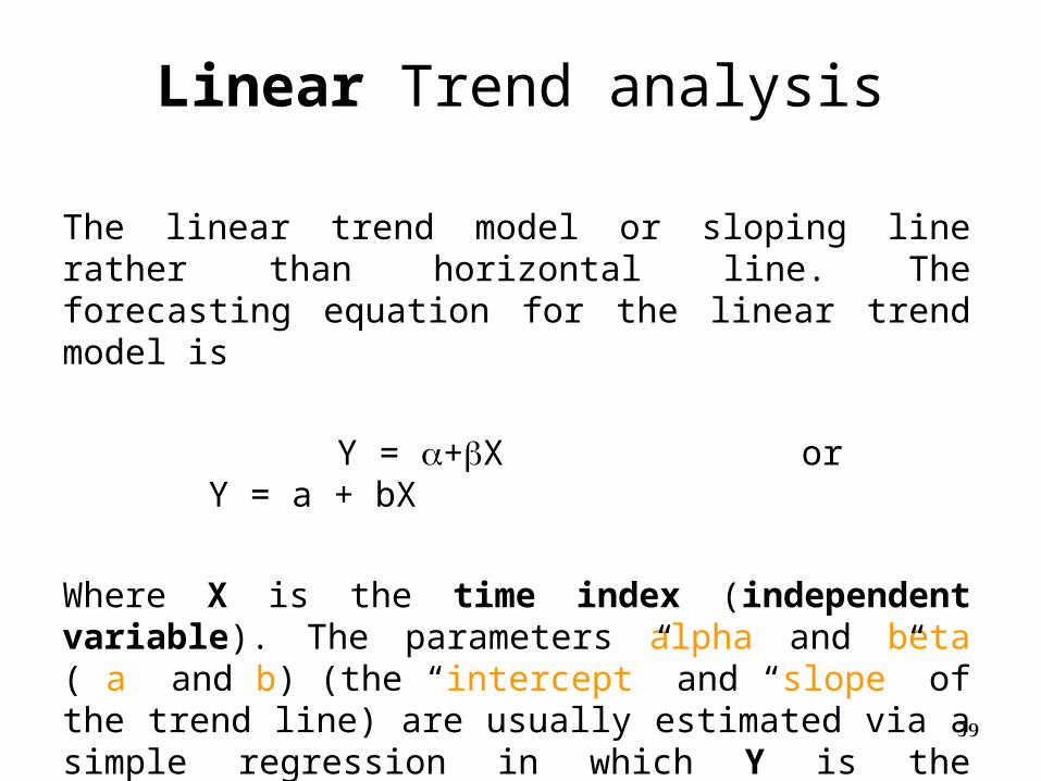
The linear trend model or sloping line rather than horizontal line. The forecasting equation for the linear trend model is

Y = +X or Y = a + bX

Where X is the time index (independent variable). The parameters alpha and beta ( a and b) (the “intercept” and “slope” of the trend line) are usually estimated via a simple regression in which Y is the dependent variable and the time index t is the independent variable.


40

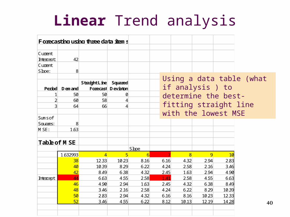
Forecasting using three data items

Current Intercept: 42Current Slope: 8

Period DemandStraight Line

ForecastSquared

Deviaton1 50 50 02 60 58 43 64 66 4

Sums of Squares: 8MSE: 1.63

Table of MSESlope

1.632993 4 5 6 7 8 9 1038 12.33 10.23 8.16 6.16 4.32 2.94 2.8340 10.39 8.29 6.22 4.24 2.58 2.16 3.4642 8.49 6.38 4.32 2.45 1.63 2.94 4.90

Intercept 44 6.63 4.55 2.58 1.41 2.58 4.55 6.6346 4.90 2.94 1.63 2.45 4.32 6.38 8.4948 3.46 2.16 2.58 4.24 6.22 8.29 10.3950 2.83 2.94 4.32 6.16 8.16 10.23 12.3352 3.46 4.55 6.22 8.12 10.13 12.19 14.28


Using a data table (what if analysis ) to determine the best-fitting straight line with the lowest MSE

41

Linear Trend analysis Simple Linear Regression Analysis

Regression analysis is a statistical method of taking one or more variable called independent or predictor variable- and developing a mathematical equation that show how they relate to the value of a single variable- called the dependent variable.

Regression analysis applies least-squares analysis to find the best-fitting line, where best is defined as minimizing the mean square error (MSE) between the historical sample and the calculated forecast.

Regression analysis is one of the tools provided by Excel.

42

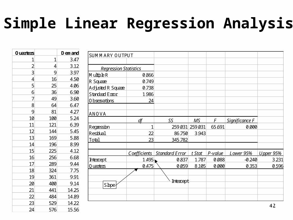
Simple Linear Regression Analysis

Quarters Demand1 1 3.472 4 3.123 9 3.974 16 4.505 25 4.066 36 6.907 49 3.608 64 6.479 81 4.27

10 100 5.2411 121 6.3912 144 5.4513 169 5.8814 196 8.9915 225 4.1216 256 6.6817 289 9.4418 324 7.7519 361 9.9120 400 9.1421 441 14.2522 484 14.8923 529 14.2224 576 15.56

SUMMARY OUTPUT

Regression StatisticsMultiple R 0.866R Square 0.749Adjusted R Square 0.738Standard Error 1.986Observations 24

ANOVAdf SS MS F Significance F

Regression 1 259.031 259.031 65.691 0.000Residual 22 86.750 3.943Total 23 345.782

Coefficients Standard Error t Stat P-value Lower 95% Upper 95%Intercept 1.495 0.837 1.787 0.088 -0.240 3.231Quarters 0.475 0.059 8.105 0.000 0.353 0.596

InterceptSlope

43

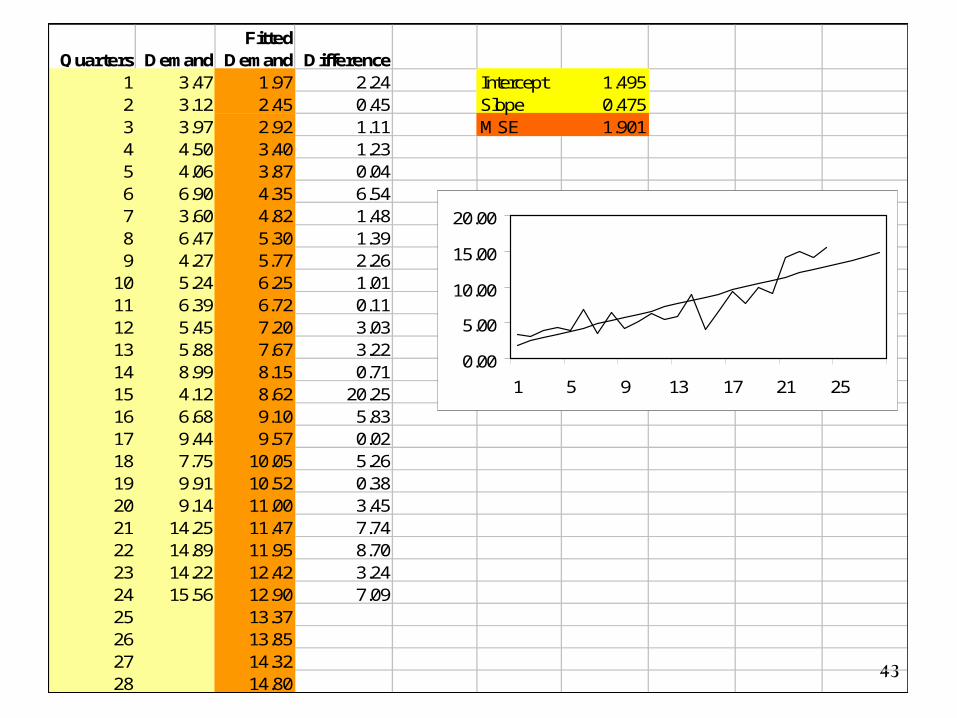
Quarters DemandFitted

Demand Difference1 3.47 1.97 2.24 Intercept 1.4952 3.12 2.45 0.45 Slope 0.4753 3.97 2.92 1.11 MSE 1.9014 4.50 3.40 1.235 4.06 3.87 0.046 6.90 4.35 6.547 3.60 4.82 1.488 6.47 5.30 1.399 4.27 5.77 2.26

10 5.24 6.25 1.0111 6.39 6.72 0.1112 5.45 7.20 3.0313 5.88 7.67 3.2214 8.99 8.15 0.7115 4.12 8.62 20.2516 6.68 9.10 5.8317 9.44 9.57 0.0218 7.75 10.05 5.2619 9.91 10.52 0.3820 9.14 11.00 3.4521 14.25 11.47 7.7422 14.89 11.95 8.7023 14.22 12.42 3.2424 15.56 12.90 7.0925 13.3726 13.8527 14.3228 14.80

0.00

5.00

10.00

15.00

20.00

1 5 9 13 17 21 25

44

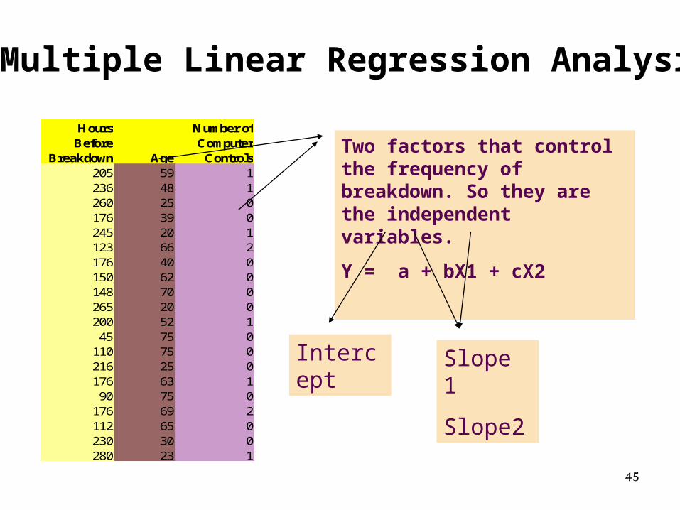
Linear Trend analysis Multiple Linear Regression Analysis

Simple linear regression analysis use one variable (quarter number) as the independent variable in order to predict the future value. In many situations, it is advantageous to use more than one independent variable in a forecast.

45

Hours Before

Breakdown Age

Number of Computer

Controls205 59 1236 48 1260 25 0176 39 0245 20 1123 66 2176 40 0150 62 0148 70 0265 20 0200 52 1

45 75 0110 75 0216 25 0176 63 1

90 75 0176 69 2112 65 0230 30 0280 23 1

Two factors that control the frequency of breakdown. So they are the independent variables.

Y = a + bX1 + cX2

Intercept Slope 1

Slope2

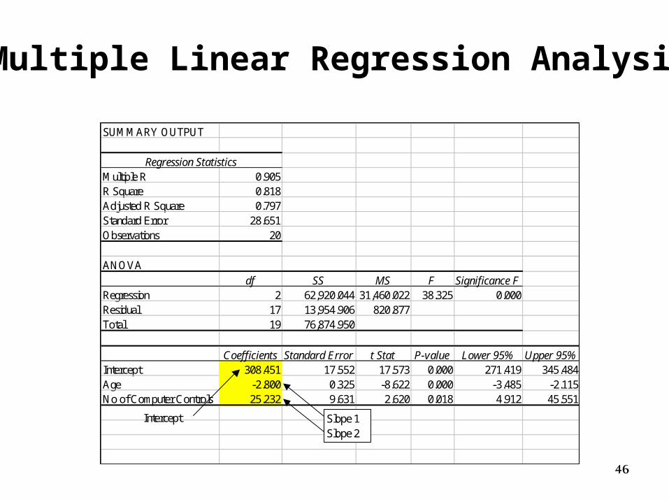
Multiple Linear Regression Analysis

46

SUMMARY OUTPUT



Regression 2 62,920.044 31,460.022 38.325 0.000Residual 17 13,954.906 820.877Total 19 76,874.950

Coefficients Standard Error t Stat P-value Lower 95% Upper 95%Intercept 308.451 17.552 17.573 0.000 271.419 345.484Age -2.800 0.325 -8.622 0.000 -3.485 -2.115No of Computer Controls 25.232 9.631 2.620 0.018 4.912 45.551

Intercept Slope 1Slope 2

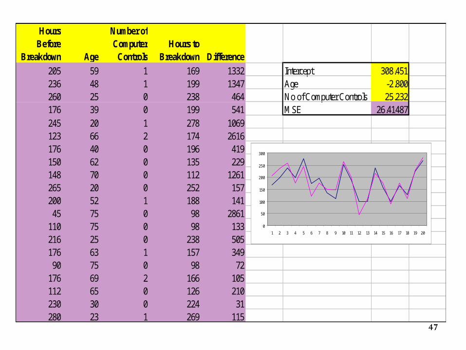
Multiple Linear Regression Analysis

47

Hours Before

Breakdown Age

Number of Computer

ControlsHours to

Breakdown Difference

205 59 1 169 1332 Intercept 308.451236 48 1 199 1347 Age -2.800260 25 0 238 464 No of Computer Controls 25.232176 39 0 199 541 MSE 26.41487245 20 1 278 1069123 66 2 174 2616176 40 0 196 419150 62 0 135 229148 70 0 112 1261265 20 0 252 157200 52 1 188 14145 75 0 98 2861

110 75 0 98 133216 25 0 238 505176 63 1 157 34990 75 0 98 72

176 69 2 166 105112 65 0 126 210230 30 0 224 31280 23 1 269 115

0

50

100

150

200

250

300

1 2 3 4 5 6 7 8 9 10 11 12 13 14 15 16 17 18 19 20

48

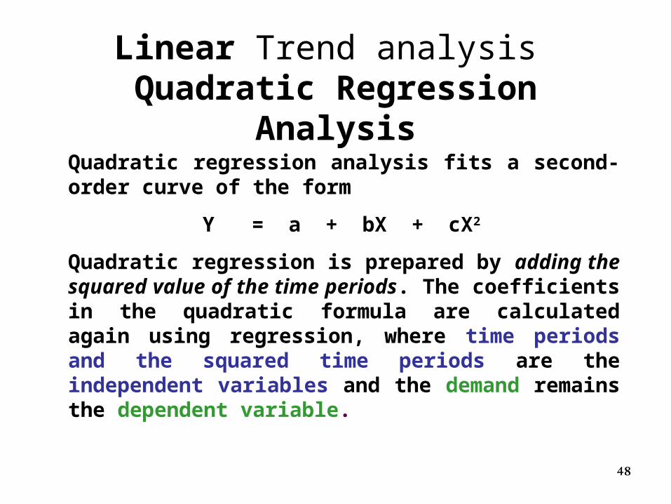
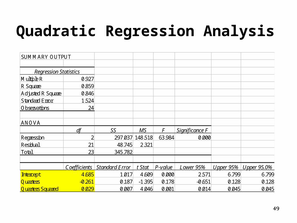
Linear Trend analysis Quadratic Regression Analysis

Quadratic regression analysis fits a second-order curve of the form

Y = a + bX + cX2

Quadratic regression is prepared by adding the squared value of the time periods. The coefficients in the quadratic formula are calculated again using regression, where time periods and the squared time periods are the independent variables and the demand remains the dependent variable.

49

SUMMARY OUTPUT



Regression 2 297.037 148.518 63.984 0.000Residual 21 48.745 2.321Total 23 345.782

Coefficients Standard Error t Stat P-value Lower 95% Upper 95% Upper 95.0%Intercept 4.685 1.017 4.609 0.000 2.571 6.799 6.799Quarters -0.261 0.187 -1.395 0.178 -0.651 0.128 0.128Quarters Squared 0.029 0.007 4.046 0.001 0.014 0.045 0.045

Quadratic Regression Analysis

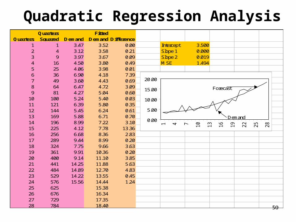
50

Quadratic Regression AnalysisQuarters

Quarters Squared Demand

Fitted Demand Difference

1 1 3.47 3.52 0.00 Intercept 3.5002 4 3.12 3.58 0.21 Slope 1 0.0003 9 3.97 3.67 0.09 Slope 2 0.0194 16 4.50 3.80 0.49 MSE 1.4945 25 4.06 3.98 0.016 36 6.90 4.18 7.397 49 3.60 4.43 0.698 64 6.47 4.72 3.099 81 4.27 5.04 0.60

10 100 5.24 5.40 0.0311 121 6.39 5.80 0.3512 144 5.45 6.24 0.6113 169 5.88 6.71 0.7014 196 8.99 7.22 3.1015 225 4.12 7.78 13.3616 256 6.68 8.36 2.8317 289 9.44 8.99 0.2018 324 7.75 9.66 3.6319 361 9.91 10.36 0.2020 400 9.14 11.10 3.8521 441 14.25 11.88 5.6322 484 14.89 12.70 4.8323 529 14.22 13.55 0.4524 576 15.56 14.44 1.2425 625 15.3826 676 16.3427 729 17.3528 784 18.40

0.00

5.00

10.00

15.00

20.00

1 4 7 10

13

16

19

22

25

28

Demand

Forecast

1 Chapter 2 and 3 Forecasting Advanced Forecasting Operations Analysis Using MS Excel.

Documents

Transcript of 1 Chapter 2 and 3 Forecasting Advanced Forecasting Operations Analysis Using MS Excel.