1 CE 530 Molecular Simulation Lecture 10 Simple Biasing Methods David A. Kofke Department of...
39
1 CE 530 Molecular Simulation Lecture 10 Simple Biasing Methods David A. Kofke Department of Chemical Engineering SUNY Buffalo [email protected]ffalo.edu
-
Upload
marjory-haynes -
Category
Documents
-
view
217 -
download
4
Transcript of 1 CE 530 Molecular Simulation Lecture 10 Simple Biasing Methods David A. Kofke Department of...
1
CE 530 Molecular Simulation
Lecture 10
Simple Biasing Methods
David A. Kofke
Department of Chemical Engineering
SUNY Buffalo

2
ReviewMonte Carlo simulation
• Markov chain to generate elements of ensemble with proper distribution
Metropolis algorithm• relies on microscopic reversibility
• two parts to a Markov step generate trial move (underlying transition probability matrix) decide to accept move or keep original state
Determination of acceptance probabilities• detailed analysis of forward and reverse moves
• we examined molecule displacement and volume-change trials
i ij j ji
3
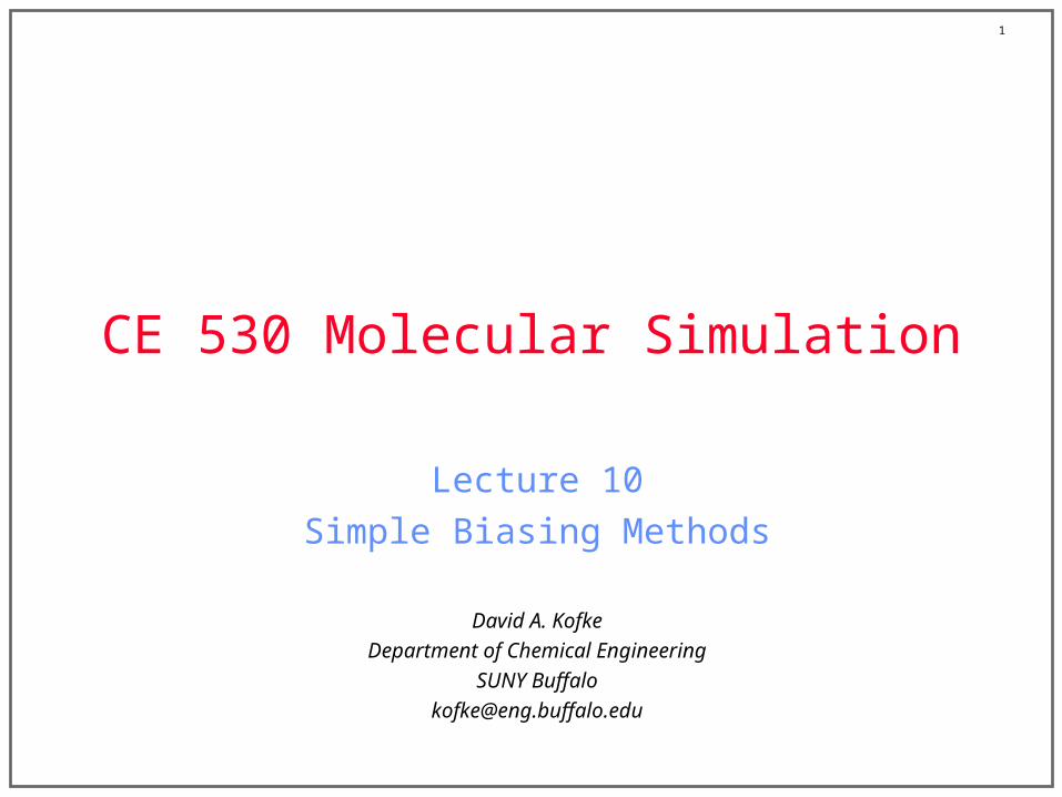
Performance Measures
How do we improve the performance of a MC simulation?• characterization of performance
• means to improve performance
Return to our consideration of a general Markov process• fixed number of well defined states
• fully specified transition-probability matrix
• use our three-state prototype
Performance measures• rate of convergence
• variance in occupancies
11 12 13
21 22 23
31 32 33

4
Rate of Convergence 1.
What is the likely distribution of states after a run of finite length?• Is it close to the limiting distribution?
• We can apply similarity transforms to understand behavior of eigenvector equation
( ) ( ) ( )11 12 13
( ) (0) ( ) ( ) ( ) ( ) ( ) ( )1 1 21 22 23 11 12 13
( ) ( ) ( )31 32 33
1 0 0
n n n
n n n n n n nn
n n n
n
Probability of being in state 3 after n moves, beginning in state 1
1
2
3
0 0
eigenvalue matrix: 0 0
0 0
1 2 3eigenvector matrix
1

5
Rate of Convergence 1.
What is the likely distribution of states after a run of finite length?• Is it close to the limiting distribution?
• We can apply similarity transforms to understand behavior of eigenvector equation
( ) ( ) ( )11 12 13
( ) (0) ( ) ( ) ( ) ( ) ( ) ( )1 1 21 22 23 11 12 13
( ) ( ) ( )31 32 33
1 0 0
n n n
n n n n n n nn
n n n
n
Probability of being in state 3 after n moves, beginning in state 1
1 1 1
1 1
1
... ..(n times) .
...
n
n
1
2
3
0 0
0 0
0 0
n
n n
n
1
6
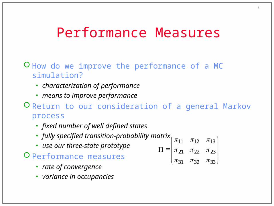
Rate of Convergence 2.
Likely distribution after finite run
Convergence rate determined by magnitude of other eigenvalues• very close to unity indicates slow convergence
1
2 2
3 3
0 0 1 0 0 1 0 0
0 0 0 0 0 0 0
0 0 00 0 0 0
n
n n n
nn n
( ) (0) (0) 1n n ni i i

7
Occupancy Variance 1.
Imagine repeating Markov sequence many times (L), each time taking a fixed number of steps, M• tabulate histogram for each sequence;
• examine variances in occupancy fraction
• through propagation of error, the occupancy (co)variances sum to give the variances in the ensemble averages; e.g. (for a 2-state system)
• we would like these to be small
( )( )
kimk
i Mp
2( )2
1
Lk
i iik
p
1 2
3 4
... L
2 2 2 2 21 1 2 2 1 2 1 22U U U U U
( ) ( )
1
Lk k
i j i ji jk
p p

8
Occupancy Variance 2.
A formula for the occupancy (co)variance is known
• right-hand sides independent of M
• standard deviation decreases as
2 2 2 1 variance
covariance
i i i ii
i j i j i ij j ji
M s
M s s
1/ M
1( )S I

9
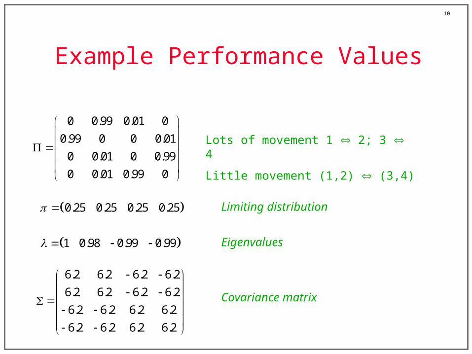
Example Performance Values
0.0 0.5 0.5
0.25 0.5 0.25
0.5 0.5 0.0
0.42 0.33 0.25
0.17 0.66 0.17
0.25 0.33 0.42
0.97 0.02 0.01
0.01 0.98 0.01
0.01 0.02 0.97
0 1 0
0.5 0 0.5
0 1 0
Metropolis
Barker
Inefficient
Most efficient
0.25 0.5 0.25 Limiting distribution
1 0.96 0.96 9.2 6.1 3.1
6.1 12.2 6.1
3.1 6.1 9.2
1 0.33 0.17 0.30 0.25 0.05
0.25 0.50 0.25
0.05 0.25 0.30
1 0 1 0.125 0 0.125
0 0 0
0.125 0 0.125
1 0 0.5 0.10 0.125 0.02
0.125 0.25 0.125
0.02 0.125 0.10
10
Example Performance Values
0 0.99 0.01 0
0.99 0 0 0.01
0 0.01 0 0.99
0 0.01 0.99 0
0.25 0.25 0.25 0.25
1 0.98 0.99 0.99
6.2 6.2 6.2 6.2
6.2 6.2 6.2 6.2
6.2 6.2 6.2 6.2
6.2 6.2 6.2 6.2
Lots of movement 1 2; 3 4
Little movement (1,2) (3,4)
Limiting distribution
Eigenvalues
Covariance matrix

11
Heuristics to Improve Performance
Keep the system moving• minimize diagonal elements of probability matrix
• avoid repeated transitions among a few states
Typical physical situations where convergence is poor• large number of equivalent states with poor transitions between
regions of them entangled polymers
• large number of low-probability states and a few high-probability states low-density associating systems
Low, nonzero probability region
High probability region
Bottleneck
Phase space
12
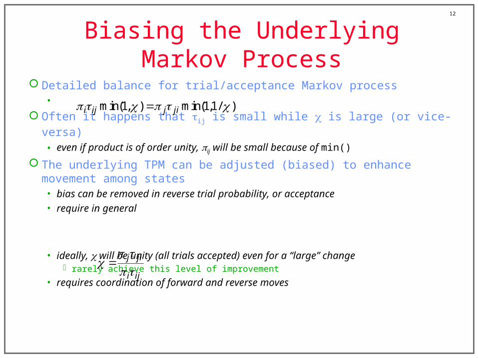
Biasing the Underlying Markov Process
Detailed balance for trial/acceptance Markov process•
Often it happens that ij is small while is large (or vice-versa)
• even if product is of order unity, ij will be small because of min()
The underlying TPM can be adjusted (biased) to enhance movement among states• bias can be removed in reverse trial probability, or acceptance
• require in general
• ideally, will be unity (all trials accepted) even for a “large” change rarely achieve this level of improvement
• requires coordination of forward and reverse moves
min(1, ) min(1,1/ )i ij j ji
j ji
i ij

13
Example: Biased Insertion in GCMC
Grand-canonical Monte Carlo (VT)• fluctuations in N require insertion/deletion trials
• at high density, insertions may be rarely accepted ij is small for j a state with additional, non-overlapping molecule
• at high chemical potential, limiting distribution strongly favors additional molecules is large for (N+1) state with no overlap
• apply biasing to improve acceptance
• first look at unbiased algorithm
Ne
14
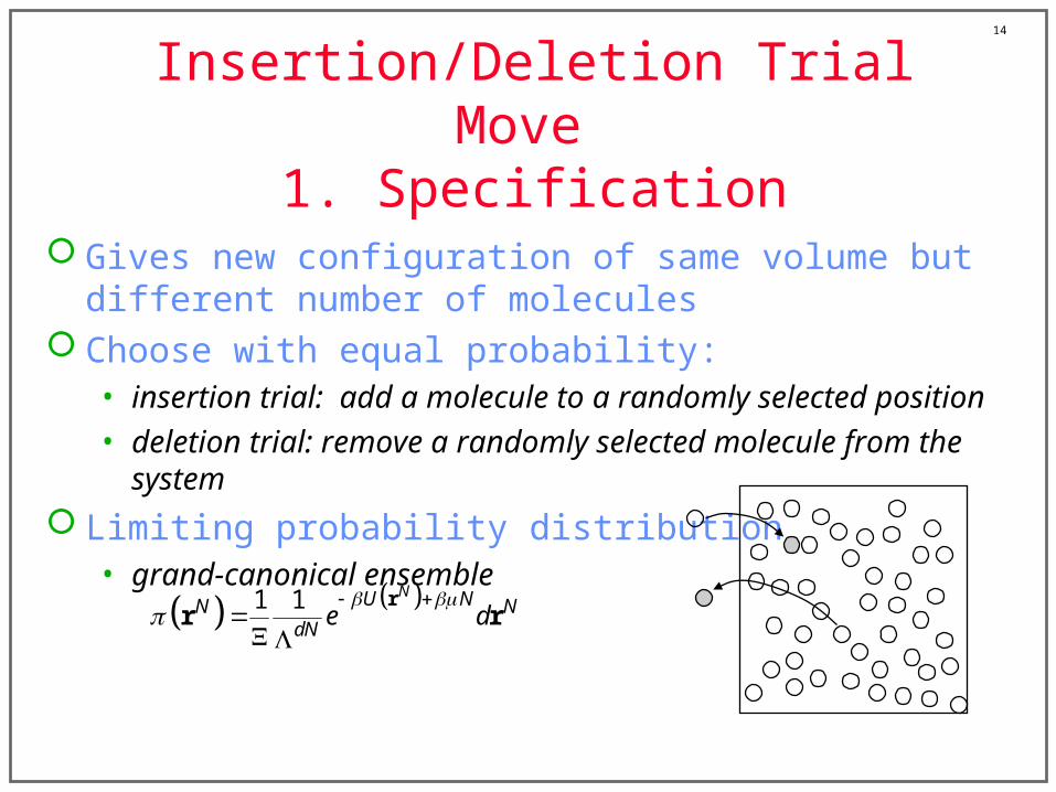
Insertion/Deletion Trial Move 1. Specification
Gives new configuration of same volume but different number of molecules
Choose with equal probability:• insertion trial: add a molecule to a randomly selected position
• deletion trial: remove a randomly selected molecule from the system
Limiting probability distribution• grand-canonical ensemble
1 1 NU NN NdN
e d
rr r

15
Insertion/Deletion Trial Move 2. Analysis of Trial Probabilities
Detailed specification of trial moves and and probabilities
Event[reverse event]
Probability[reverse probability]
Select insertion trial[select deletion trial]
½[½ ]
Place molecule at rN+1
[delete molecule N+1]dr/V
[1/(N+1)]
Accept move[accept move]
min(1,)[min(1,1/)]
Forward-step trial probability
1min(1, )
2
d
V
r
Reverse-step trial probability
11 1min(1, )
2 1N
is formulated to satisfy detailed balance

16
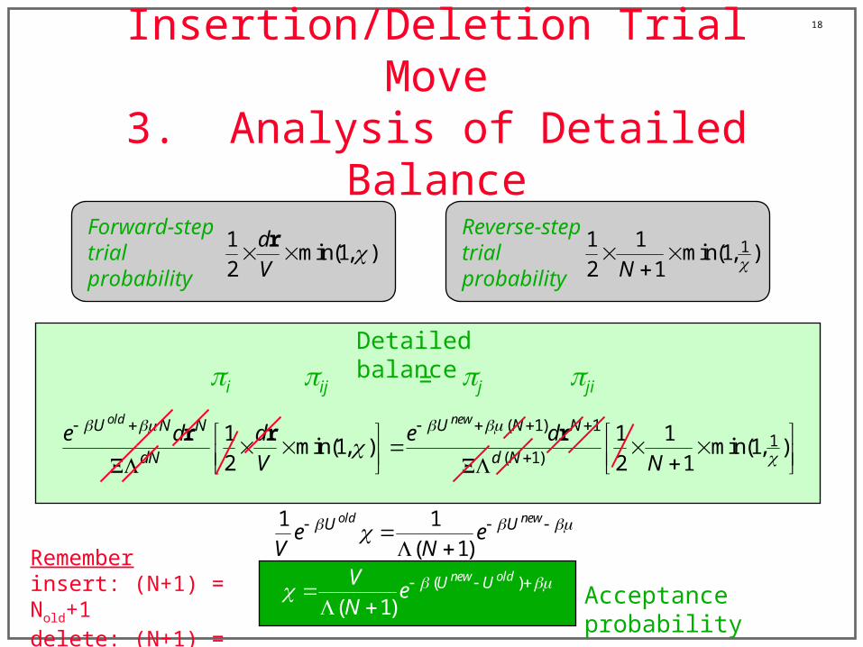
Insertion/Deletion Trial Move3. Analysis of Detailed Balance
Detailed balance
i ij j ji=
Limiting distribution 1 1 NU NN N
dNe d
rr r
Forward-step trial probability
1min(1, )
2
d
V
rReverse-step trial probability
11 1min(1, )
2 1N
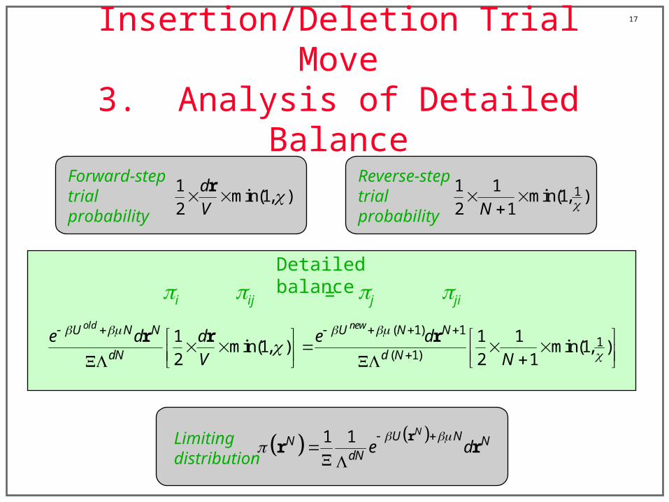
17
Insertion/Deletion Trial Move3. Analysis of Detailed Balance
Detailed balance
( 1) 11
( 1)
1 1 1min(1, ) min(1, )
2 2 1
old newU N N U N N
dN d N
e d d e d
V N
r r r
i ij j ji=
Forward-step trial probability
1min(1, )
2
d
V
rReverse-step trial probability
11 1min(1, )
2 1N
Limiting distribution 1 1 NU NN N
dNe d
rr r
18
Insertion/Deletion Trial Move3. Analysis of Detailed Balance
Detailed balance
( 1) 11
( 1)
1 1 1min(1, ) min(1, )
2 2 1
old newU N N U N N
dN d N
e d d e d
V N
r r r
i ij j ji=
Forward-step trial probability
1min(1, )
2
d
V
rReverse-step trial probability
11 1min(1, )
2 1N
1 1
( 1)
old newU Ue eV N
( )
( 1)
new oldU UVe
N
Acceptance probability
Rememberinsert: (N+1) = Nold+1delete: (N+1) = Nold
19
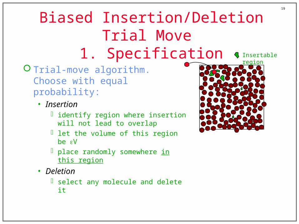
Biased Insertion/Deletion Trial Move 1. Specification
Trial-move algorithm. Choose with equal probability:• Insertion
identify region where insertion will not lead to overlap
let the volume of this region be V place randomly somewhere in this region
• Deletion select any molecule and delete it
Insertable region
20
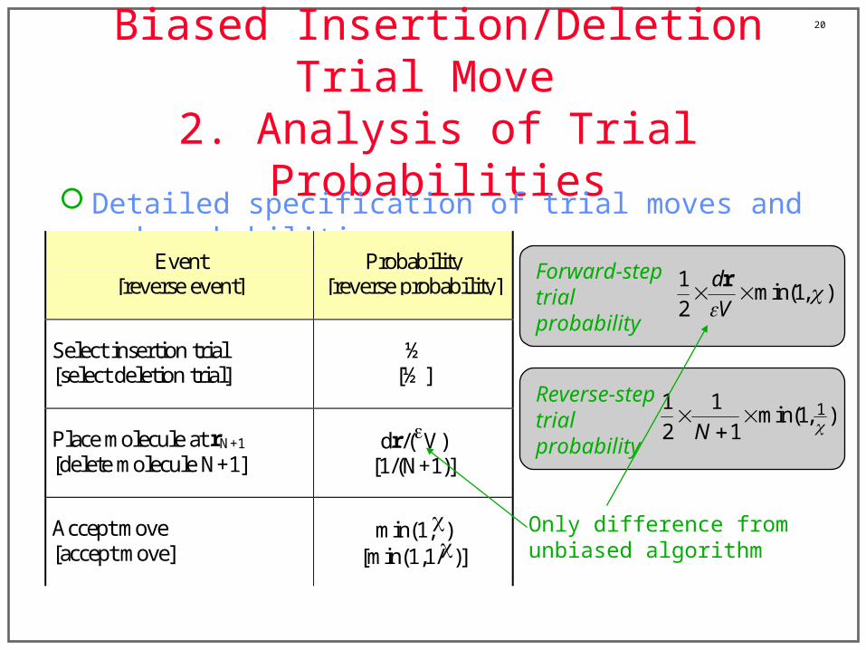
Biased Insertion/Deletion Trial Move 2. Analysis of Trial Probabilities
Detailed specification of trial moves and and probabilities
Event[reverse event]
Probability[reverse probability]
Select insertion trial[select deletion trial]
½[½ ]
Place molecule at rN+1
[delete molecule N+1]dr/(V)
[1/(N+1)]
Accept move[accept move]
min(1,)[min(1,1/)]
Forward-step trial probability
1min(1, )
2
d
V
r
Reverse-step trial probability
11 1min(1, )
2 1N
Only difference from unbiased algorithm

21
Biased Insertion/Deletion Trial Move3. Analysis of Detailed Balance
Detailed balance
( 1) 11
( 1)
1 1 1min(1, ) min(1, )
2 2 1
old newU N N U N N
dN d N
e d d e d
V N
r r r
i ij j ji=
( )
( 1)
new oldU UVe
N
Acceptance probability
Rememberinsert: (N+1) = Nold+1delete: (N+1) = Nold
• must be computed even when doing a deletion, since depends upon it for deletion, is computed for configuration after molecule is removed for insertion is computed for configuration before molecule is inserted
22
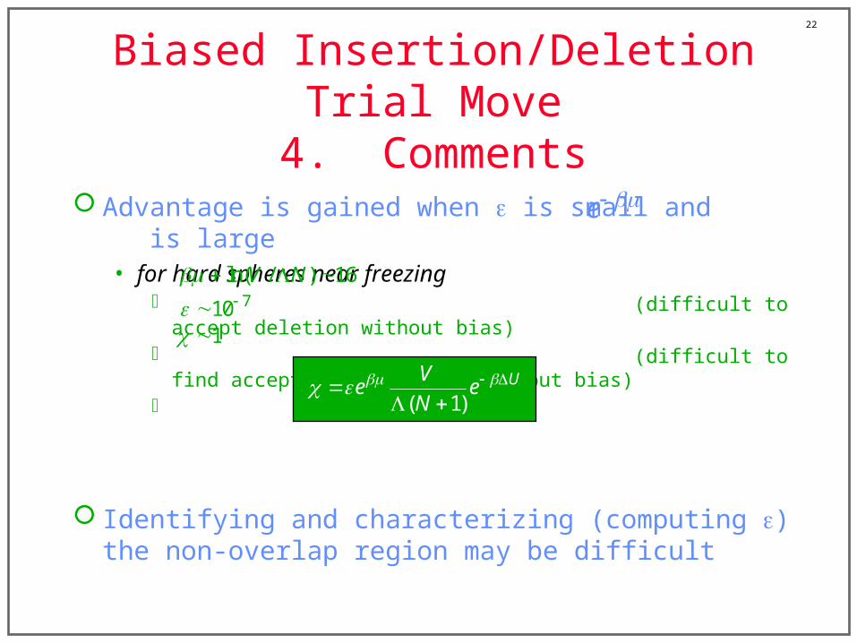
Advantage is gained when is small and is large• for hard spheres near freezing
(difficult to accept deletion without bias) (difficult to find acceptable insertion without bias)
Identifying and characterizing (computing ) the non-overlap region may be difficult
Biased Insertion/Deletion Trial Move4. Comments
( 1)UV
e eN
e
ln( / ) 16V N 710
1
23
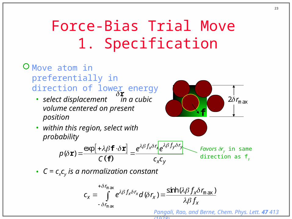
Force-Bias Trial Move 1. Specification
Move atom in preferentially in direction of lower energy• select displacement in a
cubic volume centered on present position
• within this region, select with probability
• C = cxcy is a normalization constant
exp( )
y yx x f rf r
x y
e ep
C c c
f rr
f
f
r
Favors ry in same direction as fy
max
max
maxsinh( )( )x x
rf r x
x xxr
f rc e d r
f
max2 r
Pangali, Rao, and Berne, Chem. Phys. Lett. 47 413 (1978)

24
An Aside: Sampling from a Distribution Rejection method for sampling from a complex distribution p(x)
• write p(x) = Ca(x)b(x) a(x) is a simpler distribution b(x) lies between zero and unity
• recipe generate a uniform random variate U on (0,1) generate a variate X on the distribution a(x) if U b(X) then keep X if not, try again with a new U and X
We wish to sample from p(x) = eqx for x = (-d,d)• we know how to sample on eq(x-x0) for x = (x0,)
• use rejection method with a(x) = eq(x-d)
b(x) = 0 for x < -d or x > +d; 1 otherwise– i.e., sample on a(x) and reject values outside desired range
0 ln[ (0,1)]x x q U
25
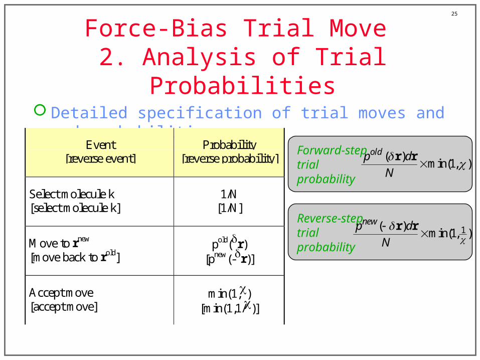
Force-Bias Trial Move 2. Analysis of Trial Probabilities
Detailed specification of trial moves and and probabilities
Event[reverse event]
Probability[reverse probability]
Select molecule k[select molecule k]
1/N[1/N]
Move to rnew
[move back to rold]pold(r)
[pnew(-r)]
Accept move[accept move]
min(1,)[min(1,1/)]
Forward-step trial probability
( )min(1, )
oldp d
N
r r
Reverse-step trial probability
1( )min(1, )
newp d
N r r
26
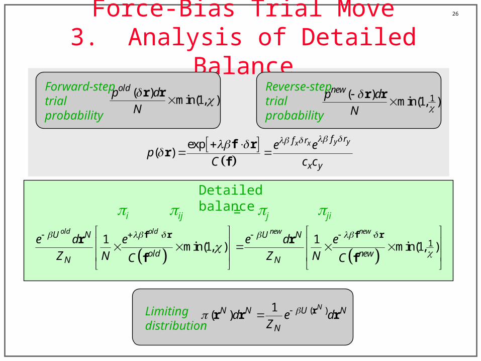
Force-Bias Trial Move3. Analysis of Detailed Balance
Detailed balance
11 1
min(1, ) min(1, )
old old new newU N U N
old newN N
e d e e d e
Z N Z NC C
f r f rr r
f f
i ij j ji=
Limiting distribution
( )1( )
NN N U N
Nd e d
Z rr r r
Forward-step trial probability
( )min(1, )
oldp d
N
r r Reverse-step trial probability
1( )min(1, )
newp d
N r r
exp( )
y yx x f rf r
x y
e ep
C c c
f rr
f
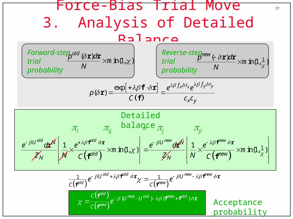
27
Force-Bias Trial Move3. Analysis of Detailed Balance
1 1
old old new new
old newU U
C Ce e f r f r
f f
( ) ( )old
new old new old
new
C U U
Ce
f f f r
fAcceptance probability
Detailed balance
11 1
min(1, ) min(1, )
old old new newU N U N
old newN N
e d e e d e
Z N Z NC C
f r f rr r
f f
i ij j ji=
Forward-step trial probability
( )min(1, )
oldp d
N
r r Reverse-step trial probability
1( )min(1, )
newp d
N r r
exp( )
y yx x f rf r
x y
e ep
C c c
f rr
f

28
Necessary to compute force both before and after move
From definition of force•
• = 1/2 makes argument of exponent nearly zero
• = 0 reduces to unbiased case
Force-bias makes Monte Carlo more like molecular dynamics• example of hybrid MC/MD method
Improvement in convergence by factor or 2-3 observed• worth the effort?
Force-Bias Trial Move4. Comments
( ) ( )old
new old new old
new
C U U
Ce
f f f r
f
12
( )new old new oldU U f f r
U f

29
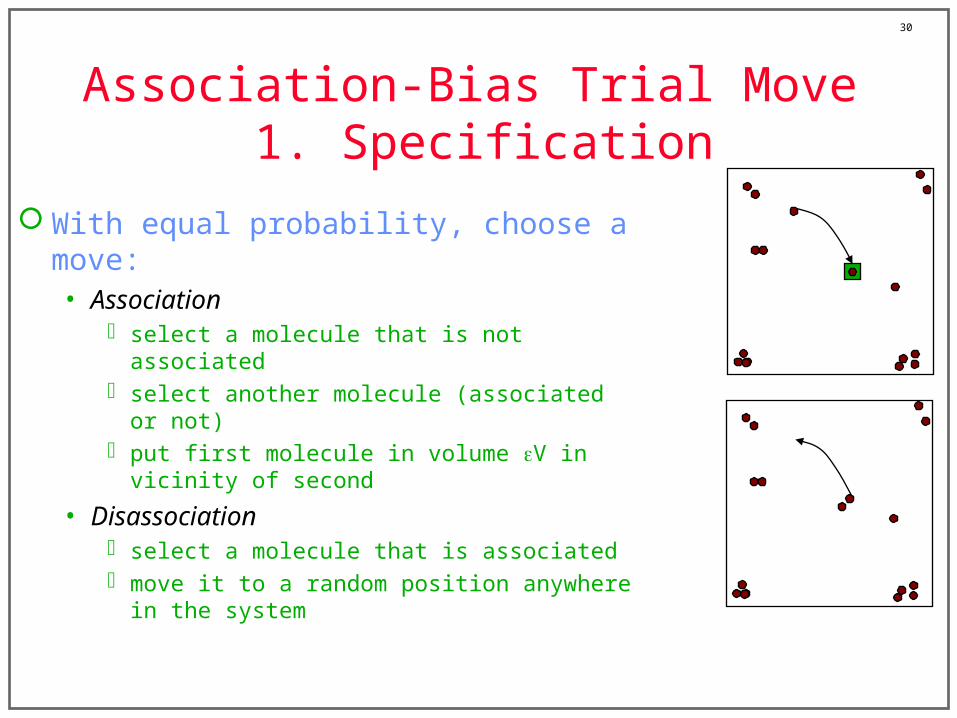
Association-Bias Trial Move 1. Specification
Low-density, strongly attracting molecules• when together, form strong associations that take
long to break
• when apart, are slow to find each other to form associations
• performance of simulation is a problem
Perform moves that put one molecule preferentially in vicinity of another• suffer overlaps, maybe 50% of time
• compare to problem of finding associate only 1 time in (say) 1000
Must also preferentially attempt reverse move
Attempt placement in this region, of volume V
30
Association-Bias Trial Move 1. Specification
With equal probability, choose a move:• Association
select a molecule that is not associated select another molecule (associated or not) put first molecule in volume V in vicinity of
second
• Disassociation select a molecule that is associatedmove it to a random position anywhere in the
system

31
Association-Bias Trial Move 2. Analysis of Trial Probabilities
Detailed specification of trial moves and and probabilities
Event[reverse event]
Probability[reverse probability]
Select molecule k[select molecule k]
1/Nun
[1/Nassoc]
Move to rnew
[move back to rold]1/{(Nassoc+1)V} (*)
[1/V]
Accept move[accept move]
min(1,)[min(1,1/)]
Forward-step trial probability
1min(1, )
( 1)u aN N V
Reverse-step trial probability
11min(1, )
aN V
(*) incorrect
32
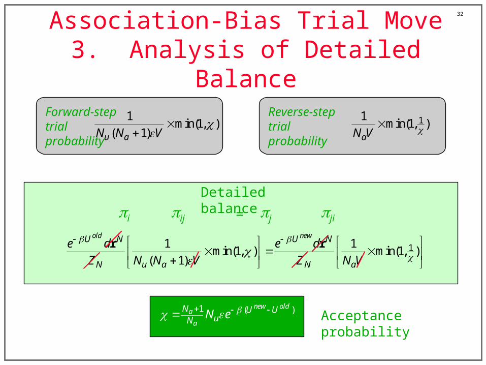
Association-Bias Trial Move3. Analysis of Detailed Balance
1 ( )new olda
a
N U UuN
N e Acceptance probability
Detailed balance
11 1min(1, ) min(1, )
( 1)
old newU N U N
N u a N a
e d e d
Z N N V Z N V
r r
i ij j ji=
Forward-step trial probability
Reverse-step trial probability
11min(1, )
aN V 1
min(1, )( 1)u aN N V

33
This is incorrect!
Need to account for full probability of positioning in rnew
• must look in local environment of trial position to see if it lies also in the neighborhood of other atoms add a 1/V for each atom
Algorithm requires to identify or keep track of number of associated/unassociated molecules
Association-Bias Trial Move4. Comments
1 ( )new olda
a
N U UuN
N e
This region has extra probability of being selected (in vicinity of two molecules)
34
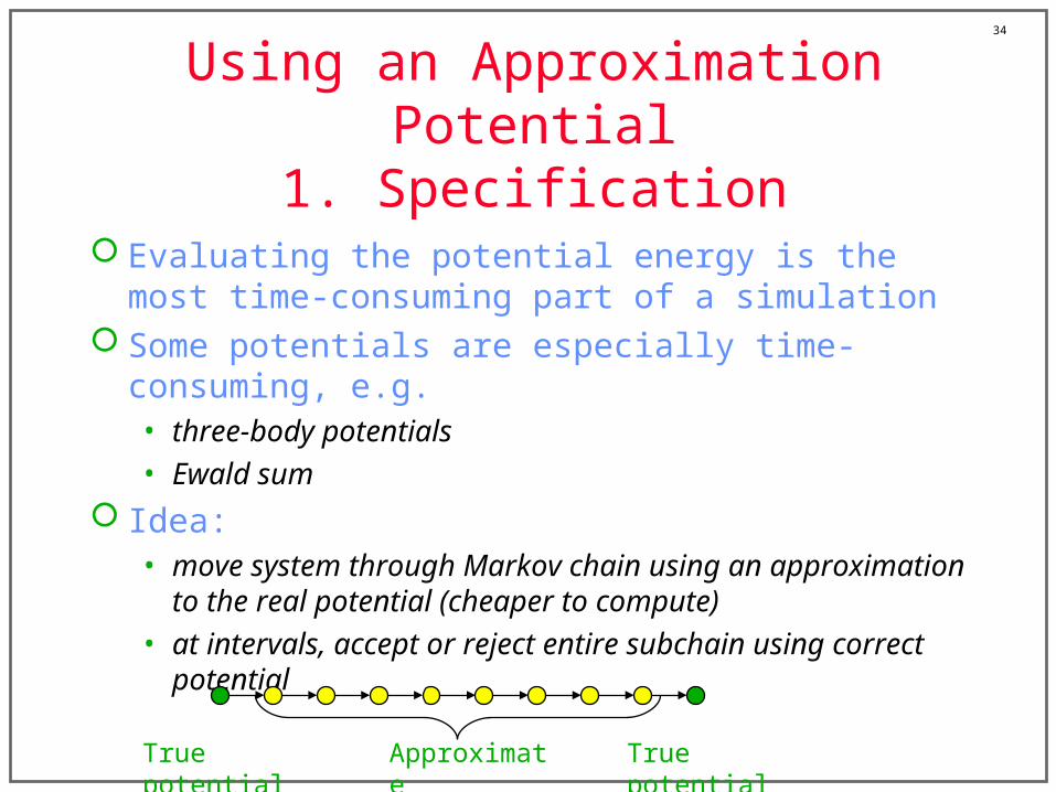
Using an Approximation Potential1. Specification
Evaluating the potential energy is the most time-consuming part of a simulation
Some potentials are especially time-consuming, e.g.• three-body potentials
• Ewald sum
Idea: • move system through Markov chain using an approximation to
the real potential (cheaper to compute)
• at intervals, accept or reject entire subchain using correct potential
True potential Approximate True potential

35
Approximation Potential 2. Analysis of Trial Probabilities
What are ij and ji?
Given that each elementary Markov step obeys detailed balance for the approximate potential… • …one can show that the “super-step” i j also obeys detailed
balance (for the approximate potential)
•
• very hard to analyze without this resultwould have to consider all paths from i to j to get transition probability
1 2 3 n
State i State j
( ) ( )n na ai jij ji

36
Approximation Potential3. Analysis of Detailed Balance
Formulate acceptance criterion to satisfy detailed balance for the real potential
1 2 3 n
State i State j
( ) ( )n na ai jij ji
( ) ( )min(1, ) min(1,1/ )n ni jij ji Approximate-potential
detailed balance
( ( )) min(1, ) min(1,1/ )aj n
jiai
ni j ji
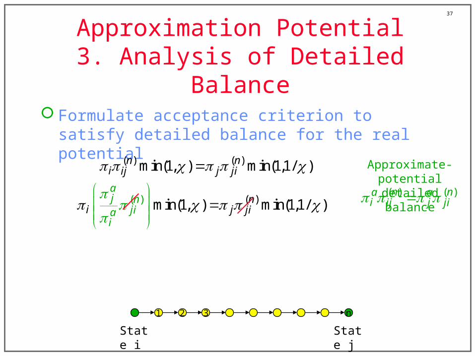
37
Approximation Potential3. Analysis of Detailed Balance
Formulate acceptance criterion to satisfy detailed balance for the real potential
1 2 3 n
State i State j
( ) ( )n na ai jij ji
( ) ( )min(1, ) min(1,1/ )n ni jij ji Approximate-potential
detailed balance
( ( )) min(1, ) min(1,1/ )aj n
jiai
ni j ji
38
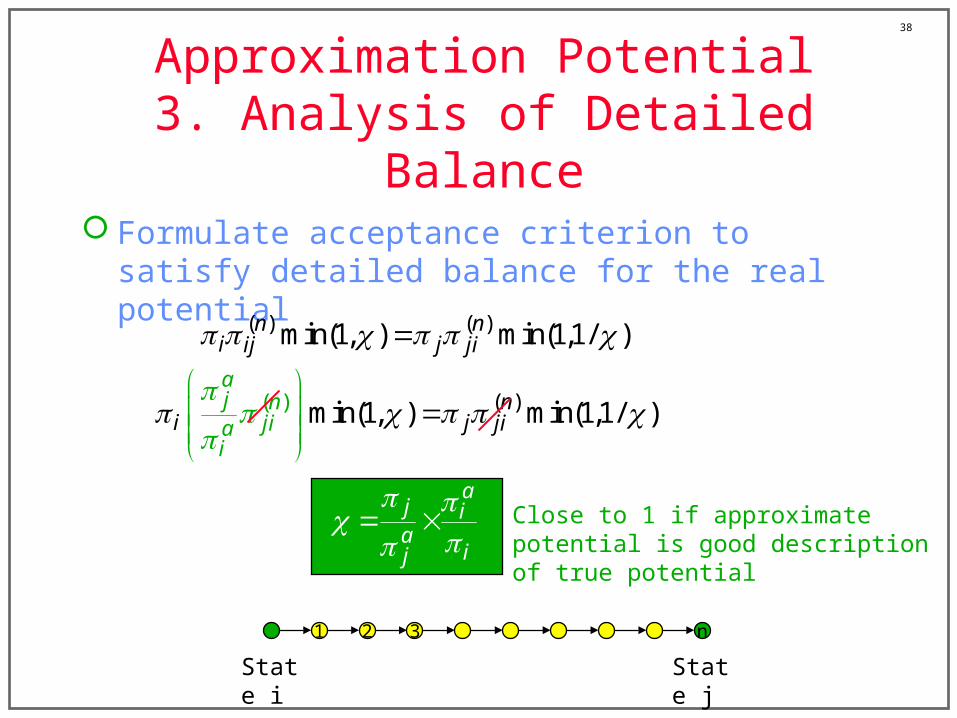
Approximation Potential3. Analysis of Detailed Balance
Formulate acceptance criterion to satisfy detailed balance for the real potential
1 2 3 n
State i State j
( ) ( )min(1, ) min(1,1/ )n ni jij ji
Close to 1 if approximate potential is good description of true potential
( ( )) min(1, ) min(1,1/ )aj n
jiai
ni j ji
aj ia
ij
39
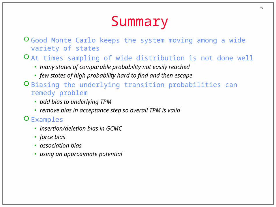
Summary Good Monte Carlo keeps the system moving among a wide variety of states At times sampling of wide distribution is not done well
• many states of comparable probability not easily reached
• few states of high probability hard to find and then escape
Biasing the underlying transition probabilities can remedy problem• add bias to underlying TPM
• remove bias in acceptance step so overall TPM is valid
Examples• insertion/deletion bias in GCMC
• force bias
• association bias
• using an approximate potential