1

Calibrating Distributed Camera Networks

Using Belief PropagationDhanya Devarajan and Richard J. Radke∗.

Department of Electrical, Computer, and Systems Engineering

Rensselaer Polytechnic Institute, Troy, NY 12180

devard@rpi.edu,rjradke@ecse.rpi.edu

Abstract

We discuss how to obtain the accurate and globally consistent self-calibration of a distributed camera

network, in which camera nodes with no centralized processor may be spread over a wide geographical

area. We present a distributed calibration algorithm based on belief propagation, in which each camera

node communicates only with its neighbors that image a sufficient number of scene points. The natural

geometry of the system and the formulation of the estimation problem give rise to statistical dependencies

that can be efficiently leveraged in a probabilistic framework. The camera calibration problem poses

several challenges to information fusion, including overdetermined parameterizations and non-aligned

coordinate systems. We suggest practical approaches to overcome these difficulties, and demonstrate the

accurate and consistent performance of the algorithm using a simulated 30-node camera network with

varying levels of noise in the correspondences used for calibration, as well as an experiment with 15

real images.

I. I NTRODUCTION

Camera calibration up to a metric frame based on a set of images acquired from multiple cameras is

a central issue in computer vision. While this problem has been extensively studied, most prior work

assumes that the calibration problem is solved at a single processor after the images have been collected

in one place. This assumption is reasonable for much of the early work on multi-camera vision in

which all the cameras are in the same room (e.g. [7], [21]). However, recent developments in wireless

∗ This paper has been accepted for publication inEURASIP Journal of Applied Signal Processing, Special Issue on Visual

Sensor Networks, to appear Fall 2006. Please address correspondence to Richard Radke.

June 26, 2006 DRAFT

2

sensor networks have made feasible adistributed camera network, in which cameras and processing

nodes may be spread over a wide geographical area, with no centralized processor and limited ability

to communicate a large amount of information over long distances. We will require new techniques for

calibrating distributed camera networks– techniques that do not require the data from all cameras to be

stored in one place, but ensure that the distributed camera calibration estimates are both accurate and

globally consistent across the network. Consistency is especially important, since the camera network is

presumably deployed to perform a high-level vision task such as tracking and triangulation of an object

as it moves through the field of cameras.

In this paper, we address the calibration of a distributed camera network using belief propagation

(BP), an inference algorithm that has recently sparked interest in the sensor networking community.

We describe the belief propagation algorithm, discuss several challenges that are unique to the camera

calibration problem, and present practical solutions to these difficulties. For example, both local and global

collections of camera parameters can only be specified up to unknown similarity transformations, which

requires iterative reparameterizations not typical in other BP applications. We demonstrate the accurate

and consistent camera network calibration produced by our algorithm on a simulated camera network

with no constraints on topology, as well as on a set of real images. We show that the inconsistency in

camera localization is reduced by factors of 2 to 6 after BP, while still maintaining high accuracy.

The paper is organized as follows. Section II reviews distributed inference methods, especially those

related to sensor network applications. Section III provides a brief description of the distributed procedure

we use to initialize the camera calibration estimates. Section IV describes the belief propagation algorithm

in a general way, and Section V goes into detail on challenging aspects of the inference algorithm that

arise when dealing with camera calibration. Section VI analyzes the performance of the algorithm in terms

of both calibration accuracy and the ultimate consistency of estimates. Finally, Section VII concludes the

paper and discusses directions for future work.

II. RELATED WORK

Since our calibration algorithm is based on information fusion, here we briefly review related work on

distributed inference. Traditional decentralized navigation systems use distributed Kalman filtering [10]

for fusing parameter estimates from multiple sources, by approximating the system with linear models

for state transitions and interactions between the observed and hidden states. Subsequently, extended

Kalman filtering was developed to accommodate for nonlinear interactions [30]. However, the use of

distributed Kalman filtering requires a tree network topology [17], which is generally not appropriate for

June 26, 2006 DRAFT

3

the graphical model for camera networks discussed in Section IV.

Recently, the sensor networking community has seen a renewed interest in message-passing schemes

on graphical networks with arbitrary topologies, such as belief propagation [25]. Such algorithms rely on

local interactions between adjacent nodes in order to infer posterior or marginal densities of parameters

of interest. For networks without cycles, inferences (or beliefs) obtained using BP are known to converge

to the correct densities [28]. However, for networks with cycles, BP might not converge, and even if

it does, convergence to the correct densities is not always guaranteed [25], [28]. Regardless, several

researchers have reported excellent empirical performance running loopy belief propagation (LBP) in

various applications [14], [15], [25]; turbo decoding [24] is one successful example. Networks in which

parameters are modeled with Gaussian densities are known to converge to the right means, even if the

covariances are incorrect [34], [35].

In the computer vision literature, message-passing schemes using pair-wise Markov fields have gen-

erally been discussed in the context of image segmentation [20] and scene estimation [13]. Other recent

vision applications of belief propagation include shape finding [6], image restoration [11] and tracking

[32]. In vision applications, the parameters of interest usually represent pixel labels or intensity values.

Similarly, several researchers have investigated distributed inference in the context of ad-hoc sensor

networks, e.g. [1], [5]. The variables of interest in such cases are usually scalars such as temperature or

light intensity. In either case, applications of BP frequently operate on probability mass functions, which

are usually straightforward to work with. In contrast, the state vector at each node in our problem is a

high (e.g. 40) dimensional continuous random variable.

The state of the art in distributed inference in sensor networks is represented by the work of Paskin,

Guestrin, and McFadden [26], [27] and Dellaert, Kipp and Krauthausen [8]. In [26], Paskin and Guestrin

presented a message-passing algorithm for distributed inference that is more robust than belief propagation

in several respects, which was applied to several sensor networking scenarios in [27]. In [16], Funiak et

al. extended this approach to camera calibration based on simultaneous localization and tracking (SLAT)

of a moving object. In [8], Dellaert et al. applied an alternate but related approach for distributed inference

to simultaneous localization and mapping (SLAM) in a planar environment.

In this paper, we focus on distributed camera calibration in 3D, which presents several challenges not

found in SLAM or networks of scalar/discrete state variables. While we discuss belief propagation here

because of its widespread use and straightforward explanation, our algorithm could certainly benefit from

the more sophisticated distributed inference algorithms mentioned above.

June 26, 2006 DRAFT

4

III. D ISTRIBUTED INITIALIZATION

We assume that the camera network containsM nodes, each representing a perspective camera

described by a 3× 4 matrix Pi:

Pi = KiRTi [I − Ci] . (1)

Here,Ri ∈ SO(3) andCi ∈ R3 are the rotation matrix and optical center comprising the external camera

parameters.Ki is the intrinsic parameter matrix, which we assume here can be written asdiag(fi, fi, 1),

wherefi is the focal length of the camera. (Additional parameters can be added to the camera model,

e.g. principal points or lens distortion, as the situation warrants.)

Each camera images some subset of a set ofN scene points{X1, X2, . . . , XN} ∈ R3. This subset

for camerai is described bySi ⊂ {1, . . . , N}. The projection ofXj onto Pi is given byuij ∈ R2 for

j ∈ Si:

λij

uij

1

= Pi

Xj

1

, (2)

whereλij is called the projective depth [31].

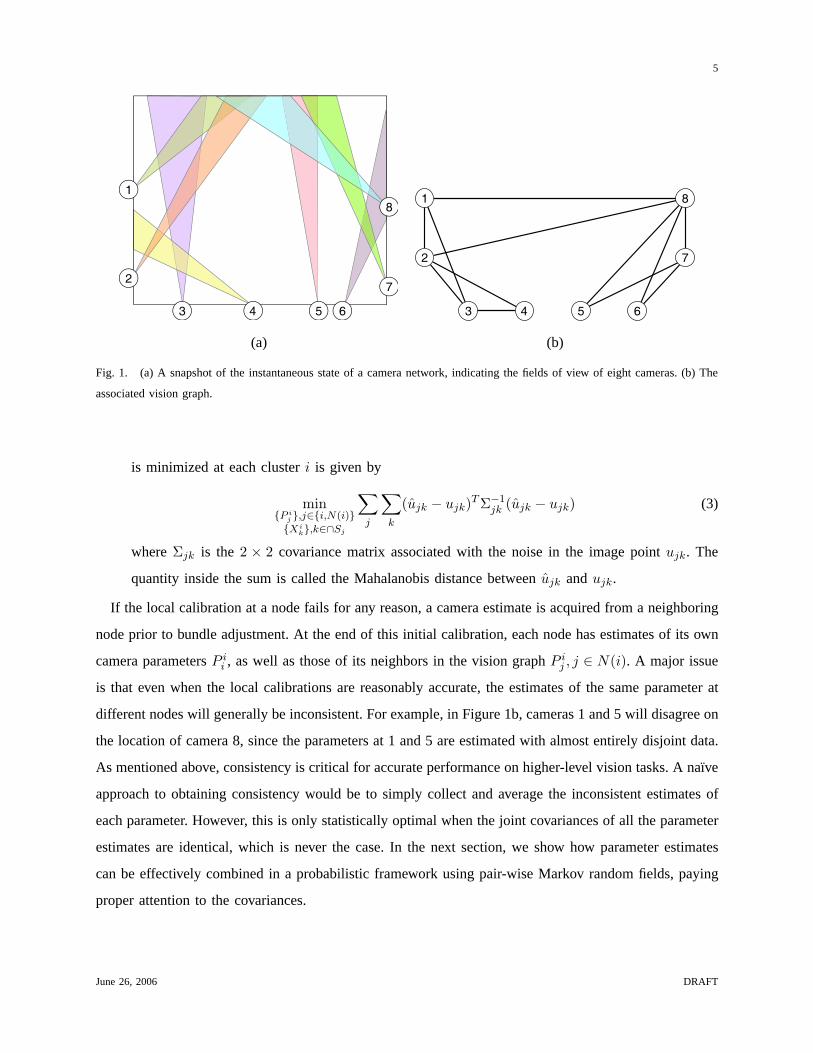
We define a graphG = (V, E) on the camera network called the vision graph, whereV is the set of

vertices (i.e. the cameras in the network) and an edge is present inE if two camera nodes observe a

sufficient number of the same scene points from different perspectives (more precisely, an edge exists if a

stable, accurate estimate of the epipolar geometry can be obtained). We define the neighbors of nodei as

N(i) = {j ∈ V |(i, j) ∈ E}. A sample camera network and its corresponding vision graph are sketched

in Figure 1.

To obtain a distributed initial estimate of the camera parameters, we use the algorithm we previously

described in [9], which roughly operates as follows at each nodei:

1) Estimate a projective reconstruction [31] based on the common scene points shared byi andN(i)

(these points are called the “nucleus”).

2) Estimate a metric reconstruction based on the projective cameras [29].

3) Triangulate scene points not in the nucleus using the calibrated cameras [2].

4) Use RANSAC [12] to reject outliers with large reprojection error, and repeat until the reprojection

error for all points is comparable to the assumed noise level in the correspondences.

5) Use the resulting structure-from-motion estimate as the starting point for full bundle adjustment

[33]. That is, if ujk represents the projection ofXik onto P i

j , then the nonlinear cost function that

June 26, 2006 DRAFT

5

1

2

3 4 5 6

7

81

2

3 4 5 6

7

8

(a) (b)

Fig. 1. (a) A snapshot of the instantaneous state of a camera network, indicating the fields of view of eight cameras. (b) The

associated vision graph.

is minimized at each clusteri is given by

min{P i

j },j∈{i,N(i)}{Xi

k},k∈∩Sj

∑

j

∑

k

(ujk − ujk)T Σ−1jk (ujk − ujk) (3)

whereΣjk is the 2 × 2 covariance matrix associated with the noise in the image pointujk. The

quantity inside the sum is called the Mahalanobis distance betweenujk andujk.

If the local calibration at a node fails for any reason, a camera estimate is acquired from a neighboring

node prior to bundle adjustment. At the end of this initial calibration, each node has estimates of its own

camera parametersP ii , as well as those of its neighbors in the vision graphP i

j , j ∈ N(i). A major issue

is that even when the local calibrations are reasonably accurate, the estimates of the same parameter at

different nodes will generally be inconsistent. For example, in Figure 1b, cameras 1 and 5 will disagree on

the location of camera 8, since the parameters at 1 and 5 are estimated with almost entirely disjoint data.

As mentioned above, consistency is critical for accurate performance on higher-level vision tasks. A naıve

approach to obtaining consistency would be to simply collect and average the inconsistent estimates of

each parameter. However, this is only statistically optimal when the joint covariances of all the parameter

estimates are identical, which is never the case. In the next section, we show how parameter estimates

can be effectively combined in a probabilistic framework using pair-wise Markov random fields, paying

proper attention to the covariances.

June 26, 2006 DRAFT

6

IV. B ELIEF PROPAGATION FORV ISION GRAPHS

Let Yi represent the true state vector at nodei that collects the parameters of that node’s camera matrix

P ii as well as those of its neighborsP i

j , j ∈ N(i), and letZi be the noisy “observation” ofYi that comes

from the local calibration process. That is, the observations arise out of local bundle adjustment on the

image projections of common scene points{ujk | j ∈ {i,N(i)}, k ∈ Si} that are used as the basis for the

initial calibration. Our goal is to estimate the true state vectorYi at each node given all the observations

by calculating the marginal

p(Yi|Z1, . . . , ZM ) =∫

{Yj ,j 6=i}p(Y1, . . . , YM |Z1, . . . , ZM ) dYj . (4)

Recently, belief propagation has proven effective for marginalizing state variables based on local

message-passing; we briefly describe the technique below. According to the Hammersley-Clifford theorem

[3], [18], a joint density is factorizable if and only if it satisfies the pair-wise Markov property,

p(Y1, Y2, ...YM ) ∝∏

i∈V

φi(Yi)∏

(i,j)∈E

ψij(Yi, Yj), (5)

where φi represents the belief (or evidence) potential at nodei, and ψij is a compatibility potential

relating each pair of nodes(i, j) ∈ E. Pearl [28] later proved that an inference on this factorized model

is equivalent to a message-passing system, where each node updates its belief by obtaining information

or messages from its neighbors. This process is what is generally referred to as belief propagation. The

marginalization is then achieved through the update equations

mtij(Yj) ∝

∫

Yi

ψ(Yi, Yj)φ(Yi)∏

k∈N(i)\jmt−1

ki (Yi) dYi (6)

bti(Yi) ∝ φ(Yi)

∏

j∈N(i)

mtji(Yi), (7)

wheremtij is the message that nodei transmits to nodej at time t, andbt

i is the belief at nodei about

its state, which is the approximation to the required marginal densityp(Yi) at time t. This algorithm is

also called the sum-product algorithm.

In our problem, the joint density in (4) can be expressed as

p (Y1, Y2, . . . YM |Z1, . . . , ZM ) ∝ p (Y1, Y2, . . . YM , Z1, . . . , ZM ) (8)

=∏

i∈V

p(Zi|Yi)∏

(i,j)∈E

p(Yi, Yj). (9)

Here,Zi is observed and hence the likelihood functionp(Zi|Yi) is a function ofYi. Similar factorizations

of the joint density are common in decoding systems [23].

June 26, 2006 DRAFT

7

p(Yi, Yj) encapsulates the constraints between the variablesYi andYj . That is, the random vectorsYi

andYj may share some random variables that must agree. We enforce this constraint by defining binary

selector matricesCij based on the vision graph as follows. LetMij be the number of variables thatYi

andYj have in common. ThenCij is a binaryMij × |Yi| matrix such thatCijYi selects these common

variables. Then we assume

P (Yi, Yj) ∝ δ(CijYi − CjiYj) (10)

whereδ(x) is 1 when all entries ofx are 0 and 0 otherwise. The joint density (10) makes the implicit

assumption of a uniform prior over the true state variables; i.e. it only enforces that common parameters

match. If available, prior information about the density of the state variables could be directly incorporated

into (10), and might result in improved performance compared to the uniform density assumption.

Therefore, we can see that (9) is in the desired form of (5), identifying

φi(Yi) ∝ p(Zi|Yi) (11)

ψij(Yi, Yj) ∝ δ(CijYi − CjiYj). (12)

Based on this factorization, it is possible to perform the belief propagation directly on vision graph

edges using the update equations (6) and (7). Figure 2 represents one step of the message passing,

indicating the actual camera parameters that are involved in each message.

1

2

3 4 5 6

7

8P

8

8P

1

8{ , }m81( )

m31( ){ , , }P

3

3P

2

3P1

3

P3

2P

2

2P

1

2({ , , })m

21

Fig. 2. An intermediate stage of message-passing.TheP ji indicate the camera parameters that are passed between nodes.

For Gaussian densities, the BP equations reduce to passing and updating the first two moments of

eachYi. Let µi represent the mean ofYi andΣi the corresponding covariance matrix. Nodei receives

estimatesµji andΣj

i from each of its neighborsj ∈ N(i). Then the update equations (6) and (7) reduce

to minimizing the sum of the KL divergences between the updated Gaussian density and each incoming

June 26, 2006 DRAFT

8

Gaussian density. Therefore, the belief update reduces to the well-known equations [30]:

µii ←

Σ−1

i +∑

j∈N(i)

(Σji )−1

−1

Σ−1i µi +

∑

j∈N(i)

(Σji )−1µj

i

(13)

Σii ←

Σ−1

i +∑

j∈N(i)

(Σji )−1

−1

. (14)

We note that (13)-(14) can be iteratively calculated in pairwise computations, instead of computed in

batch, and that this pairwise fusion is invariant to the order in which the estimates arrive.

Although (13)-(14) assume that the dimensions ofµji are the same for allj ∈ N(i), this is usually not

the case in practice, since the message sent from nodei to nodej would be a function of the subsetCijYj

rather thanYj . This can be easily dealt with by setting the entries of the mean and inverse covariance

matrix corresponding to the parameters not in the subset to 0. In this way, the dimensions of the means

and variances all agree, but the missing variables play no role in the fusion.

We obtain the mean and covariance of the assumed Gaussian densityp(Yi|Zi) based on forward

covariance propagation from bundle adjustment. That is, the covariances of the noise in the image

correspondences used for bundle adjustment are propagated through the bundle adjustment cost functional

(3) to obtain a covariance on the structure-from-motion parameters at each node [19]. Since we are

predominantly interested in localizing the camera network, we marginalize out the reconstructed 3D

structure to obtain covariances of the camera parameters alone.

V. CHALLENGES FORCAMERA CALIBRATION

The BP framework as described above is generally applicable to many information fusion applica-

tions. However, when the beliefs represent distributed estimates of camera parameters, there are several

additional difficulties, which we discuss in this section. These issues include:

1) Minimal parameterizations.Even if each camera matrix is parameterized minimally at nodei (i.e. 1

parameter for focal length, 3 parameters for camera center, 3 parameters for rotation matrix), there

are still 7 degrees of freedom corresponding to an unknown similarity transformation of all cameras

in Yi. Without modification, covariance matrices in (13)-(14) have null spaces of dimension 7 and

cannot be inverted.

2) Frame alignment.Since we assume there are no landmarks in the scene with known 3D positions,

the camera motion parameters can be estimated only up to a similarity transformation, and this

unknown similarity transformation will differ from node to node. The estimatesY ii andY j

i , j ∈ N(i)

must be brought to a common coordinate system before every fusion step.

June 26, 2006 DRAFT

9

3) Incompatible estimates.The covariances of eachYi are obtained are from independent processes,

and may produce an unreliable result in the direct implementation of (13)-(14).

We address each of the above issues in the following sections.

1) Minimal Parametrization:We minimally parameterize each camera matrixP in Yi by 7 parameters:

its focal lengthf , its camera center(x, y, z), and the axis-angle parameters(a, b, c) representing its

rotation matrix. If |{i,N(i)}| = ni, then the set of 7ni parameters is not a minimal parametrization

of the joint Yi, since the cameras can only be recovered up to a similarity transformation. Without

modification, the covariance matrices of theYi estimates will be singular.

SinceYi always includes an estimate ofPi, we apply a rigid motion so thatPi is fixed asKi[I 0]

with Ki = diag(fi, fi, 1). This eliminates 6 degrees of freedom. The remaining scale ambiguity can be

eliminated by fixing the distance between camerai and one of its neighbors (say, nodeBi); usually we

set the distance of camerai to its lowest-numbered neighbor to be 1, which means that the camera center

of Bi can be parameterized by only two spherical angles(θ, φ). We call this normalization the basis for

nodei, or Bi. Thus,Yi is minimally parameterized by a set of 7(ni-1) parameters:

Yi = [fi, fBi, θBi

, φBi, aBi

, bBi, cBi

, {fk, xk, yk, zk, ak, bk, ck, k ∈ N(i)\{i, Bi}}] (15)

The non-singular covariance ofp(Yi|Zi) in this basis can be obtained by forward covariance propagation

as described in Section IV.

2) Frame Alignment:While we have a minimal parameterization at each node, each node’s estimate

is in a different basis. In order to fuse estimates from neighboring nodes, the parameters must be in the

same frame, i.e. share the same basis cameras. In the centralized case, we could easily avoid this problem

by initially aligning all the cameras in the network to a minimally parametrized common frame (e.g. by

registering their reconstructed scene points and specifying a gauge for the structure-from-motion estimate

[22]). However, in the distributed case, it is not clear what would constitute an appropriate gauge, how it

could be estimated in a distributed manner, how each camera could efficiently be brought to the gauge,

how the gauge should change over time, and so on.

A natural approach that avoids the problem of global gauge fixing is to align the estimates ofYi to the

basisBi prior to each fusion at nodei. A subtle issue is that in this case, the resulting covariance matrices

can become singular. This is illustrated by the example in Figure 3. Consider the message to be sent from

4 to 3. The basis at 3 is formed by cameras{3,1}, and the basis at 4 is formed by cameras{4,2}. If 4

changes its basis to{3,1}, this is a reparameterization of its data from 14 to 15 parameters (i.e. initially

we have 1 parameter for camera 4, 6 for camera 2, and 7 for camera 3. After reparameterization, we

June 26, 2006 DRAFT

10

1

2

3

4

Fig. 3. Example in which the wrong method of frame alignment can introduce singularities into the covariance matrix.

would have 7 parameters for camera 4, 1 for camera 3, and 7 for camera 2), which introduces singularity

in the new covariance matrix. To avoid this problem, we use the following protocol for everyj ∈ N(i):

1) Define the basisBij as the one in whichPi = Ki[I 0] and the camera center ofPj has‖Cj‖ = 1.

2) Change both nodesi and j to basisBij .

3) Change the basis of the updated joint density atj to Bi.

We note that every basis change requires a transformation of the covariance using the Jacobian of the

transformation. While this Jacobian might have hundreds of elements (a 40×40 Jacobian is typical), it is

also sparse, and most entries can be computed analytically, except for those involving pairs of axis-angle

parameters.

3) Incompatible Estimates:The covariances that are merged at each step come from independent

processes. Towards convergence of BP, the entries of the covariance matrices become very small. When

the variances are too small (which can be detected using a threshold on the determinant of the covariance

matrix), the information matrix (i.e the inverse of the covariance matrix) has very large entries and creates

numerical difficulties in implementing (6) and (7). At this point, we make the alternate approximation that

Σji is a block diagonal matrix containing no cross-terms between cameras, with the current per-camera

covariance estimates along the diagonal. This block diagonal covariance matrix is sure to be positive

definite.

VI. EXPERIMENTS AND RESULTS

We studied the performance of the algorithm with both simulated and real data. We judge the algo-

rithm’s performance by evaluating the consistency of the estimated camera parameters throughout the

network both before and after BP. For simulated data, we also compare the accuracy of the algorithm

June 26, 2006 DRAFT

11

before and after BP with centralized bundle adjustment. On one hand, we do not expect a large change

in accuracy. The independently computed initial estimates are already reasonably good, and BP diffuses

the error from less accurate nodes throughout the network. On the other hand, we expect an increase in

the consistency of the estimates, since our main goal in applying BP is to obtain a distributed consensus

about the joint estimate.

A. Simulated Experiment

1

2

3

4

5

6

7 8 9

10

11

12

13

14

15

16

17

18

19

20

21

2223 24

25

26

27

28

29

30

(a) (b)

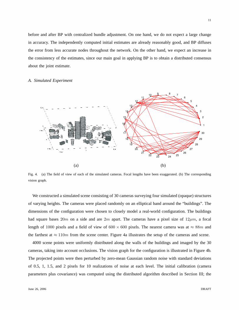
Fig. 4. (a) The field of view of each of the simulated cameras. Focal lengths have been exaggerated. (b) The corresponding

vision graph.

We constructed a simulated scene consisting of 30 cameras surveying four simulated (opaque) structures

of varying heights. The cameras were placed randomly on an elliptical band around the “buildings”. The

dimensions of the configuration were chosen to closely model a real-world configuration. The buildings

had square bases20m on a side and are2m apart. The cameras have a pixel size of12µm, a focal

length of 1000 pixels and a field of view of600 × 600 pixels. The nearest camera was at≈ 88m and

the farthest at≈ 110m from the scene center. Figure 4a illustrates the setup of the cameras and scene.

4000 scene points were uniformly distributed along the walls of the buildings and imaged by the 30

cameras, taking into account occlusions. The vision graph for the configuration is illustrated in Figure 4b.

The projected points were then perturbed by zero-mean Gaussian random noise with standard deviations

of 0.5, 1, 1.5, and 2 pixels for 10 realizations of noise at each level. The initial calibration (camera

parameters plus covariance) was computed using the distributed algorithm described in Section III; the

June 26, 2006 DRAFT

12

Noise level Cerr

σ (pixels)Network State

(cm)θerr ferr

Initialization 14.2 1.3e-3 0.0035

0.5 Convergence 13.9 1.5e-3 0.0029

Centralized Bundle 12.3 0.9e-3 0.0015

Initialization 24.2 2.5e-3 0.0064

1 Convergence 22.9 2.3e-3 0.0051

Centralized Bundle 24.3 1.7e-3 0.0031

Initialization 43.3 4.2e-3 0.0129

1.5 Convergence 44.2 4.0e-3 0.0081

Centralized Bundle 41.8 2.8e-3 0.0052

Initialization 48.5 5.5e-3 0.0144

2 Convergence 55.7 4.5e-3 0.0115

Centralized Bundle 43.6 4.2e-3 0.0064

TABLE I

SUMMARY OF THE CALIBRATION ACCURACY. Cerr IS THE AVERAGE ABSOLUTE ERROR IN CAMERA CENTERS IN CM

(RELATIVE TO A SCENE WIDTH OF220M). θerr IS THE AVERAGE ORIENTATION ERROR BETWEEN ROTATION MATRICES

GIVEN BY (18).ferr IS THE AVERAGE FOCAL LENGTH ERROR AS A RELATIVE FRACTION.

correspondences and vision graph are assumed known (since there are no actual images in which to

detect correspondences). Belief propagation was then performed on the initialized network as described

in Sections IV and V. The algorithm converges when there are no further changes in the beliefs; in our

experiments we used the convergence criterion‖Y ti − Y t−1

i ‖/‖Y t−1i ‖ < 0.001. In our experiments, the

number of BP iterations ranged from 4 to 12.

The accuracy of the estimated parameters, both before and after BP, is reported in Table I. We

first aligned each node to the known ground truth by estimating a similarity transformation based

on corresponding camera matrices. The error metrics for focal lengths, camera centers, and camera

June 26, 2006 DRAFT

13

orientations are computed as:

d(f1, f2) = |1− f1/f2| (16)

d(C1, C2) = ‖C1 − C2‖ (17)

d(R1, R2) = 2√

1− cos θ12 (18)

whereθ12 is the relative angle of rotation between rotation matricesR1 andR2. Table I reports the mean

of each statistic over the 10 random realizations of noise at each level. As Table I shows, there is little

change in the relative accuracy of the network calibration before and after BP (in fact, the accuracy of

camera centers and orientations is slightly worse after BP in noisy cases, and the accuracy of focal lengths

slightly better). However, the accuracy is quite comparable with that of centralized bundle adjustment

with a worst case camera center error of 56cm vs 44cm for the 2 pixel noise level (recall the scene is

220m wide).

The consistencyof the estimated parameters, both before and after BP, is reported in Table II. For

each nodei, we aligned each neighborj ∈ N(i) to basisBi, and scaled the dimensions of the result

to agree with ground truth. We then measured the consistency of all estimates off ji , Cj

i , and Rji by

computing the standard deviation of each metric (16)-(18), usingf ii , C

ii , R

ii as a reference. The mean of

the deviations for each type of parameter over all the nodes was computed, and averaged over the 10

random realizations of noise at each level.

As Table II shows, the inconsistency of the camera parameters before and after BP is reduced by

factors of approximately 2 to 4, with increasing improvement at higher noise levels. Higher-level vision

and sensor networking algorithms can definitely benefit from the accurate, consistent localization of the

nodes, which was obtained in a completely distributed framework.

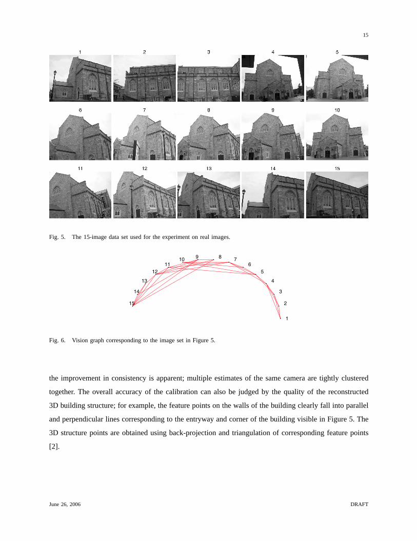
B. Real Experiment

We also approximated a camera network using 15 real images of a building captured by a single

camera from different locations (Figure 5). The corresponding vision graph is shown in Figure 6 and was

obtained by the automatic algorithm also described in this special issue [4]. The images were taken with

a Canon G5 digital camera in autofocus mode (so that the focal length for each camera is different and

unknown). A calibration grid was used beforehand to verify that for this camera, the skew was negligible,

the principal point was at the center of the image plane, the pixels were square, and there was virtually

no lens distortion. Hence the assumed pinhole projection model with a diagonalK matrix is justified in

this case.

June 26, 2006 DRAFT

14

Noise level Csd

σ (pixels)Network State

(cm)θsd fsd

Initialization 20.9 1.6e-3 0.0029

0.5 Convergence 11.3 9.8e-3 0.0016

Improvement factor 1.9 1.7 1.8

Initialization 31.7 2.9e-3 0.0025

1 Convergence 11.8 1.2e-3 0.0011

Improvement factor 2.7 2.4 2.7

Initialization 58.4 4.6-3 0.0056

1.5 Convergence 16.8 2.1e-3 0.0018

Improvement factor 3.5 2.2 3.1

Initialization 63.4 6.2e-3 0.0079

2 Convergence 15.5 1.6e-3 0.0021

Improvement factor 4.1 3.8 3.8

TABLE II

SUMMARY OF THE CALIBRATION CONSISTENCY. Csd IS THE AVERAGE STANDARD DEVIATION OF ERROR IN CAMERA

CENTERS IN CM(RELATIVE TO A SCENE WIDTH OF220M). θsd IS THE AVERAGE STANDARD DEVIATION OF ORIENTATION

ERROR BETWEEN ROTATION MATRICES GIVEN BY(18).fsd IS THE AVERAGE STANDARD DEVIATION OF FOCAL LENGTH

ERROR.

As in the previous experiment, we obtained the distributed initial calibration estimate using the proce-

dure described in Section III. We analyzed the performance of the algorithm by measuring the consistency

of the camera parameters before and after belief propagation. Table III summarizes the result. Since the

ground truth dimensions of the scene are unknown, the units of the camera center standard deviation are

arbitrary. The performance is best judged by the improvement factor, which is quite significant for the

camera centers (a factor of almost 6), which would be important for good performance on higher-level

vision and sensor networking algorithms in the real network.

Figure 7 shows the multiple estimates of a subset of the cameras (aligned to the same coordinate frame)

both before and after the belief propagation algorithm. Before belief propagation, the estimates of each

camera’s position are somewhat spread out and there are several outliers (e.g. one estimate of camera

13 is far from the other two, and very close to the corner of the building). After belief propagation,

June 26, 2006 DRAFT

15

Fig. 5. The 15-image data set used for the experiment on real images.

1

2

3

4

5

6

7 8 9

10

11

12

13

14

15

Fig. 6. Vision graph corresponding to the image set in Figure 5.

the improvement in consistency is apparent; multiple estimates of the same camera are tightly clustered

together. The overall accuracy of the calibration can also be judged by the quality of the reconstructed

3D building structure; for example, the feature points on the walls of the building clearly fall into parallel

and perpendicular lines corresponding to the entryway and corner of the building visible in Figure 5. The

3D structure points are obtained using back-projection and triangulation of corresponding feature points

[2].

June 26, 2006 DRAFT

16

Network State Csd θsd fsd (pixels)

Initialization 0.1062 0.7692 126.81

Convergence 0.0184 0.3845 84.22

Improvement factor 5.77 2 1.5

TABLE III

SUMMARY OF THE CALIBRATION CONSISTENCY. Csd IS THE AVERAGE STANDARD DEVIATION OF ERROR IN CAMERA

CENTERS(IN ARBITRARY UNITS). θsd IS THE AVERAGE STANDARD DEVIATION OF ORIENTATION ERROR BETWEEN

ROTATION MATRICES GIVEN BY (18).fsd IS THE AVERAGE STANDARD DEVIATION OF ABSOLUTE FOCAL LENGTH ERROR IN

PIXELS.

1

1

1

2

2

2

8

3

3

3

10

13

13

Entryway

Sidewall

1

2

3

8

10

13

Entryway

Sidewall

Fig. 7. Multiple camera estimates of a subset of cameras (a) before and (b) after belief propagation. The numbers correspond

to the node numbers in Figures 5 and 6.

VII. C ONCLUSIONS

We demonstrated the viability of using belief propagation to obtain the accurate, consistent calibration

of a camera network in a fully distributed framework. We took into consideration several unique practical

aspects of working with sets of camera parameters, such as overdetermined parameterizations, frame

alignment, and inconsistent estimates. Our algorithm is distributed, with computations based only on

June 26, 2006 DRAFT

17

local interactions, and hence is scalable. The improvement in consistency is achieved with only a small

loss of accuracy. In comparison, a centralized bundle adjustment would involve an optimization over a

huge number of parameters and would pose challenges for scalability of the algorithm.

The framework proposed here could also incorporate other recently proposed algorithms for robust

distributed inference, as described in Section II. While the forms of the passed messages might change,

we believe that our insights into the fundamental challenges of dealing with camera networks would

remain useful. Improved inference schemes might also have the benefit of allowing asynchronous updates

(since BP as we described it here is implicitly synchronous).

In the future, we plan to investigate higher-level distributed vision applications on camera networks,

such as shape reconstruction and object tracking, that further demonstrate the importance of using con-

sistently localized cameras. Finally, we plan to analyze networking aspects of our algorithm (e.g. effects

of channel noise or node failures) that would be important in a real deployment.

REFERENCES

[1] M. Alanyali, S. Venkatesh, O. Savas, and S. Aeron. Distributed Bayesian hypothesis in sensor networks. InProceedings

of the American Control Conference, June 2004.

[2] M. Andersson and D. Betsis. Point reconstruction from noisy images.Journal of Mathematical Imaging and Vision,

5:77–90, January 1995.

[3] J. Besag. Spatial interaction and the statistical analysis of lattice systems.Journal of the Royal Statistical Society,

B(36):192–236, 1974.

[4] Z. Cheng, D. Devarajan, and R. Radke. Determining vision graphs for distributed camera networks using feature digests.

EURASIP Journal of Applied Signal Processing, Special Issue on Visual Sensor Networks, 2006.

[5] C. Christopher and P. Avi. Loopy belief propagation as a basis for communication in sensor networks. InProceedings of

the 19th Annual Conference on Uncertainty in Artificial Intelligence (UAI-03), pages 159–166, San Francisco, CA, 2003.

Morgan Kaufmann Publishers.

[6] J. M. Coughlan and S. J. Ferreira. Finding deformable shapes using loopy belief propagation. InProceedings of the 7th

European Conference on Computer Vision (ECCV ’02), pages 453–468, London, UK, 2002. Springer-Verlag.

[7] L. Davis, E. Borovikov, R. Cutler, D. Harwood, and T. Horprasert. Multi-perspective analysis of human action. In

Proceedings of the 3rd International Workshop on Cooperative Distributed Vision, November 1999. Kyoto, Japan.

[8] F. Dellaert, A. Kipp, and P. Krauthausen. A multifrontal QR factorization approach to distributed inference applied to

multirobot localization and mapping. InProceedings of National Conference on Artificial Intelligence (AAAI 05), pages

1261–1266, 2005.

[9] D. Devarajan, R. J. Radke, and H. Chung. Distributed metric calibration of ad-hoc camera networks.ACM Transactions

on Sensor Networks, 2006. Accepted, to appear.

[10] H. F. Durrant-Whyte and M. Stevens. Data fusion in decentralized sensing networks. InProceedings of the 4th International

Conference on Information Fusion, 2001.

[11] P. F. Felzenszwalb and D. P. Huttenlocher. Efficient belief propagation for early vision. InProceedings of IEEE Conference

on Computer Vision and Pattern Recognition, pages 261–268, 2004.

June 26, 2006 DRAFT

18

[12] M. A. Fischler and R. C. Bolles. Random sample consensus: A paradigm for model fitting with applications to image

analysis and automated cartography.Communications of the ACM, 24:381–395, 1981.

[13] W. Freeman, E. Pasztor, and O. Carmichael. Learning low-level vision.International Journal of Computer Vision, 40(1):25–

47, 2000.

[14] W. T. Freeman and E. C. Pasztor. Learning to estimate scenes from images. In M. S. Kearns, S. A. Solla, and D. A. Cohn,

editors,Advances in Neural Information Processing Systems 11. MIT Press, 1999.

[15] B. J. Frey.Graphical Models for Pattern Classification, Data Compression and Channel Coding. MIT Press, 1998.

[16] S. Funiak, C. Guestrin, M. Paskin, and R. Sukthankar. Distributed localization of networked cameras. InInternational

conference on Information processing in Sensor Networks (IPSN-06), Nashville, TN, USA, April 2006.

[17] S. Grime and H. F. Durrant-Whyte. Communication in decentralized systems.IFAC Control Engineering Practice,

2(5):849–863, 1994.

[18] J. Hammersley and P. E. Clifford. Markov fields on finite graphs and lattices. Unpublished article, 1971.

[19] R. Hartley and A. Zisserman.Multiple View Geometry in Computer Vision. Cambridge University Press, 2000.

[20] M. Isard and A. Blake. Condensation – conditional density propagation for visual tracking.International Journal of

Computer Vision, 29(1):5–28, 1998.

[21] T. Kanade, P. Rander, and P. Narayanan. Virtualized reality: Constructing virtual worlds from real scenes.IEEE Multimedia,

Immersive Telepresence, 4(1):34–47, January 1997.

[22] K. Kanatani and D. D. Morris. Gauges and gauge transformations for uncertainty description of geometric structure with

indeterminacy.IEEE Transactions on Information Theory, 47(5):2017–2028, July 2001.

[23] F. Kschischang, B. J. Frey, and H.-A. Loeliger. Factor graphs and the sum-product algorithm.IEEE Transactions on

Information Theory, 47, 2001.

[24] R. McEliece, D. MacKay, and J.-F. Cheng. Turbo decoding as an instance of Pearl’s “belief propagation” algorithm.IEEE

Journal on Selected Areas in Communications, 16(2):140–152, February 1998.

[25] K. P. Murphy, Y. Weiss, and M. I. Jordan. Loopy belief propagation for approximate inference: An empirical study. In

Proceedings of Uncertainty in Artificial Intelligence (UAI ’99), pages 467–475, 1999.

[26] M. A. Paskin and C. E. Guestrin. Robust probabilistic inference in distributed systems. InProceedings of the twentieth

Conference on Uncertainty in Artificial Intelligence (UAI ’04), pages 436–445, Arlington, VA, USA, 2004. AUAI Press.

[27] M. A. Paskin, C. E. Guestrin, and J. McFadden. A robust architecture for inference in sensor networks. In4th International

Symposium on Information Processing in Sensor Networks (IPSN ’05), 2005.

[28] J. Pearl.Probablistic Reasoning in Intelligent Systems. Morgan Kaufmann, 1988.

[29] M. Pollefeys, R. Koch, and L. J. Van Gool. Self-calibration and metric reconstruction in spite of varying and unknown

internal camera parameters. InProceedings of the 6th IEEE International Conference on Computer Vision (ICCV ’98),

pages 90–95, 1998.

[30] R. Smith, M. Self, and P. Cheeseman. Estimating uncertain spatial relationships in robotics. InAutonomous Robot Vehicles,

pages 167–193. Springer-Verlag New York, Inc., New York, NY, USA, 1990.

[31] P. Sturm and B. Triggs. A factorization based algorithm for multi-image projective structure and motion. InProceedings

of the 4th European Conference on Computer Vision (ECCV ’96), pages 709–720, 1996.

[32] E. B. Sudderth, M. I. Mandel, W. T. Freeman, and A. S. Willsky. Distributed occlusion reasoning for tracking with

nonparametric belief propagation. In L. K. Saul, Y. Weiss, and L. Bottou, editors,Advances in Neural Information

Processing Systems 17, pages 1369–1376. MIT Press, Cambridge, MA, 2005.

[33] B. Triggs, P. McLauchlan, R. Hartley, and A. Fitzgibbon. Bundle adjustment – A modern synthesis. In W. Triggs,

June 26, 2006 DRAFT

19

A. Zisserman, and R. Szeliski, editors,Vision Algorithms: Theory and Practice, LNCS, pages 298–375. Springer Verlag,

2000.

[34] Y. Weiss and W. T. Freeman. Correctness of belief propagation in Gaussian graphical models of arbitrary topology.

Advances in Neural Information Processing Systems (NIPS), 12, November 1999.

[35] J. S. Yedidia, W. Freeman, and Y. Weiss. Understanding belief propagation and its generalizations. In G. Lakemeyer and

B. Nebel, editors,Exploring Artificial Intelligence in the New Millennium, chapter 8, pages 239–236. Morgan Kaufmann,

2003.

June 26, 2006 DRAFT